Metallicity gradients in the Sagittarius dwarf spheroidal Galaxy.

Metallicity gradients in the Sagittarius dwarf Galaxy (Sgr) are investigated by using infrared photometric data from the 2MASS survey. To search for metallicity effects, the giant branch in a field situated near the Center of the Sgr is compared to the giant branch in a field situated near its southern edge. The contamination of Sgr giant branch by foreground Galactic stars is canceled by statistical subtraction of diagrams symmetrical in Galactic latitude. After subtraction it is possible to reconstruct the Sgr giant branch with excellent accuracy. The giant branch in the two fields have similar slopes but are shifted in color. Even after correction for the differential reddening between the fields, the shift in color between the branch remains, and is very significant. This variation in the color of the giant branch corresponds to a metallicity variation of about -0.25 Dex. The existence of a metallicity gradient in Sgr may indicate that there are two different stellar population in Sgr. One has low metallicity, and another one of higher metallicity has a smaller spatial extension.

1 Introduction

The closest and largest Galaxy on the sky, the Sagittarius dwarf galaxy (Sgr) has been discovered only recently (Ibata, Gilmore, & Irwin 1994 (IGI)). This Galaxy seems to be a dwarf spheroidal situated only 25 Kpc from us and only 16 Kpc from the Galactic center . Most of Sgr is situated at low Galactic latitudes and is seen through a dense screen of stars from the Milky Way. Even at the center of Sgr (b $\simeq$ -14), the density on sky of stars from the Milky way is overwhelming. This situation explains why the detection of Sgr is so difficult, and could be achieved only recently. One possible way to separate stars from Sgr and the Galaxy is to measure the radial velocity. There is a systematic difference of about 200 kms^-1 for stars in Sgr and stars in the Milky way. This large difference of velocity permitted the discovery of Sgr by IGI. Another method to identify stars in Sgr is to search for RR Lyrae variables. The RR Lyrae stars are good standard candles, and they can be used to probed the distribution of the stellar density as a function of distance. The histogram of the RR Lyrae magnitude of a field in Sgr shows a double peaked distribution. The first peak corresponds to the Galaxy, while the second peak corresponds to Sgr (Alard 1995). By selecting RR Lyrae in the second peak it is possible to map the spatial distribution of Sgr. Using this method it was possible to identify a new extension of Sgr at lower Galactic latitudes (Alard 1996). This work was recently extended in order to produce a large map of Sgr, from the lower latitude extension to the center of the Galaxy (Alard, Cseresnjes,& Guibert 2000). In addition to the radial velocities and the RR Lyrae, there are photometric methods that can be used to probe the structure of Sgr. For instance, IGI used a feature in a $B_{J}$ vs. $B_{J}$-R color magnitude diagram to identify stars in Sgr. However the method is not very efficient at lower Galactic latitude, due to contamination by the Galaxy. Using similar color magnitude diagrams, Bellazzini, Ferraro, & Buonanno (1999) were able to further the study of Sgr stellar populations. They demonstrate that a very metal-poor population is present in Sgr, and they show possible hints for a metallicity gradient in Sgr. The advent of new infrared data from the 2MASS survey offers is very promising for the study of Galactic structure in general. There are well-defined structures in the infrared color magnitude diagrams, like the upper giant branch, which can be very useful to probe the structure of Galaxies. Furthermore, the dramatic weakening of the interstellar extinction obtained by going to the infrared is a very important asset. We will see that these infrared color magnitude diagrams are a efficient tool used to study the stellar population of Sgr.

2 The Data

Two fields have been selected to investigate the metallicity effects in Sgr. One of the fields is close to the center of the Galaxy, while the other is close the lower latitude edge of the Galaxy according to the map of Ibata et al. (1995) (see Fig. 1). All the stellar magnitudes have been extracted from the 2MASS point source catalogue. The stellar populations in these fields are well characterized by their K vs. (J-K) color magnitude diagrams . To identify features or sequences which are not related to the Galactic population, it is interesting to compare these diagrams with diagrams obtained from fields symmetrical in Galactic coordinates (see table 1 for a summary of the fields location). By comparing the symmetrical diagrams we see immediately that for the fields in Sgr, an additional sequence is present at the right of the diagrams (see Fig 2). This sequence is visible for the field at the center of Sgr, but also for the field near the lower latitude edge. This feature is certainly associated with the upper giant branch of Sgr. The tip of the sequence is approximately at K$=$10.5 which is consistent with an object at a distance of 25 Kpc.

Table 1: The fields

Field	field center	size of field
Center	(l,b)$=$(6,-14)	($\Delta$l,$\Delta$b)$=$(2,2)
Edge	(l,b)$=$(6.5,-20)	($\Delta$l,$\Delta$b)$=$(2,2)
Center-sym	(l,b)$=$(6,14)	($\Delta$l,$\Delta$b)$=$(2,2)
Edge-sym	(l,b)$=$(6.5,20)	($\Delta$l,$\Delta$b)$=$(2,2)

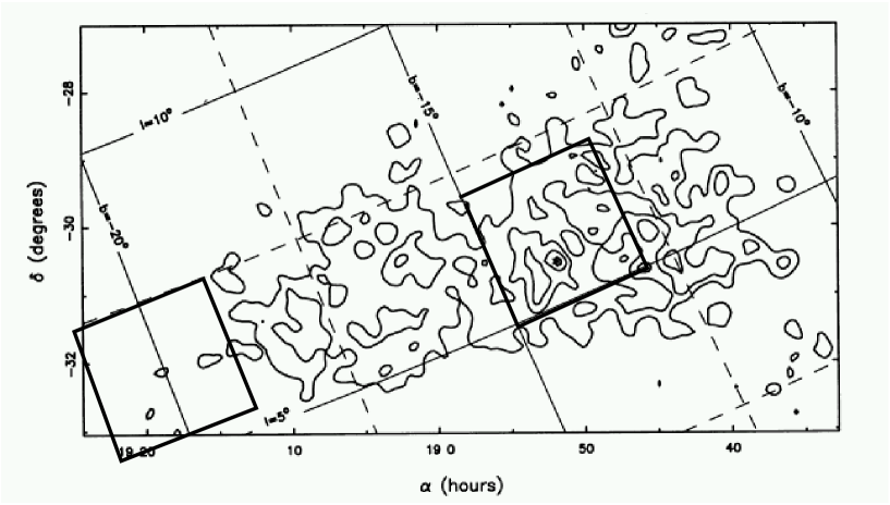
Figure 1: The position of the 2 fields in Sgr, superimposed on the map of Ibata et al. (1995)

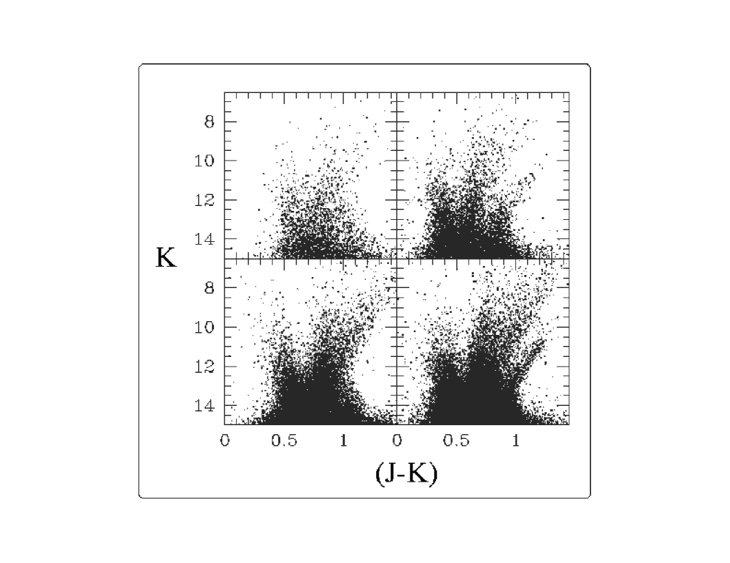
Figure 2: The K vs. (J-K) color magnitude diagrams for the 4 fields. The fields in Sgr are on the right side of the diagram, while the field at the symmetrical position in Galactic coordinates are to the left. The upper right diagram is for the field near the edge of Sgr, and the lower right diagram for a field at the center of Sgr.

3 Reconstruction of Sgr giant branch

The Sgr giant branch is nicely visible in the color magnitude diagrams of our two fields. In general, the contamination of the Sgr giant branch by stars from the Galaxy is a serious problem. However, for bright stars (K$>$12) there is very little contamination of the Sgr giant branch by foreground Galactic stars. Thus it is possible to use this bright tip of the giant branch to estimate its width. Before looking at the width of the branch, it is interesting to apply a small rotation to the diagram in order to have the branch vertical. This can be achieved easily by defining the new color index: $(J-K)_{E}=(J-K)-\frac{K-11}{50}$ .  By making an histogram using the modified color index $(J-K)_{E}$ for stars brighter than (K$=$12), and by fitting a gaussian around the position of the branch, we can estimate the width of the branch. The results of the fitting are summarized in Table 2. There is no significant difference in the width of the branch between the two fields. This width is somewhat larger than the internal scatter, as derived from the errors on measuring the magnitudes, quoted in this release of the 2MASS catalogue. It shows that the mean scatter in metallicity in Sgr is probably quite small.

Table 2: The two fields

Field	Position of the branch	Width
Sgr center	$(J-K)_{E}=1.07$	$\sigma=0.0484$
Sgr edge	$(J-K)_{E}=0.99$	$\sigma=0.0498$

To proceed further in our analysis, we need to estimate the slope and the position of the giant branch in the two fields. It is not possible to restrict our analysis to the brighter stars to estimate the shape of the branch. The dynamical range would not be sufficient. Thus we need to extend our fitting procedure to the fainter stars which are contaminated by the Galactic foreground stars. A simple solution to this contamination problem is to subtract the contribution from the Galaxy by assuming that the Galaxy is symmetrical in latitude.

3.1 Subtraction of the diagrams.

In practice, the subtraction can be performed by binning the data. We use the same bin size for all the data in K; the size of the bin is 0.1 mag. and is 0.025 mag in (J-K). Before we can subtract the diagram we have to compensate for the differential reddening between the fields. This differential reddening can be estimated by searching for the maximum correlation between parts of the diagrams which are far from the giant branch. The area we selected for cross correlation is presented in Fig. 3. Once the reddening alignment has been performed, we subtract the diagrams, and normalize the residuals by the square root of variance of the noise in the subtracted image. The noise is estimated in the region of the diagram that we already used to estimate the differential reddening. As we expect from Poisson statistics, the variance of the noise is correlated to the counts in the initials diagrams. However the statistics of the residual is larger than the Poissonian expectation the reason for this is probably that the reddening variation as a function of distance is nor perfectly identical between symmetrical Galactic fields. Another possibility is that the distribution of stars in the Galaxy is not perfectly symmetrical. It is possible that the Galactic bar is slightly tilted out of the plane, or that the structure of the spiral arms are not perfectly smooth. These small asymmetries are sufficient to create an additional source of noise in the diagrams. However, it is important to note that these additional fluctuations are unlikely to create significant systematic biases. First, there are no reason that the (small) effect of extinction be correlated between the two fields. Secondly, even if some asymmetries exist in the Galaxy between positive and negative longitude, the effect cannot be large (the amplitude of a spiral arms is only 5 to 10 % of the density). Even in the low density regions near the edge of Sgr, the density of Sgr giant branch in the CMD diagram is comparable to the density of Galactic stars, thus the systematic effects should stay beyond 10 %, which is not much larger than the basic statistical fluctuations (Poisson noise). Finally, the subtracted diagrams normalized by the noise expectation are smoothed using a 3$\times$3 mesh. The two diagrams we obtain are presented in Fig. 4.

3.2 Location of the giant branch.

Once the diagrams have been decontaminated by the subtraction process, we can measure with good accuracy the position of the Sgr giant branch. Since the branch is almost vertical, its location can be found by estimating the position of its intersection with a horizontal line. In the K vs. (J-K) plane this is almost equivalent to searching for the maximum of the histogram in (J-K) of a strip defined by the condition: $K_{0}<K<K_{0}+\Delta K$. This histogram corresponds to a line in the image of the cmd presented in Fig. 4 (reconstructed by binning the cmd). An estimate of the giant branch position is given by the position of the pixel with maximum counts. Let us call $nx_{1}$ the value of the pixel at maximum, and $x_{1}$ the position of this pixel (integer number). This position has an accuracy which is not better than the pixel size. It is possible to improve the accuracy by using the neighboring pixels, with positions ($x_{0}=x1-1$, $x_{2}=x1+1$), and associated pixel values ($nx_{1}$, $nx_{2}$). To refine the position, we will use a parabolic interpolation. Then the location of the maximum can be calculated by adding a fraction of a pixel shift given by the formula: $\delta_{X}=0.5\frac{(nx_{0}-nx_{2})}{nx_{2}+nx_{0}-2\ nx_{1}}$. The position of the giant branch in the two field has been reconstructed using this method (Fig. 5). The slope of giant branch in the two fields is not significantly different. However, it is clear that the giant branch corresponding to the field near the edge of Sgr is redder than at the center of Sgr. However, before we can claim any difference in the color of the giant branch between these two fields, we have to compensate for the differential reddening between the center and the edge of Sgr.

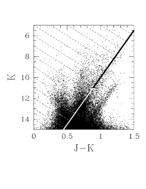
Figure 3: Color magnitude diagram of the field near the center of Sgr. The area of the diagram we used to estimate the differential reddening between the fields is indicated by dashed lines.

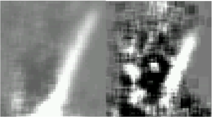
Figure 4: The subtracted images obtained by using the procedure described in Spec. 3.1. Left is the subtracted image corresponding to the field near the center of Sgr. The other image corresponds to the field near the edge of Sgr, near b$=$-20.

Figure 5: Reconstruction of the giant branch in the two fields. The location of the giant branch as been estimated by using the subtracted diagrams presented in Fig. 4.

3.3 Differential reddening between the 2 fields in Sgr.

To estimate the differential reddening between the field at the center of Sgr and the field near the edge, we will use the stars situated in the upper left region of the color magnitude diagram. The upper left region will be defined by the following conditions: (J-K)-(K-11)$/50<0.8$ and K$<12$.  The upper left region of the color magnitude diagrams is occupied by main sequence stars located in foreground regions of the Galactic disk. These stars are relatively close (a few Kpc), but at latitude $b>14^{\circ}$ the line of sight escapes very quickly the thin layer where the interstellar material is concentrated. Thus it is very unlikely that reddening occur beyond a few Kpc from the sun for our two fields, and consequently, the differential reddening of Sgr can be estimated by using foreground disk stars situated a few Kpc from us. One may also wonder metallicity gradients in the disk effects can bias our differential estimation of the reddening. However, between the field near Sgr center and the field at the edge of Sgr, the difference in height above the plane is less than 0.1 Kpc. It is unlikely that such small difference in height above the plane will result in a systematic difference in color (due to metallicity effects) between the two lines of sight. A metallicity gradient in Sgr cannot be mimicked by a metallicity gradient in the Galaxy. The effects have opposite directions. Even if a small difference in metallicity existed, it would result only in a slight under-estimation of the metallicity gradient between the two fields in Sgr. The differential reddening is estimated by cross correlation between the sequences of foreground stars in the two fields. The cross correlation is estimated after binning the data along the color axis. The color has been slightly modified to take into account the slope of the sequence using our former relation (Color$=$(J-K)-(K-11)$/50<0.8$). The maximum correlation as a function of the differential reddening between the fields is estimated by fitting a parabola to the data (see Fig. 6). The estimated differential reddening between the fields is 0.031 mag with an error close to 0.0015 mag. Considering that the uncorrected difference in color between the two giant branches is 0.075 mag, the reddening$-$corrected difference in color is 0.044 mag. The total error on this differential color is only about 0.006 mag. There is no doubt that we have found a very significant color effect in Sgr. However, before claiming a systematic color difference between the two giant branches, one may wonder if this shift cannot be interpreted as a differential distance effect between the two fields. A color shift of 0.044 mag in (J-K) corresponds to a shift in K of about $0.044\times$ (GB Slope) $\simeq$ 0.45 mag. At the distance of Sgr it corresponds to a difference in distance of about 5 Kpc. However, the projected distance between the field is only of $\simeq$ 2.5 Kpc. The projected distance is an upper limit, in reality, due to the extension of the Sgr body, even if Sgr is highly inclined, the mean effect will be smaller. Thus this shift in color cannot be interpreted as an effect of distance. Note also that this systematic shift is statistical. This is a mean difference between a large number of stars. Thus even if some spread in distance exists between individual stars due to the extent of Sgr along the line of sight (as illustrated by Bonifacio el al. 2000, Ibata et al. 1997, and Helmi & White(2001)), what we measure, which is the mean location of the giant$-$branch is well defined statistically. The internal scatter in distances within Sgr will result in some broadening of the giant branch. According to the result given in Table 2, an internal scatter of a few Kpc within Sgr body is possible, but it is very hard to be more specific, since we are limited by the photometric errors.

Figure 6: Cross correlation between the sequence of foreground stars for the two fields in Sgr. The cross correlation is plotted as a function of the differential reddening between the field near the edge and the field near the center of Sgr.

4 Measuring the metallicity gradient in Sgr.

We detected a significant shift in the color of the giant branch between the center and edge of Sgr. This shift can be due either to a systematic variation in age or metallicity of the stellar population in Sgr. One may interpret this color shift as a metallicity variation . The metallicity inferred from the slope of the giant branch using the Kuchinski & Frogel (1995) relation are: $[Fe/H]=-2.98-23.84{\rm\times(GB\ Slope)}=-0.37\pm 0.04$ near Sgr center, and $[Fe/H]=-0.41\pm 0.1$ at the edge of Sgr (note the errors quoted here are internal errors). First, we note that the metallicity inferred using the Kuchinski relation for Sgr giants is not far from the metallicity measured by Bonifacio for two giants in Sgr ( $[Fe/H]=-0.28$ and $[Fe/H]=-0.21$ ). This metallicity estimation is also consistent with the metallicity calculated by Dudziak et al. (2000) who found $[Fe/H]=-0.55$ Some other studies seems to reveal a mixture of populations in Sgr. For instance, Smecker-hane, Mc William & Ibata (1998) analyzed the spectra of 7 stars in Sgr. Some of the stars show solar metallicity abudances, while some have metallicity comparable to stars in the Galactic Halo. Bellazzini, Ferraro, & Buanono (1999) found similar results by analyzing V, (V$-$I) color magnitude diagrams in Sgr. Finally, a metal poor population was identified in M54 (Brown, Wallerstein, & Gonzalez 1999). Thus, measuring a metallicity in Sgr may depend on the type of the stellar population under investigation. The result we obtained indicates that our sample of giants belongs to the metal rich population in Sgr, but obviously we do not detect any significant metallicity variations between the two fields by this method. However, in Sec. 3.3 we found a very significant difference in the color of the branch in the two fields. According to the linear relation presented in Fig. 8, this color shift corresponds to about 0.2 Dex in metallicity. This result is consistent (within the uncertainties in measuring the slope) with our previous measurements of the metallicity using the Kuchinski & Frogel (1995) relation. We can conclude that mean metallicity of our Sgr giants seems to be about -0.4 Dex, with a systematic trend of about 0.2 Dex from the center to the edge of the Galaxy. Concerning internal metallicity dispersion within each field, we remind the reader that the width of the giant branch is about 0.05 mag in the (J-K) color index (Sec. 3). According to the linear relation presented in Fig. 8, this width corresponds to about 0.25 Dex in metallicity. We may conclude that the internal dispersion in metallicity is about 0.25 Dex. However, it is possible that a small fraction of the total number of stars has a much lower metallicity that the mean. Such a small tail in the metallicity distribution is very hard to identify using color magnitude diagrams.

5 Discussion

We may also interpret our results as a possible age variation. However, the effect of age on color is weak. For instance, at a metallicity close to -0.4 Dex, using the theoretical isochrones of Bertelli et al. 1994, & Girardi et al. 1996 we find that the maximum difference in color obtained for 17.4 Gyr and 6.8 Gyr is 0.056 mag in (J-K) (see Fig. 7). Thus, it is possible that age has an effect on the observed color shift, but this effect is probably not dominant. Thus we can conclude that the stellar population in Sgr is slightly older and slightly more metal poor near the edge of Sgr than at its center, with a metallicity effect close to 0.2 Dex. It is important to notice that similar metallicity gradients have been found in other dSph. Da Costa et al. 1996 showed by analyzing HST color$-$magnitude data from satellites of M31 that the morphology of the horizontal branch (HB) differs from the center to the outer parts for 2 out of 3 of the dSph’s in the sample. This change in the HB morphology suggests the possibility of a metallicity gradient. Similarly, Hurley$-$Keller, Mateo & Grebel (1999) describe a change in the HB morphology in their study of the Sculptor dwarf galaxy. One may interpret the metallicity gradient in Sgr as a smooth variation of the chemical composition of a single stellar population in Sgr. This might be more easily represented if we assume that Sgr is composed of two different stellar populations. These two populations could be a metal$-$poor component (Halo), and a more metal$-$rich component with less spatial extension. The combination of both population is such that the Halo becomes dominant only near the edge. One may wonder what the more metal rich component could be. If we compare this Galaxy to a dwarf Galaxy with similar metallicity (The LMC) we find that this more metal$-$rich component may look like a disk. Since disks are fragile to dynamical perturbations, in the case of Sgr we would observe only the remains of a tidally disrupted disk. This scenario is consistent with the dynamical simulations recently performed by Mayer et al. 2001 which show that small irregular galaxies constituted of a disk and a halo of dark matter are transformed into dSph by tidal processes after only 2$-$3 orbits around the Galaxy. This discussion also raises the problem of the intrinsic nature of the Sgr dSph galaxy. While it currently is thought to be a dwarf spheroidal system, the presence of a pronounced radial gradient in metallicity suggests the possibility that before its tidal disruption Sgr could have been of a different type.

Figure 7: The color of the upper giant branch near K$=$12 ($\rm K_{0}=-2.5$), estimated from the theoretical isochrones of Bertelli et al. 1994, & Girardi et al. 1996. We represent the color of the giant branch as a function of age for a metallicity $[Fe/H]=-0.37$. The color vs. age variation was approximated by a linear relation.

Figure 8: The color of the upper giant branch near K$=$12 ($\rm K_{0}=-2.5$) estimated from the theoretical isochrones of Bertelli et al. 1994, & Girardi et al. 1996. We represent the color of the giant branch as a function of metallicity for four different ages (6.3, 10, 12.6, 17.4 Gyr). Note that the color vs. metallicity variation is well approximated by a straight line.

- (1) Alard, C., 1996, ApJ, 458, L17
- (2) Bonifacio, P. et al., 2000 A&A 359, 663
- (3) Bellazzini M., Ferraro F. R., Buonanno R., 1999, MNRAS, 304, 633
- (4) Brown, J. A., Wallerstein, G., Gonzalez, G., 1999, AJ, 118 1245
- (5) Buser et al., 1998, A&A, 331, 934
- (6) Bertelli G., Bressan A., Chiosi C., Fagotto F., Nasi E., 1994, A&AS, 106, 275
- (7) Ceresjnes, P., Guibert, J., Alard, C., 2000, A&A, 357, 871
- (8) Da Costa, G., S., et al., 1996, AJ, 112, 2576
- (9) Dudziak, G., P quignot, D., Zijlstra, A. A., Walsh, J. R., 2000,A&A, 363, 717
- (10) Girardi L., Bressan A., Chiosi C., Bertelli G., Nasi E., 1996, A&AS, 117, 113
- (11) Helmi, A. & White, S. MNRAS, 323, 529
- (12) Hurley-Keller, D., Mateo, M., Grebel, E. K. , 1999, ApJ, 523, L25
- (13) Ibata, R., Gilmore, G.,Irwin, M., 1995, MNRAS, 277, 781
- (14) Ibata et el. 1997 AJ 113,634
- (15) Kuchinski, L. E., & Frogel, J. A., 1995, AJ, 110, 2844
- (16) Layden, A. C., Sarajedini, A., 2000, AJ, 119, 1760