An Overview of the Las Campanas Distant Cluster Survey

Abstract

We present the Las Campanas Distant Cluster Survey, which has produced over a thousand galaxy cluster candidates at $0.35<z<1.1$ (see Gonzalez et al. 2001 for the full catalog). We discuss the technique that enabled us to use short ($\sim 3$ min) exposures and a small (1m) telescope to efficiently survey $\sim$ 130 sq. deg. of sky. Follow-up imaging and spectroscopy using a wide array of telescopes including the Keck and VLT suggest that the bona-fide cluster fraction is $\sim$ 70%. We construct methods to estimate both the redshift and cluster mass from the survey data themselves and discuss our first result on large-scale structure, the dependence of the cluster correlation length with mean cluster separation at $z\sim 0.5$ (Gonzalez, Zaritsky, & Wechsler 2001).

Steward Observatory, 933 N. Cherry Ave., University of Arizona, Tucson, AZ, 85721, USA

Harvard-Smithsonian Center for Astrophysics, 60 Garden St., Cambridge, MA, 02138, USA

Department of Astronomy and Astrophysics, Univ. of Calif. at Santa Cruz, Santa Cruz, CA, 95064, USA

Department of Astronomy, University of Washington, Box 351580, Seattle, WA, 98195, USA

1. Introduction

Each of the many methods with which to find the most massive, gravitationally-relaxed objects in the universe has its own relative advantages and disadvantages. As discussed by Yee (this volume), the surveys by Abell and Zwicky pioneered this field decades ago. Current surveys exploit differing wavelengths (from submm to X-ray) and techniques (from identifying an excess of galaxies to identifying an excess of mass). Because galaxy clusters are not idealized, isolated, fully-relaxed systems, complementary techniques are necessary to ensure that all potential systematic difficulties introduced by the particular survey method are identified and explored. We have introduced a method that enables us to identify high redshift galaxy cluster candidates using modest exposures on small telescopes (Dalcanton 1996; Zaritsky et al. 1997; Gonzalez et al. 2001).

2. The Survey

The basic premise of our detection technique is that we utilize the light from unresolved cluster galaxies. Rather than obtaining deep images of the sky in order to detect a statistically significant number of cluster galaxies, we only need to obtain an image that contains a statistically significant number of cluster photons.

Our current survey is based on drift scan observations obtained with the Las Campanas 1m Swope telescope and the Great Circle Camera (Zaritsky, Shectman, & Bredthauer 1996) over a $\sim$ 130 sq. deg. area of sky. We obtained two scans through each region of the survey area, each with an effective exposure time of $\sim$ 90 s. The power of the technique is manifested by the detection of clusters out to $z\sim 1.1$ with such shallow data (see below). Briefly, the reduction and analysis involves several flat-fielding passes (to remove CCD response variations and sky fluctuations), masking of bright stars, removal of resolved galaxies and faint stars, and smoothing with a kernel that corresponds roughly to the size of cluster cores at $z\sim 0.6$. Statistically significant low surface brightness (LSB) fluctuations of the correct character are cluster candidates. We refer the interested reader to Gonzalez et al. (2001) for a full description of the data reduction techniques and the candidate cluster catalog.

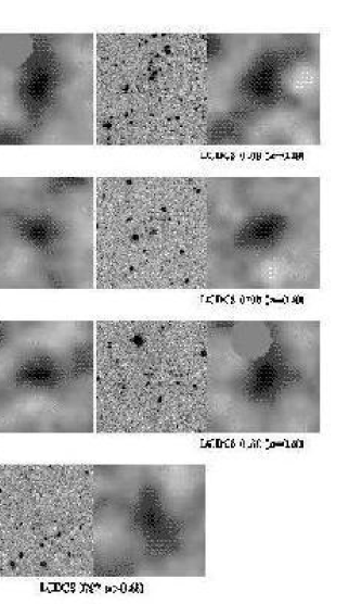
Figure 1.: Examples of candidate clusters. Left panel shows the original survey data, right panel has the cleaned and smoothed version. Estimated redshifts range from 0.3 for the upper left to $>$ 0.85 for the lowest panel. The intermediate step where resolved galaxies and stars are removed is not shown. The LSB fluctuation does not arise from the resolved sources visible in the left panels.

3. Follow-Up Observations

The telescope-intensive part of the project has been the follow-up observations necessary to test our cluster candidates and calibrate the methods we are using to estimate the cluster redshift and mass (see below). Such expensive follow-up methods are common to all surveys regardless of whether they originate from optical, X-ray, or SZ data. We now describe some of the observations that lead us to conclude that the overall contamination of the cluster catalog is $\sim$ 30% (with greater contamination toward higher redshifts). While X-ray and SZ surveys should have lower contamination rates, optical follow-up will still be necessary at least for redshift determination.

3.1. Photometry

A basic method to confirm cluster candidates is to obtain deeper images that enable one to identify a concentration of galaxies at the position of the LSB fluctuation and a red galaxy sequence in color-magnitude diagrams characteristic of early-type galaxies in clusters. We show examples of these two approaches using data presented by Nelson et al (2001). First, in Figure 1 we plot the radial density of galaxies in cluster candidates that we have deemed to be bona-fide. There is a clear central concentration of galaxies indicative of a cluster. Second, in Figure 2 we plot the color of the red sequence vs. spectroscopic redshift (see below) for clusters from our survey vs. clusters from the literature (some of our cluster candidates come from an exploratory survey done using Palomar 5m drift scans; Dalcanton et al. 1997). The excellent agreement between the two samples is indicative that the objects that we call clusters (not all candidates, but rather those $\sim$ 70% that we deem to be bona-fide clusters) are indeed similar to cluster in the literature. Finally, we plot the results from recent VLT observations for an ongoing program that aims to investigate the detailed properties of 10 clusters at $z\sim 0.5$ and another 10 at $z\sim 0.8$. These data come from the initial snapshots intended to confirm clusters candidates before more observing time is spent. Here we include all of the $z\sim 0.5$ candidates (regardless of whether in the final analysis we deem them to be bona-fide). Red sequences are prominent in the majority, again confirming that the contamination rate is not significantly larger than 30%.

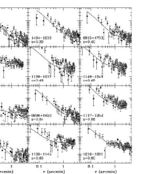
Figure 2.: Radial profiles of a sample of “confirmed” cluster candidates.

3.2. Spectroscopy

Complementary confirming evidence comes from spectroscopy. In Figure 4 we present all of our spectroscopic follow-up data from the Keck telescopes. The spectrograph slit was placed at the position of the LSB feature identified in the original survey data and the guider was used to rotate the slit in such a way as to include as many galaxies as possible. The groupings in redshift space of three or more galaxies that resulted from these observations in the majority of the cluster candidate fields again confirms our contamination rate. Monte-Carlo simulations using Keck field redshift surveys to similar magnitudes suggest that our spectroscopic sample could include one random three galaxy grouping and no random four galaxy groupings. Some of the failed cluster candidates may actually be clusters because 1) we may have been unfortunate in our placement of the spectrograph slit and simply missed including enough cluster galaxies, and 2) some of the failed candidate fields received substandard exposures (due to time constrains or weather).

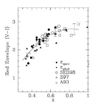
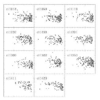
Figure 3.: Photometric confirmation. Left panel plots the color of the red sequence for our clusters (solid symbols) vs. literature cluster (open symbols). The line represents an empirical fit the the color vs. redshift relation (see Nelson et al. 2001 for a full description). The right panel shows color-magnitude diagrams from VLT snapshot exposures of $z\sim 0.5$ candidate clusters.

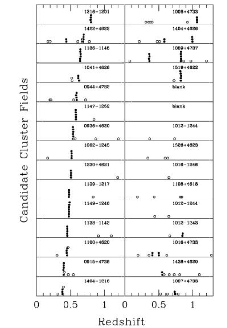
Figure 4.: Spectroscopic follow-up of cluster candidates. Each panel represents one cluster candidate field. In each panel, the filled circles represent galaxies within 1000 km sec^-1 of another galaxy and open circles represent other galaxies. The two empty panels are not candidate cluster fields. The candidates are sorted into two groups (likely clusters and unlikely clusters) and within the former group by redshift.

4. Calibrating Redshift and Mass Diagnostics

In surveys that produce thousands (or even hundreds) of galaxy cluster identifications, it is impractical to obtain redshift and mass measures via spectroscopy for a significant fraction of the candidates. Ideally, these quantities should be estimated from the survey data themselves. As such, we clearly sacrifice precision on a cluster-by-cluster basis, but if the uncertainties are well understood, the sheer number of clusters allows high precision measures of the statistical properties of the sample. There really is no choice in this matter (in this survey or future SZ surveys). For example, to obtain a sufficient number of spectroscopic redshifts of cluster galaxies for a reliable velocity dispersion measure ($\sim$ 50) in a sample of ONLY 20 clusters we require $\sim$ 35 VLT nights!

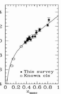
Figure 5.: BCG magnitudes vs. redshifts. The open circles represent known foreground clusters that lie within our survey. $m_{W}$ is the galaxy magnitude for the wide optical filter used in the survey.

We use the magnitude of the brightest cluster galaxy (BCG) as a redshift indicator and the central surface brightness of the smoothed cluster detection ($\Sigma$) as a mass indicator. BCGs are excellent standard candles locally (Humason, Mayall, & Sandage 1956; Graham et al. 1996) and at high redshift (Aragon-Salamanca et al. 1993.). In Figure 5 we show our empirical calibration of the BCG magnitudes in our photometric system vs. spectroscopic redshift (as obtained for the cluster from the Keck data). The dispersion is $\sim 0.08$ in $z$ once a correction is applied to the BCG magnitude for cluster mass (again empirically calibrated from the data). However, the redshift error distribution is non-Gaussian and we construct the full distribution by randomly inserting cluster candidates into the original survey images and reanalyzing them (see Gonzalez et al. (2001) for a full description).

The calibration of the mass indicator is much more speculative primarily because of the dearth of independent mass estimates for high redshift clusters. Only one previously known X-ray cluster at $z>0.35$ lies within our survey area, so we obtained small drift scans around 17 other clusters with published X-ray luminosity and/or temperature measurements. Nevertheless, the relationships between $\Sigma$ and other mass indicators ($L_{x},T_{x},$ or velocity dispersion) are poorly defined. Two aspects are particularly vexing: 1) we need to determine not only the relation between these quantities but we also need to quantify the scatter, and 2) most of the data are for lower redshift clusters, complicating the removal of redshift-dependent effects like evolution. Extracting the full potential of this, or any other survey, is predicated on developing a reliable mass estimator and understanding its uncertainties.

5. The Correlation Function of Clusters

As an example of statistical results that can be obtained from our cluster catalog we briefly discuss our first result regarding large-scale structure. The cluster-cluster correlation function has a complicated history that cannot be outlined here. However, it is generally parametrized by examining the behavior of the correlation scale-length, $r_{0}$, vs. the mean cluster separation of a sample, $d_{c}$. The latter is a measure of the mass of the clusters because more massive clusters are rarer and so have larger mean cluster separations.

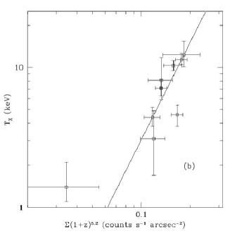
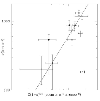
Figure 6.: X-ray temperature and galaxy velocity dispersion vs. $\Sigma$ (corrected for cosmological dimming and evolution empirically)

We select a subsample in the redshift range where we believe our contamination is lowest and best understood ($0.35<z<0.6$), and for which our redshift and mass estimates are more robust. We invert the Limber equation to convert the angular correlation function into a spatial function. The comparison of our results with those from local ($z<0.2$) surveys and simulations is presented in Figure 7. We find that the correlation of clusters at $z\sim 0.5$ is quite similar to that seen at lower redshifts. The low redshift results agree with the predictions from the VIRGO consortium simulation (Colberg et al. 2000) and with the very moderate amount of evolution expected theoretically. This measure of large-scale structure is not a particularly powerful discriminator amongst the currently allowed cosmological models, but the results demonstrate that our measured clusters at intermediate redshifts are consistent with our current theoretical understanding.

6. Conclusions

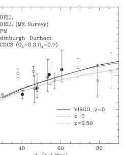
Figure 7.: Correlation scale-length vs. mean cluster separation. Solid line represents results from VIRGO simulations at $z=0$ and the dotted line represents theoretical expectation for $z=0.5$.

The Las Campanas Distant Cluster Survey provides another view on cluster selection and so complements not only other optical surveys, but surveys at other wavelengths. Every method has potential systematic problems, and rather than promoting one method over the others, we encourage cross-comparison of the various methods to identify and resolve those problems. To that aim, 1) we have published our catalog (Gonzalez et al. 2001), 2) we have targeted 18 X-ray clusters and recovered all but one, which is at low Galactic latitude, thereby demonstrating that our false negative rate with respect to bona-fide X-ray clusters is low, 3) begun a weak-lensing analysis of 20 of our candidates (the only one analyzed to date by D. Clowe shows a significant mass signature, as does a less massive candidate cluster in the same field) and 4) are in the process of obtaining Chandra data for four candidates. SZ observations of some of these clusters would add significantly to our understanding of the selection function.

The study of clusters has entered a new era where large samples of candidate clusters are becoming common. It becomes increasingly important to acknowledge that the detailed studies of clusters as done when only a few clusters where available does not fully exploit the power of these large samples. We have begun to develop redshift and mass estimators from our survey data and apply them to produce statistical results obtained from the entire catalog. Future work must focus on refining these calibrations. We are no longer limited by cluster statistics, but we remain limited by systematic uncertainties.

Acknowledgments.

DZ acknowledges financial support from the David and Lucile Packard Foundation, the Sloan Foundation, the NSF CAREER program (AST 97-33111), and the conference organizers. Data fron the ESO distant cluster survey obtained from the ESO NTT and VLT telescopes.

References

Aragon-Salamanca, A., Ellis, R.S., Couch, W.J., & Carter, D. 1993, MNRAS, 262, 764

Colberg, J.M, et al. 2000, MNRAS, 319, 209

Dalcanton, J.J., 1996, ApJ, 466, 92

Dalcanton, J.J., Spergel, D.N., Gunn, J.E., Schmidt, M., & Schneider, D.P. 1997, AJ, 114, 635

Gonzalez, A.H., Zaritsky, D., Dalcanton, J.J., & Nelson, A.E., 2001, ApJS, in press

Gonzalez, A.H., Zaritsky, D., Wechsler, R., 2001, ApJL, submitted

Graham, A., Lauer, T.R., Colless, M., & Postman, M. 1996, ApJ, 465, 534

Humason, M.L., Mayall, N.U., & Sandage, A.R. 1956, AJ, 61, 97

Nelson, A.E., Gonzalez, A.H., Zaritsky, D., & Dalcanton, J.J., 2001, ApJ, submitted

Zaritsky, D., Nelson, A.E., Dalcanton, J.J., & Gonzalez, A.H., 1997, ApJL, 480, L91

Zaritsky, D., Shectman, S.A., & Bredthauer, G. 1996, PASP, 108, 104