The Effect of a Binary Source Companion on the Astrometric Microlensing Behavior

Abstract

If gravitational microlensing occurs in a binary-source system, both source components are magnified, and the resulting light curve deviates from the standard one of a single source event. However, in most cases only one source component is highly magnified and the other component (the companion) can be treated as a simple blending source: blending approximation. In this paper, we show that, unlike the light curves, the astrometric curves, representing the trajectories of the source image centroid, of an important fraction of binary-source events will not be sufficiently well modeled by the blending effect alone. This is because the centroid shift induced by the source companion endures to considerable distances from the lens. Therefore, in determining the lens parameters from astrometric curves to be measured by future high-precision astrometric instruments, it will be important to take the full effect of the source companion into consideration.

1 Introduction

If microlensing occurs in a binary-source system, both source components are gravitationally magnified and the resulting light curve deviates from the standard one of a single source event (Griest & Hu 1992; Han & Gould 1997). However, the photometric binary-source effect becomes important only for the rare cases of the lens trajectory’s passage close to both source stars and in most cases only one source component is significantly magnified. Then, the less magnified source component (the companion) can be treated simply as a blending source, and the resulting light curve may then be approximated by that of a blended single source event (Dominik 1998).

Although microlensing events have till now been observed only photometrically (Alcock et al. 1993; Aubourg et al. 1993, Udalski et al. 1993; Alard & Guibert 1997; Abe et al. 1997), they could also be observed astrometrically by using high-precision instruments that will become available in the near future, e.g. the Space Interferometry Mission (SIM, Unwin et al. 1998), and the interferometers to be mounted on the Keck (Colavita et al. 1998) and VLT (Mariotti et al. 1998). If an event is astrometrically observed, one can measure the displacements in the source star image centeroid with respect to its unlensed position. Once the trajectory of the centroid shifts (the astrometric curve) is measured, the physical parameters (mass and location) of the lens can be better constrained (Miyamoto & Yoshii 1995; Høg, Novikov & Polnarev 1995; Walker 1995; Boden, Shao & Van Buren 1998; Han & Chang 1999).

The binary source companion also affects the astrometric lensing behavior. However, whenever its astrometric effect was considered (Han & Kim 1999; Dalal & Griest 2001), it was always treated as a simple blending source due to the belief that the astrometric binary-source effect would be similar to the photometric one. In this paper, we show that contrary to this belief the effect of the source companion on the astrometric lensing behaviors of a significant fraction of binary-source events cannot be sufficiently well described by the blending approximation, even when the corresponding light curves are well approximated by the blending effect alone.

The paper is organized as follows. In § 2, we describe the basics of binary source and blending effects on the light and astrometric curves of lensing events. In § 3, we the present astrometric curves and the corresponding light curves of example binary-source events to illustrate the relative difficulty in describing the astrometric lensing behaviors by the blending approximation alone. In § 4, we statistically estimate the range of the binary source separation and the companion light fraction where the blending approximation breaks down for the description of the photometric and astrometric lensing behaviors. We conclude with § 5.

2 Binary source and Blending Effects

2.1 Binary Source Effect

When a single source is lensed, its image is split into two. The two images appear at the positions

$$\mbox{\boldmath$\theta$}_{{\rm I}\pm}={\theta_{\rm E}\over 2}\left(u\pm\sqrt{u^{2}+4}\right)\hat{\mbox{\boldmath$u$}},$$ (1)

and have magnifications

$$A_{\pm}={1\over 2}\left({u^{2}+2\over u\sqrt{u^{2}+4}}\ \pm 1\right),$$ (2)

where $\theta_{\rm E}$ is the angular Einstein ring radius, $u$ is the lens-source separation vector normalized by $\theta_{\rm E}$, and $\hat{\mbox{\boldmath$u$}}$ represents its unit vector. The angular Einstein ring radius is related to the physical parameters of the lens by

$$\theta_{\rm E}=\sqrt{4Gm\over c^{2}}\left({1\over D_{\rm ol}}-{1\over D_{\rm os}}\right)^{1/2},$$ (3)

where $m$ is the lens mass and $D_{\rm ol}$ and $D_{\rm os}$ represent the distances to the lens and source star, respectively. The lens-source separation vector is related to the lensing parameters by

$$\mbox{\boldmath$u$}=\left({t-t_{0}\over t_{\rm E}}\right)\ \hat{\mbox{\boldmath$x$}}+\beta\ \hat{\mbox{\boldmath$y$}},$$ (4)

where $t_{\rm E}$ represents the time required for the source to transit $\theta_{\rm E}$ (Einstein time scale), $\beta$ is the closest lens-source separation in units of $\theta_{\rm E}$ (impact parameter), $t_{0}$ is the time at that moment, and the unit vectors $\hat{\mbox{\boldmath$x$}}$ and $\hat{\mbox{\boldmath$y$}}$ are parallel with and normal to the direction of the lens-source motion. The two images formed by the lens cannot be resolved, but one can measure the total magnification and the shift of the light centroid of the source star with respect to its unlensed position, which are represented respectively by

$$A=A_{+}+A_{-}={u^{2}+2\over u\sqrt{u^{2}+4}},$$ (5)

and

$$\mbox{\boldmath$\delta$}={A_{+}\mbox{\boldmath$\theta$}_{{\rm I}+}+A_{-}\mbox{\boldmath$\theta$}_{{\rm I}-}\over A}-\mbox{\boldmath$u$}={\mbox{\boldmath$u$}\over u^{2}+2}\theta_{\rm E}.$$ (6)

The resulting light curve is symmetric with respect to $t_{0}$ and the trajectory of the centroid shift traces an ellipse with a semi-major axis $a=(\beta^{2}+2)^{-1/2}\theta_{\rm E}/2$ and an axis ratio $q=\beta(\beta^{2}+2)^{-1/2}$ (Walker 1995; Jeong, Han & Park 1999).

If lensing occurs in a binary-source system, on the other hand, both source components are gravitationally magnified. For the binary-source event, the lensing behavior involved with each source can be treated as an independent single source event. Then the observed light and astrometric curves are represented by

$$F_{\rm BS}=A_{1}F_{1}+A_{2}F_{2},$$ (7)

and

$$\mbox{\boldmath$\delta$}_{\rm BS}={A_{1}F_{1}(\mbox{\boldmath$u$}_{1}+\mbox{\boldmath$\delta$}_{1})+A_{2}F_{2}(\mbox{\boldmath$u$}_{2}+\mbox{\boldmath$\delta$}_{2})\over A_{1}F_{1}+A_{2}F_{2}}-{F_{1}\mbox{\boldmath$u$}_{1}+F_{2}\mbox{\boldmath$u$}_{2}\over F_{1}+F_{2}},$$ (8)

where $\mbox{\boldmath$u$}_{i}$ are the separation vectors between the lens and the individual source components, $A_{i}$ and $\mbox{\boldmath$\delta$}_{i}$ are the magnifications and the centroid shifts of the individual single source events with baseline source fluxes $F_{i}$, and the subscripts $i=1$ and 2 are used to denote parameters related to the individual single source events ($i=1$ for the event with the higher magnification). We note that the reference position of the centroid shift measurements for the binary-source event is not the location of the primary, i.e. $\mbox{\boldmath$u$}_{1}$, but the center of light between the unlensed source components, i.e. the second term in eq. (8). In Figure 1, we present the lens system geometry of an example binary-source event.

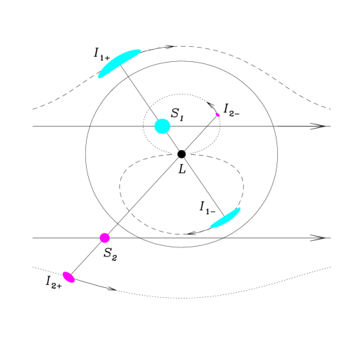
Figure 1: The lens system geometry of an example binary-source event. The lens (denoted by ‘L’) is located at the center of the Einstein ring (large circle). The two small filled circles (denoted by ‘$S_{i}$’, where $i=1$ and 2) represent the locations of the two source stars at a specific moment. The two distorted figures (denoted by ‘$I_{i+}$’ and ‘$I_{i-}$’) located along the line connecting each source and the lens are the images corresponding to the individual source stars. The straight lines with arrows represent the source trajectories. The curve passing through each image and the arrow on it represent the trajectory and direction of the image motion.

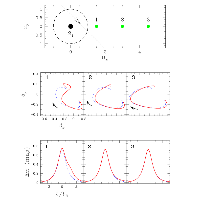
Figure 2: Astrometric and light curves of binary-source events and in comparison with those obtained by the blending approximation. The upper panel shows the geometry of the lens systems, where the primary (denoted by ‘$S_{1}$’) is located at the origin and the dots (designated by numbers) on the right side are the three different locations of the companion. The straight line with an arrow represents the lens trajectory. The dashed circle represents the lens locations where the magnification of the primary source is $A_{1}=3/\sqrt{5}\sim 1.34$. The middle and lower panels show how the astrometric and light curves change with the increasing source separation. The number on each panel corresponds to that designating the companion location. The solid curves are the exact astrometric and light curves of the binary-source events, and the dotted curves are those obtained by the blending approximation. The companion has a light fraction of $f=0.2$.

2.2 Blending Effect

If a single source event is affected by the blended light from an unresolved nearby star, the observed light curve is represented by

$$F_{\rm blend}=AF_{0}+F_{\rm b},$$ (9)

where $F_{0}$ is the unblended baseline source flux and $F_{\rm b}$ is the amount of blended flux. Since $F_{\rm b}$ is constant throughout the event, the observed flux is uniformly increased by $F_{\rm b}$ and the shape of the light curve is still symmetric.

The centroid shift of a blended event is represented by

$$\mbox{\boldmath$\delta$}_{\rm blend}={AF_{0}(\mbox{\boldmath$u$}+\mbox{\boldmath$\delta$})+F_{b}\mbox{\boldmath$u$}_{\rm b}\over AF_{0}+F_{\rm b}}-{F_{0}\mbox{\boldmath$u$}+F_{\rm b}\mbox{\boldmath$u$}_{\rm b}\over F_{0}+F_{\rm b}},$$ (10)

where $\mbox{\boldmath$u$}_{\rm b}$ is the position vector of the blending source with respect to the lens (Han & Kim 1999; Dalal & Griest 2001). Blending has two effects on the observed astrometric curve. Firstly, it causes the source star image centroid to be additionally shifted towards the blending source during the event. Secondly, due to blending, the reference position of the centroid shift measurements is no longer the position of the lensed source but the center of light between the lensed star and the blending source. As a result, depending on the position and the light fraction of the blending source, $f=F_{\rm b}/(F_{0}+F_{\rm b})$, the resulting astrometric curves can be seriously distorted from the elliptical one of the unblended event (Han & Kim 1999; Dalal & Griest 2001).

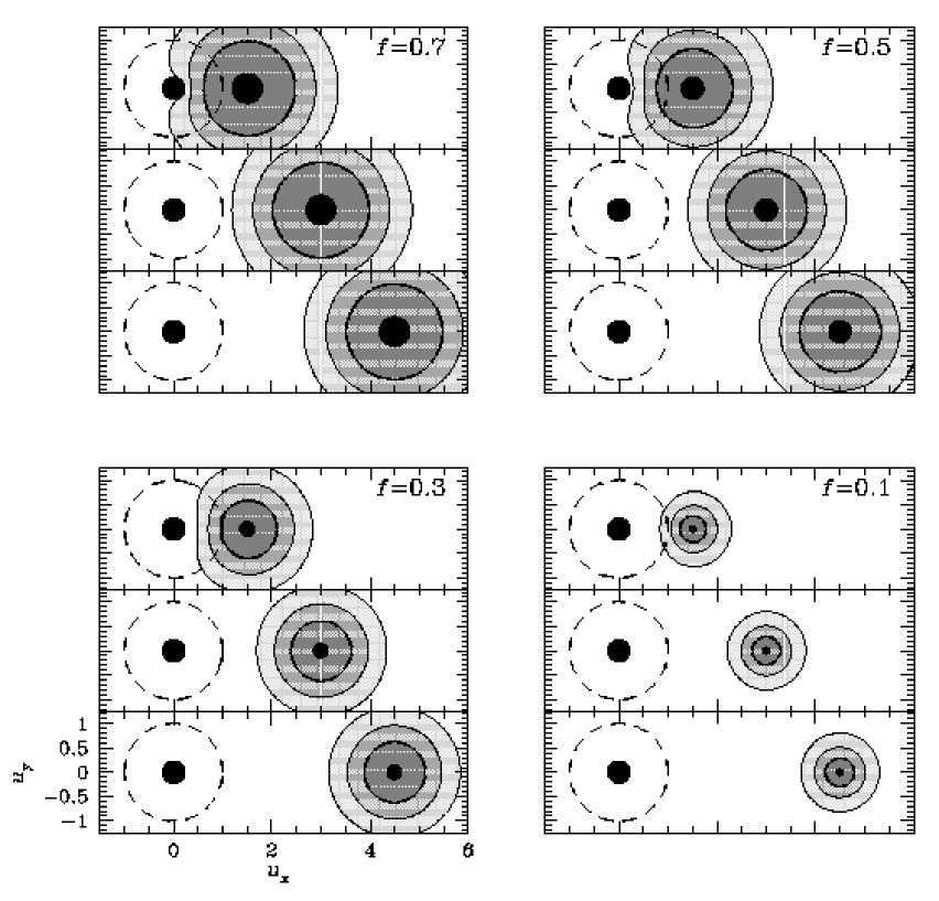
Figure 3: Contour maps of binary source magnification excesses from the blending approximation. The individual sets of panels are the maps of binary source systems with different companion light fractions. The panels in each set show the variation of the excess pattern with increasing source separation. Contours are drawn at the levels of $\epsilon=5\%$, 10%, and 20%, respectively.

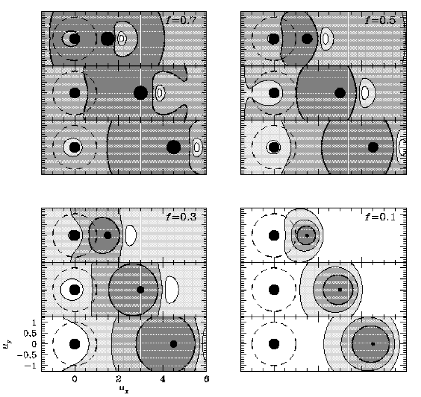
Figure 4: Similar maps as in Fig. 3, but for the astrometric centroid shift excesses $\Delta\delta$. Contours are drawn at the levels of $\Delta\delta=0.05\theta_{\rm E}$, $0.1\theta_{\rm E}$, and $0.2\theta_{\rm E}$, respectively.

3 Blending Approximation

In many cases, the light curves of binary-source events resemble those of single source events. This is because the lens, in general, approaches closely only one of the source components. In this case, the magnification of the companion is small, i.e. $A_{2}\sim 1.0$, and thus the the resulting light curve can be approximated as

$$A_{\rm BS}\sim A_{1}F_{1}+F_{2}.$$ (11)

This implies that the observed light curve is well described by that of a single source event where the companion simply acts as a blending source.

Can the blending approximation be equally applied to astrometric curves of most binary-source events? To this question, we find the answer is ‘no’. We demonstrate this in Figure 2, where we present the astrometric (middle panels) and light curves (lower panels) of binary-source events with three different values of source separation, and we compare these curves to those obtained by the blending approximation. One finds that even when the light curve is well approximated by the blending effect alone, the deviation of the astrometric curve from the approximation is considerable.

To see the patterns of both the photometric and astrometric deviations from the blending approximation for more general cases of binary-source events, we construct contour maps of magnification and centroid shift excesses for binary-source systems with various values of the binary separation, $\ell$, and the companion light fraction, $f$. The magnification and centroid shift excesses are defined respectively by

$$\epsilon={A_{\rm BS}-A_{\rm blend}\over A_{\rm blend}},$$ (12)

and

$$\Delta\mbox{\boldmath$\delta$}=\mbox{\boldmath$\delta$}_{\rm BS}-\mbox{\boldmath$\delta$}_{\rm blend},$$ (13)

where $A_{\rm BS}$ and $\mbox{\boldmath$\delta$}_{\rm BS}$ are the exact magnification and centroid shift of the binary-source event, and $A_{\rm blend}$ and $\mbox{\boldmath$\delta$}_{\rm blend}$ are those obtained by the blending approximation. The constructed maps are presented in Figure 3 for the excess magnification, and in Figure 4 for the excess centroid shift, respectively. From a comparison of the two maps, one finds that while significant photometric deviations occur only in a small region around the companion, comparable astrometric deviations occur in a substantially larger area, even for a companion with a large separation and a small light fraction.

The relative difficulty in describing the astrometric curves of binary-source events by just the blending approximation can be understood in the following way. If a source companion is located at a large distance from the lens (i.e. $u_{\rm 2}\gg\sqrt{2}$), its contribution to the magnification and the centroid shift are represented by

$$A_{2}\sim 1+{2\over u_{2}^{4}},$$ (14)

and

$$\delta_{2}\sim{\theta_{\rm E}\over u_{2}}.$$ (15)

Then, as the separation becomes larger, the photometric contribution falls off rapidly ($\sim u_{2}^{4}$), while the astrometric contribution decays much more slowly ($\sim u_{2}$) (Miralda-Escudé 1996; Paczyński 1998). As a result, even at the location where the magnification of the companion is negligible (i.e. $A_{2}\sim 1$), the amount of the centroid shift can be considerable. In this range of $u_{\rm 2}$, the centroid shift becomes

$$\mbox{\boldmath$\delta$}_{\rm BS}\sim{A_{1}F_{1}(\mbox{\boldmath$u$}_{1}+\mbox{\boldmath$\delta$}_{1})+F_{2}(\mbox{\boldmath$u$}_{2}+\mbox{\boldmath$\delta$}_{2})\over A_{1}F_{1}+F_{2}}-{F_{1}\mbox{\boldmath$u$}_{1}+F_{2}\mbox{\boldmath$u$}_{2}\over F_{1}+F_{2}},$$ (16)

which differs from $\mbox{\boldmath$\delta$}_{\rm blend}$ in eq. (10).

4 Validity of the Blending Approximation

In the previous section, we illustrated the relative difficulties in describing the astrometric lensing behavior of binary-source events by the blending approximation, as compared to the photometric behavior. Then, a natural question to ask is: over what range of values of the source separation and the companion light fraction does the blending approximation break down for the description of the photometric and astrometric behaviors of binary-source events? We answer this question as follows.

We proceed by statistically estimating the probabilities of binary-source events whose light and astrometric curves can be approximated by the blending effect as functions of $\ell$ and $f$; $P_{\rm ph}(\ell,f)$ for the photometric and $P_{\rm ast}(\ell,f)$ for the astrometric measurements. To determine these probabilities, we first simulate a large number of microlensing events occurred in binary-source systems, characterized by $\ell$ and $f$. We then determine the probabilities by estimating the fraction of events whose light and astrometric curves have deviations (from those obtained by the blending approximation) less than preselected threshold values. The lens trajectories of the tested events are selected so that they have random orientations with respect to the binary axis, and so that their impact parameters with respect to the primary source are uniformly distributed in the range of $0\leq\beta_{1}\leq 1$. We assume that the blending approximation is valid if the light and astrometric curves, measured during the time period $-10t_{\rm E}\leq t\leq 10t_{\rm E}$, have deviations less than the threshold values of $\epsilon_{\rm th}=10\%$ and $\Delta\delta_{\rm th}=0.1\theta_{\rm E}$, respectively.

Figure 5: The probabilities of binary-source events whose light and astrometric curves can be approximated by the blending well approximation, as functions of the binary separation, $\ell$, and the companion light fraction, $f$. The upper and lower panels are for the photometric and astrometric probabilities, respectively.

In Figure 5, we present the resulting probabilities as contour maps in the parameter space of $\ell$ and $f$: upper panel for $P_{\rm ast}(\ell,f)$ and lower panel for $P_{\rm ast}(\ell,f)$. From the figure, one finds that for a given $\ell$ and $f$, $P_{\rm ast}$ is significantly lower than the corresponding $P_{\rm ph}$. For example, if microlensing occurs in a binary-source system with $\ell=6.0\theta_{\rm E}$, we estimate that the probabilities of events whose astrometric curves can be treated by the blending approximation will be only $P_{\rm ast}\sim 0\%$, 20%, 50%, and 70% for companions with light fractions of $f=0.8$, 0.6, 0.4, and 0.2, respectively; while the corresponding photometric probabilities will be $P_{\rm ph}\mathrel{\hbox{\hbox to0.0pt{\hbox{\lower 4.0pt\hbox{$\sim$}}\hss}\hbox{$>$}}}80\%$ for all four values of $f$. One also finds that the region of low $P_{\rm ast}$ occupies a significantly larger area in the parameter space than the low $P_{\rm ph}$ region, implying that the astrometric blending approximation will not be valid for a significant fraction of binary-source events.

5 Conclusion

We have shown that although the blending approximation describes well the photometric lensing behaviors of most binary-source events, the approximation will not be able to adequately describe the astrometric lensing behaviors for a significant fraction of binary-source events. This is because the astrometric effect of the companion endures to relatively large distances where the corresponding photometric effect is negligible. Therefore, it will be important to take the full effect of the binary companion into consideration in determining the lens parameters from the observed source motion.

We thank André Fletcher (Korea Astronomy Observatory) for his help with the preparation of the paper. This work was supported by a grant (1999-2-1-13-001-5) from the Korea Science & Engineering Foundation (KOSEF).

References

- [1] Abe F., et al., 1997, in Variable Stars and Astrophysical Returns of Microlensing Surveys, eds. R. Ferlet, J.-P. Milliard & B. Raba (Cedex: Editions Frontiers), 75
- [2] Alard C., Guibert J., 1997, A&A, 326, 1
- [3] Alcock C., et al., 1993, Nature, 365, 621
- [4] Aubourg E., et al., 1993, Nature, 365, 623
- [5] Boden A. F., Shao M., Van Buren D., 1998, ApJ, 502, 538
- [6] Colavita M. M., et al., 1998, Proc. SPIE, 3350-31, 776
- [7] Dalal N., Griest K., 2001, preprint (astro-ph/0101217)
- [8] Dominik M., 1998, A&A, 333, 893
- [9] Griest K., Hu W., 1992, ApJ, 397, 362
- [10] Jeong Y., Han C., Park S.-H., 1999, ApJ, 511, 569
- [11] Han C., Chang K., 1999, MNRAS, 304, 845
- [12] Han C., Gould A., 1997, ApJ, 480, 196
- [13] Han C., Jeong Y., 1998, MNRAS, 301, 231
- [14] Han C., Kim T.-W., 1999, MNRAS, 305, 795
- [15] Høg E., Novikov I. D., Polnarev A. G., 1995, A&A, 294, 287
- [16] Mariotti J. M., et al., 1998, Proc. SPIE, 3350-33, 800
- [17] Miralda-Escudé J., 1996, ApJ, 470, L113
- [18] Miyamoto M., Yoshii Y., 1995, AJ, 110, 1427
- [19] Paczyński B., 1998, ApJ, 494, L23
- [20] Udalski A., Szymański M., Kaluzny J., Kubiak M., Krzemiński W., Mateo M., Preston G. W., Paczyński B., 1993, Acta Astron., 43, 289
- [21] Unwin S., Boden A., Shao M., 1997, in AIP Conf. Proc. 387, Space Technology and Applications International Forum 1997, eds. El-Genk (New York: AIP), 63
- [22] Walker M. A., 1995, ApJ, 453, 37