Galaxy Correlation Statistics of Mock Catalogs for the DEEP2 Survey

Abstract

The DEEP2 project will obtain redshifts for $\sim$60,000 galaxies between $z\simeq$ 0.7–1.5 in a comoving volume of roughly 7 10⁶ Mpc³ $h^{-3}$ for a $\Lambda$CDM universe. The survey will map four separate 2^∘ by 0.5^∘ strips of the sky. To study the expected clustering within the survey volume, we have constructed mock galaxy catalogs from the GIF and Hubble Volume simulations developed by the Virgo consortium. We present two- and three-point correlation analyses of these mock galaxy catalogs to test how well we will measure these statistics, particularly in the presence of selection biases which will limit the surface density of galaxies which we can select for spectroscopy. We find that although the projected angular two-point correlation function $w(\theta)$ is strongly affected, neither the two-point nor three-point correlation functions, $\xi(r)$ and $\zeta(r)$, are significantly compromised. We will be able to make simple corrections to account for the small amount of bias introduced. We quantify the expected redshift distortions due to random orbital velocities of galaxies within groups and clusters (“fingers of god”) on small scales of $\sim$1 Mpc $h^{-1}$ using the pairwise velocity dispersion $\sigma_{12}$ and galaxy-weighted velocity dispersion $\sigma_{1}$. We are able to measure $\sigma_{1}$ to a precision of $\sim$10%. We also estimate the expected large-scale coherent infall of galaxies due to supercluster formation (“Kaiser effect”), as determined by the quadrupole-to-monopole ratio $\xi_{2}$/$\xi_{0}$ of $\xi(r_{p},\pi)$. From this measure we will be able to constrain $\beta$ to within $\sim$0.1 at $z$=1.

For the DEEP2 survey we will combine the correlation statistics with galaxy observables such as spectral type, morphology, absolute luminosity, and linewidth to enable a measure of the relative biases in different galaxy types. Here we use a counts-in-cells analysis to measure $\sigma_{8}$ as a function of redshift and determine the relative bias between galaxy samples based on absolute luminosity. We expect to measure $\sigma_{8}$ to within 10% and detect the evolution of relative bias with redshift at the 4–5$\sigma$ level, with more precise measurements for the brighter galaxies in our survey.

1 INTRODUCTION

The DEEP2 survey (Davis et al., 2000) will commence in the spring of 2002, with the anticipated delivery of the DEIMOS spectrograph (Cowley et al., 1997) to Keck in the fall of 2001. The survey will use approximately 120 Keck nights over a period of three years to study galaxy properties, evolution, and large-scale structure at $z\sim$ 1. The DEEP2 survey will obtain spectra for $\sim$60,000 galaxies between $z\approx$ 0.7–1.5. The current plan is to use an 830 l mm^-1 grating with 0.75 $\arcsec$ slitwidths, resulting in a spectral resolution of 86 km s^-1. We thus expect to easily measure linewidths to this limit and redshifts to 10% of this limit. The survey will target four 2^∘ by 0.5^∘ fields, which corresponds to a total comoving area of 80 by 20 $h^{-2}$ Mpc² at $z\sim$ 1 for a $\Lambda$CDM universe. The line-of-sight comoving distance for $z\approx$ 0.7–1.5 is $\sim$1400 $h^{-1}$ Mpc, though in our magnitude-limited survey we will not sample the higher-redshift region very densely. The four fields were chosen as low-extinction regions which are continuously observable from Hawaii over a six month interval. One field is the Groth Survey strip, and two fields are on the equatorial strip which will be deeply imaged by the Sloan Digital Sky Survey (SDSS). Each of these fields are targets of a CFHT survey conducted by Kaiser and Luppino, with the primary goal of deep imaging in B, R, and I bands for weak lensing studies (Wilson et al., 2000). We will use their photometric information to color-select galaxies with $z\geq$ 0.7 and $m_{I}(AB)\leq$ 23.5 for the DEEP2 survey. This color-selection allows us to focus on the high-$z$ universe.

One of the key science goals of the DEEP2 survey is to measure the two-point and higher-order correlation functions of galaxies at $z\sim$ 1 as a function of other observables. In almost all models of structure formation (e.g., White, Davis, Efstathiou, & Frenk (1987)), galaxies are born as highly biased tracers of the mass distribution, but their bias diminishes with time. Spiral galaxies today appear to be weakly biased, if at all, while the clustering of $z\sim$ 3 Lyman-break galaxies requires a large bias for any reasonable cosmological model (Giavalisco et al., 1998; Wechsler et al., 1998). Galaxies at $z\sim$ 1 should have an intermediate degree of bias, with readily observable consequences.

The statistical clustering of galaxies at any epoch depends on both the underlying dark matter distribution and the biasing function; the two are degenerate without more information. However, models suggest that patterns exist in the relative biases between various types of galaxies, and measuring these patterns as a function of absolute luminosity, linewidth, or spectral type can break that degeneracy. With sufficiently dense sampling, determining the clustering properties of galaxies can yield direct measurements of their biasing. For example, in linear biasing models [where $(\delta\rho/\rho)_{gal}$ is assumed to be some constant $b\times(\delta\rho/\rho)_{mat}$], the mean ratio of the skewness of the density distribution function to the square of its variance has an expectation value that scales as $1/b$ (Fry, 1996; Scoccimarro et al., 1998). We will be able to subdivide the DEEP2 sample as a function of internal linewidth and estimate $b$ for each type of galaxy. The sampling density of the survey is such that we will be able to obtain spectra for three-quarters of all galaxies down to $L^{*}+0.5$ at the redshifts of interest. Comparison of such measures at $z\sim 1$ to their values at $z=0$ will then be possible.

DEIMOS has a field of view of 16$\arcmin$ by 5$\arcmin$ for both imaging and multislit spectroscopy and will use an array of eight 2k by 4k Lincoln Laboratory 30 $\micron$ thick CCDs, with an active 2-D flexure compensation system to minimize fringing at red wavelengths. As the DEEP2 survey will target four fields of 120$\arcmin$ by 30$\arcmin$, slitmasks will be made from a region of size 16$\arcmin$ by 4$\arcmin$ with two rows of 60 masks each. There will be $\sim$130 slitlets per mask, with most of the slitlets aligned along the long axis, but with some tilted as much as $30^{\circ}$ to track extended galaxies in order to measure rotation curves. The mean surface density of candidate galaxies exceeds the number of objects we can select, and spectra of selected targets cannot be allowed to overlap on the CCD. Adjacent slitmasks will overlap by 2 $\arcmin$ so that each galaxy will have two chances to be selected for a mask. Spectra will be obtained for $\sim$70$\%$ of the targeted galaxies in the fields meeting our color and magnitude selection criteria, chosen by a slitmask algorithm which is necessarily biased against the highest-density regions, where the spectra of nearby galaxies would overlap on the CCD. Here we test how this bias will affect our measurement of the underlying two-point and three-point correlation functions.

This paper uses a family of mock catalogs to model large-scale structure studies that will be possible with the DEEP2 survey data. Section 2 describes the construction of the mock catalogs while section 3.1 provides results of analysis of two-point correlation studies in $\xi(r_{p},\pi)$. The high resolution spectroscopy of DEEP2 will allow redshift space distortions to be readily measured, as discussed in section 3.2. This in turn will allow for a measurement of the small-scale thermal velocities $\sigma_{12}$ and $\sigma_{1}$, described in section 3.3. In section 3.4 we show that we can measure the three-point correlation function $\zeta(r)$ with minimal bias. Section 3.5 discusses the ability to measure the evolution of clustering within the volume of the DEEP2 survey. We expect to have the sensitivity to detect evolving bias and evolving $\sigma_{8}$. Sections 4 and 5 present general discussion and conclusions.

2 CONSTRUCTION OF MOCK CATALOGS

We constructed mock catalogs from the Hubble Volume and GIF simulations made by the Virgo Consortium (www.MPA-Garching.MPG.DE/Virgo/). To match the DEEP2 survey, our mock catalogs cover 2^∘ by 0.5^∘ on the sky, with a redshift range of z=0.7–1.5. For both simulations we use the $\Lambda$CDM models with $\Omega_{matter}$=0.3, $\Omega_{\Lambda}$=0.7, $h$=0.7, and $\sigma_{8}$=0.9. The Hubble Volume Project produced deep-wedge geometry lightcone outputs from simulations of 10⁹ particles which include smooth clustering evolution as a function of redshift (Evrard et al., 2000). The lightcone output is designed to match what an observer would see and uses propagating output filters at the speed of light through the simulation in order to produce images which have evolution in the redshift direction. The $\Lambda$CDM simulation covered a comoving cube of length 3000 $h^{-1}$ Mpc, and we constructed 16 independent catalogs from subsets of the lightcone output. The Hubble Volume simulations have a mass resolution of 2.25 10¹² $h^{-1}$ $M_{solar}$ per particle and a softening scale of 100 kpc $h^{-1}$. We only use particles in the simulation which are labeled “galaxies” in the L2 bias model, determined from the initial overdensity field at that location as described in Yoshida et al. (2000). This bias model has both a lower and upper threshold cutoff in the overdensity field inside of which “galaxies” will form. This results in an enhancement of voids as well as creates a small anti-bias needed in $\Lambda$CDM models to match observed galaxy correlations on small scales (Jenkins et al., 1998).

We also use simulations from the GIF project, which combine much higher-resolution N-body simulations with semi-analytic models to study formation and evolution of galaxies Kauffmann et al. (1999). The particle mass of the GIF simulations is 10¹⁰ $M_{solar}$. These simulations are in the form of “snapshots” of comoving cubes at various redshift intervals. The cubes are 141 $h^{-1}$ Mpc on a side, and we use outputs at z=0.62, 0.82, and 1.05. In order to produce catalogs which continuously cover z=0.7–1.5, we had to stack two z=0.62 cubes, three z=0.82 cubes, and five z=1.05 cubes in the redshift direction. Since the cubes can be randomly oriented, and 141 $h^{-1}$ Mpc corresponds to $\sim$ 5^∘ at z=0.6 and 3.5^∘ at z=1.0, we were able to select 2^∘ by 0.5^∘ subsets of different orientations from each cube when stacking them, thereby reducing structure replication in the redshift direction in our mock catalogs. We constructed 6 separate mock catalogs from the GIF simulations, roughly equal to the number of independent catalogs which could be made from the GIF galaxy simulation output. There is, however, some replication at $z\geq$ 1.0, where we had to stack more cubes from the same snapshot output.

To assign each galaxy a redshift, we assumed a $\Lambda$CDM cosmology with the following relation between comoving distance and redshift:

$$r=\frac{c}{H_{0}}\int\frac{dz}{\sqrt{(1+z)^{3}\Omega_{m}+\Omega_{\Lambda}}},$$ (1)

where $r$ is the comoving distance in units of $h^{-1}$ Mpc and $\Omega_{m}$=0.3 and $\Omega_{\Lambda}$=0.7. To analyze both the Hubble Volume and GIF simulation mock catalogs in redshift space we added the peculiar velocity along the line of sight, $v_{p}$ (km s^-1), to the zero-peculiar-velocity-redshift, $z_{0}$:

$$z=z_{0}+\frac{v_{p}}{c}(1+z_{0}).$$ (2)

In the analysis of the redshift space catalogs, the relations between $z$ and $r$ are inverted, and we convert the new $z$ to a given $r$. Note that one must assume an underlying cosmology to analyze high-redshift catalogs, and if the assumed model is incorrect the resulting statistics will be distorted.

As the simulations provide a volume-limited sample, we apply a selection function to our mock catalogs to mimic the $a$ $priori$ unknown selection function of the magnitude-limited DEEP2 survey. For the Hubble Volume simulations we follow the prescription of Postman et al. (1998) for $N(z)$ models and integrate a Schechter luminosity function in redshift bins. We conservatively use a model with no luminosity evolution as a pessimistic case from which to estimate the correlation amplitudes and errors, as the no-evolution model has fewer galaxies at high-$z$ than models with evolution. After applying this selection function, we then randomly dilute the density of galaxies uniformly at all redshifts to match the observed surface density of high-$z$ objects in our CFHT photometry fields of $\sim$ 5 galaxies arcmin^-2. We expect to successfully measure redshifts for approximately 80$\%$ of our observed sample of galaxies in the survey, and so we further dilute the mock catalog by an additional 20$\%$. The resulting mock catalogs, each corresponding to one of our four fields, contain $\sim$18,000 galaxies. In Figure 1 we plot one of our mock Hubble Volume catalogs in both real and redshift space, collapsed along the smallest axis. The no-evolution selection function applied to the mock catalogs is shown in figure 2$a$, along with the redshift distribution of galaxies in one of the catalogs in figure 2$b$.

The GIF simulations contain absolute magnitudes in $B$, $V,$ $R$, $I$ and $K$ for each galaxy, which we use to create a flux-limited subsample from our mock catalogs. We make an apparent $B$-band cut of 23.4 mag, which at $z\sim$1 corresponds to an apparent $I$-band mag with the appropriate K-correction, resulting in flux-limited catalogs of $\sim$19,000 galaxies. An image of one of our GIF mock catalogs is shown in figure 3 in redshift space. The redshift distribution of these catalogs agrees quite well with that of the Hubble Volume mock catalogs. Figure 3 also shows the results of our target selection on one of the GIF mock galaxy catalogs. The middle panel shows galaxies which would be targeted to be on a slitmask, while the lower panel shows galaxies for which we would not be able to obtain spectra. The map of galaxies missed by our selection procedure traces the same structure as the map of our targeted galaxies.

3 RESULTS

The GIF simulations match our current CFHT photometry quite well in terms of the projected angular correlation $w(\theta)$, notably at small separations of $\leq$20 arcsec. This holds for all the galaxies as well as subsamples selected by color. We therefore use the GIF mock catalogs to estimate how well we will measure the two- and three-point correlation functions and their redshift distortions, and to test the effects of our target selection algorithm, which is most strongly biased on small projected scales on the sky. The Hubble Volume simulations do not have the mass resolution to match the projected correlation amplitudes on small scales but do have the advantage of continuous clustering evolution with redshift. We use both the Hubble Volume and GIF simulations to estimate how well we will measure $\sigma_{8}$ as a function of redshift in the DEEP2 survey.

3.1 The Two-point Correlation Function and Bias of our Slitmask Algorithm

The two-point correlation function is defined as the excess probability above random that a pair of galaxies exists with a given separation (see Peebles 1980 for details). This statistic is a simple way to characterize the amount of clustering seen in the galaxy distribution. We present in figure 4 the average two-point correlation analysis $\xi(r_{p},\pi)$ of the six GIF mock galaxy catalogs, as a function of separation across the line of sight ($r_{p}$) and along the line of sight ($\pi$). The thick solid contour traces where the correlation amplitude is equal to 1.0, and the scale length of the clustering is roughly 6.0 $h^{-1}$ Mpc in real space as seen on the $r_{p}$-axis. The dotted contours are 1$\sigma$ standard deviations derived from the six independent catalogs. These contours are quite confined, confirming that the DEEP2 design will lead to strong constraints on the clustering of distant galaxies. There is, however, significant covariance among the residuals. The covariance matrix is comprised of correlation coefficients $r_{ij}$

$$r_{ij}\equiv\frac{\sigma_{ij}}{\sigma_{i}\sigma_{j}}$$ (3)

where $\sigma_{ij}$ is the covariance between points $i$ and $j$ and $\sigma_{i}$ is the square root of the variance of point $i$. The values of the covariance matrix are high, above 0.75 for scales of 5 – 20 $h^{-1}$ Mpc. This is not surprising, suggesting that poorly sampled large-scale modes dominate the errors. Error analysis in the real data will need to account for this covariance.

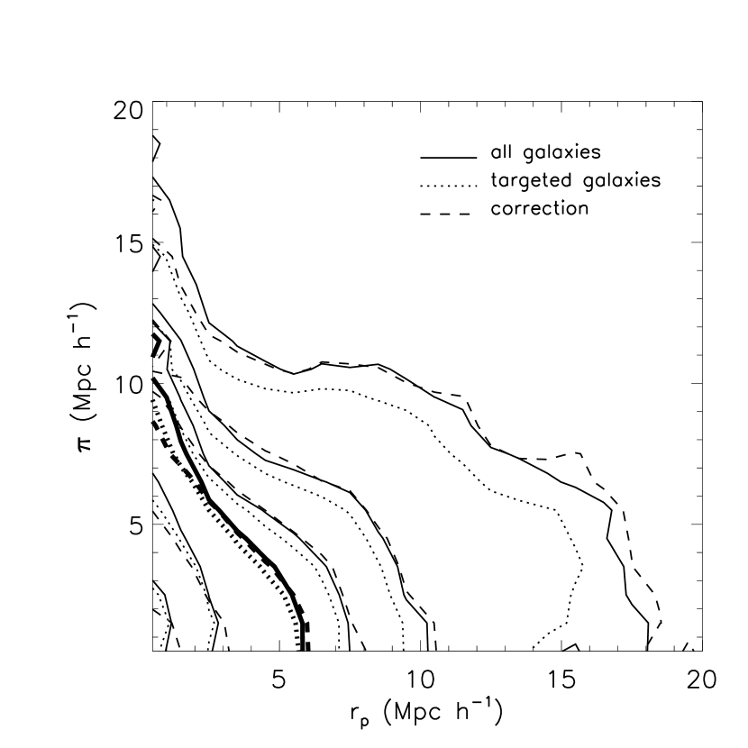
Figure 5: The effects of our target selection algorithm on the two-point correlation amplitude on our GIF mock catalogs. The solid contours show $\xi(r_{p},\pi)$ for all the galaxies in the catalog, with contours levels of 0.25, 0.5, 0.75, 1.0 (bold), 2.0, 5.0. The data have been smoothed with a 3-pixel boxcar in each direction. The dotted contours are for only those galaxies selected to be observed. $\xi(r_{p},\pi)$ of the targeted galaxies underestimates the true correlation amplitude. Dashed contours show a simple correction for untargeted galaxies where the redshift of the nearest neighbor on the sky within the expected photometric redshift error is used for the untargeted galaxy.

A critical function of the GIF mock catalogs is to test the effects of the target-selection algorithm on the measured two-point correlation function. The results are shown in Figure 5. Here we plot the mean two-point correlation amplitude $\xi(r_{p},\pi)$ for all the galaxies in our catalogs in solid contours as well as for only those galaxies selected to be on slitmasks in dotted contours. The correlation amplitude for targeted galaxies alone is lower than for all the galaxies, as expected. We also show in figure 5 the result of a simple correction for this bias. For galaxies not targeted to be on slitmasks, we substitute the redshift of the nearest neighbor on the sky which was targeted and is within the expected photometric redshift error of $z$=0.1 of the un-targeted galaxy and use its redshift as that of the un-targeted galaxy. In this way we use the angular information and the photometric redshift of the un-targeted galaxies and can partially recover the amplitude errors in the correlation analysis.

This correction works extremely well on large scales, $\geq$5 $h^{-1}$ Mpc. The correction underestimates the “finger of god” effect on small scales ($\leq$5 $h^{-1}$ Mpc), where it effectively positions the un-targeted galaxies at the identical physical distances of the nearest neighbors on the sky, thereby reducing the effect of random thermal motion. The conclusion is that the target-selection bias can be corrected in a simple manner on scales $\geq$5 $h^{-1}$ Mpc. The most straightforward means of dealing with the resulting bias on small scales will probably be to filter all models by the same selection procedure, to estimate the degree to which the targeted galaxies are underestimating the correlation amplitude.

3.2 Redshift Distortions in the Measured Two-point Correlation Function

The mock catalogs can be used to quantify the precision with which we can measure redshift distortions in the two-point correlation function $\xi(r_{p},\pi)$ in the DEEP2 survey. Redshift distortions are expected on small scales due to the random internal velocities of galaxies in groups and clusters, creating so-called “fingers of god” on small scales ($\leq$ 5 $h^{-1}$ Mpc). This effect can be seen in the redshift two-point correlation function $\xi(r_{p},\pi)$ shown in figure 4 as the elongation along the y-axis (separation along the line of sight) at small scales. On larger scales a flattening of the two-point correlation function contours can be seen, which is due to coherent infall of galaxies resulting from the gravitational pull of large forming superclusters. A standard method by which to quantify these redshift-space distortions is to measure $\xi_{2}$/$\xi_{0}$, the quadrupole to monopole moments of the two-point correlation function (Hamilton, 1998). The multipole moments of the two-point correlation function are defined as

$$\xi_{l}(s)=(2l+1)/2\int{\xi(r_{p},\pi)P_{l}(\cos\theta)d\cos\theta}.$$ (4)

$\xi_{2}$/$\xi_{0}$ is greater than zero on small scales where the “fingers of god” are apparent and less than zero on large scales where coherent infall appears. Figure 6 plots $\xi_{2}$/$\xi_{0}$ as a function of redshift separation, with 1$\sigma$ errors as derived from the six separate GIF mock catalogs. Unlike the measurement of $\xi(r_{p},\pi)$, the covariance matrix is large only on large scales, greater than 12 $h^{-1}$ Mpc. The bias of our target selection procedure can be seen as the dotted line, and the correction discussed in the last section is shown with a dashed line. As with the $\xi(r_{p},\pi)$ statistic, the effect of target selection is to slightly decease the amplitude of $\xi_{2}$/$\xi_{0}$ on all scales. The applied correction increases $\xi_{2}$/$\xi_{0}$ on scales $\geq$5 h^-1 Mpc and underestimates it on small scales. We will need to apply a bias correction to account for this in the survey. However, the mock catalogs show clearly that the correlation anisotropy will be robustly detected in the DEEP2 survey.

The amount of flattening seen on large scales constrains the parameter $\beta\equiv\frac{\Omega_{m}^{0.6}}{b}$, where $b$ is the bias between the galaxy and dark matter clustering. In linear theory,

$$\xi_{2}/\xi_{0}=f(n)\frac{\frac{4}{3}\beta+\frac{4}{7}\beta^{2}}{1+\frac{2}{3}\beta+\frac{1}{5}\beta^{2}}$$ (5)

where $f(n)$ =(3+$n)/n$ and $n$ is the index of the two-point correlation function in a power-law form: $\xi\propto r^{-(3+n)}$ (Hamilton, 1992). Our 1$\sigma$ errors plotted in figure 6 show that in one of our slices we should be able to measure $\beta$ to within +/– 0.2, so that for our full sample of four slices our error on $\beta$ should be +/– 0.1. In order to extract $\Omega_{m}$ from our measurement of $\beta$ we will need to know the absolute bias of our galaxy sample, which we may be able to determine from our measurements of the three-point correlation function relative to the two-point function (see section 3.4).

3.3 Pairwise and Object-weighted Velocity Dispersion

The pairwise velocity dispersion is a parameter which measures the small-scale thermal motions of galaxies and probes the mass density of the universe. It has been measured to be around 400-500 km s^-1 for various redshift surveys at low-$z$ (e.g. Fisher et al. 1994; Marzke et al. 1995; Jing, Mo, & Börner 1998). In this analysis, we confine our test to a measurement of the pairwise velocity dispersion $\sigma_{12}$ by comparing $\xi(r_{p},\pi)$ in real and redshift space on the scale of $r_{p}$=1 $h^{-1}$ Mpc, where the “finger of god” effect dominates redshift distortions. (In this section we will use a subscript R to indicate real space.) For this analysis we use the flux-limited mock catalog before slit selection, averaged over all 6 catalogs.

Following Fisher et al. (1994), we first define

$$\xi(r_{p}=1,\pi)\equiv 0.5[\xi(r_{p}=0.5\>\mathrm{Mpc}\,h^{-1},\pi)+\xi(r_{p}=1.5\>\mathrm{Mpc}\,h^{-1},\pi)]$$ (6)

in both real and redshift space, $\xi_{R}(r_{p}=1,\pi)$ and $\xi(r_{p}=1,\pi)$, for values of $\pi\leq$ 20 $h^{-1}$ Mpc. We then normalize $\xi(r_{p}=1,\pi)$ so that our subsequent fitting will be sensitive to the overall shape of $\xi(r_{p}=1,\pi)$ but insensitive to the amplitude:

$$\xi(\pi)=\frac{\xi(r_{p}=1,\pi)}{\int_{0}^{\pi_{max}}\xi(r_{p}=1,\pi)\,d\pi}$$ (7)

where $\pi_{max}$ is the maximum value of $\pi$ used in the analysis (here $\pi_{max}$=20 $h^{-1}$ Mpc).

Within the mock catalogs, the pair-weighted dispersion of the known peculiar velocities is 500 km s^-1 for galaxies with radial separations $\leq$20 $h^{-1}$ Mpc within a projected distance of 1 $h^{-1}$ Mpc, as measured in real space. The mean infall velocity, $v_{12}$, is 160 km s^-1 at the same scale. To determine $\sigma_{12}$ in the redshift space catalog, we construct models of $\xi(\pi)$ by convolving the measured $\xi_{R}(\pi)$ in real space with different distribution functions of velocity differences for pairs of galaxies separated by vector distance $\mathbf{r}$ to compare with the measured $\xi(\pi)$. Let the vector $\mathbf{r}$ separating two galaxies be decomposed into a transverse component $r_{p}$ and a line-of-sight component $y$, where $y$ can be converted into a velocity separation at the given redshift. Then the velocity difference is given as $\pi$-$y$, and the convolution becomes

$$1+\xi(\pi)=\frac{1}{\sqrt{2}}\int\frac{dy}{\sigma_{12}}\>(1+\xi_{R}(\pi))\>exp(-\sqrt{2}\left|\frac{\pi-y-yv_{12}(r)/r}{\sigma_{12}}\right|),$$ (8)

where $r^{2}=r_{p}^{2}+y^{2}$. For the mean infall velocity, $v_{12}(r)$, we use the similiarity solution of Davis & Peebles (1983), $v_{12}\sim r/[1+(r/r_{0})^{2}]$ with $r_{0}$=5.83 h^-1 Mpc. At $z$=1 in a LCDM model this corresponds to 71 km s^-1. Figure 7 plots the measured $\xi(\pi)$ with models of $\sigma_{12}$ equal to 350, 400, and 450 km s^-1. Using a minimum chi-squared test, we find that the best fit is $\sigma_{12}$=410 km s^-1 with a 1$\sigma$ error of 80 km s^-1. If we instead use a mean infall velocity of $v_{12}(r)$=160 km s^-1 at $r$=1 $h^{-1}$ Mpc, we find $\sigma_{12}$=485 km s^-1, consistent with the measured peculiar velocity dispersion in the mock catalog of 492 km/s. Note that redshift space distortions are larger at high redshift than at low redshift by the factor $(1+z)$, and that we have removed this extra factor in our modeling of $\sigma_{12}$ by simply using 1+$z$=2.

The $\sigma_{12}$ statistic is known to be unstable, however, as it is pair-weighted and therefore quite sensitive to rare, rich galaxy clusters (Davis, Miller, & White, 1997). Jing & Börner (1998) also argue that the measured value of $\sigma_{12}$ depends strongly on the assumed value of $v_{12}$, the mean infall velocity, which here we have modeled in an adhoc manner. We therefore also measure the galaxy-weighted velocity dispersion $\sigma_{1}$, which is a more stable statistic and a measure of the one-dimensional peculiar velocity dispersion of galaxies relative to their neighbors. This statistic is more easily evaluated and does not rely on assumed values of the mean infall. Following the prescription of Baker, Davis, and Lin (2000) we construct the velocity distribution $D(\Delta v)$ by a weighted sum over $N_{g}$ galaxies:

$$D(\Delta v)=\frac{1}{N_{g}}\sum_{i=1}^{N_{g}}w_{i}\left[P_{i}(\Delta v)-B_{i}(\Delta v)\right]$$ (9)

where $w_{i}$ is the weight for each galaxy, determined by the number of neighbors in excess of a random background. Here $P_{i}(\Delta v)$ is the distribution of neighboring galaxies within a cylinder of projected radius $r_{p}$ and half-length $v_{l}$ in redshift space, while $B_{i}(\Delta v)$ is the background distribution expected for an unclustered galaxy distribution. Baker et al. (2000) describe a weighting scheme where galaxies for which the distribution is negative can be incorporated into $D(\Delta v)$ by considering the high and low density samples separately and combining them, weighting by the number of objects included in each sample. This statistic results in an unbiased, object-weighted measure of the thermal energy of the galaxy distribution. The velocity distribution $D(\Delta v)$ can be seen in figure 8. To measure the intrinsic dispersion, $\sigma_{1}$, we model the real space correlation function $\xi(r)$ convolved with an exponential velocity broadening function,

$$f(v)=\frac{1}{\sigma_{1}}exp(-\frac{|v|}{\sigma_{1}})$$ (10)

(see Davis, Miller, & White (1997) and Baker et al. (2000) for details). We measure $\sigma_{1}$=180 +/–20 km s^-1 for a $r_{p}=1$ $h^{-1}$ Mpc and $v_{l}=$2500 km s^-1. We find similar results for $r_{p}=$2 $h^{-1}$ Mpc. The model fit for $\sigma_{1}$=180 km s^-1 is shown in figure 8.

This value of $\sigma_{1}$ should be compared to the 1-D rms peculiar motion of 315 km s^-1 for the GIF mock galaxies in the catalog. This rms peculiar motion includes large scale flows, while $\sigma_{1}$ measures only the nonlinear thermal component of the peculiar velocities. The difference is of the magnitude expected. Note that Baker et al. (2000) measured $\sigma_{1}=126\pm 10$ km s^-1 for the LCRS survey, and it is quite likely that DEEP2 will report a value lower than this for the distant Universe. This might become a modest mismatch between the GIF simulations and reality.

3.4 The Three-point Correlation Function

The highly non-Gaussian nature of the galaxy distribution can be described with the hierarchy of $N$-point correlation functions. In particular, the three-point correlation function contains a wealth of information on gravitational collapse, initial conditions of the power spectrum, and most importantly, bias and galaxy formation. In this paper we present preliminary measurements of the three-point correlation function in our DEEP2 GIF mock galaxy catalogs. Our goal is to show that the three-point correlation function can be measured with sufficient accuracy to be interesting and that the our selection procedure does not systematically bias our results to a degree that would hinder proper interpretation.

The three-point correlation function is defined as the reduced joint probability of finding a triplet of galaxy at a particular configuration (Peebles, 1980). We have used the estimator by Szapudi & Szalay (1998) for extracting the three-point function:

$$\zeta=(DDD-3DDR+3DRR-RRR)/RRR.$$ (11)

In this equation contributions to a triplet from the data and a random set are denoted with a $D$ and $R$ respectively. The above estimator is expected to be the most accurate edge-corrected formula in the family of estimators based on triplets.

For our measurements of the GIF mock catalogs we chose eight logarithmic bins centered on 0.613 $h^{-1}$ Mpc to 10.779 $h^{-1}$ Mpc. All possible triangles with those sides (allowed by the triangle inequality) were used, i.e. 76 measurements were performed for each sample. The fast $N$-point correlation code by Moore et al. (2000) based on a novel double tree algorithm was used for the calculations.

We have divided the GIF mock galaxy catalogs into four redshift ranges $z$=0.7–0.9, 0.9–1.1, 1.1–1.3, and 1.3–1.5. For each redshift range, we used the six independent catalogs to enable a calculation of the cosmic (co)variances. Finally, for each simulation we calculated the three-point correlation function for all the galaxies in the catalog, as well as for only those galaxies which would be selected to be observed using our target selection slitmask algorithm. We used four times as many random points as galaxies for our measurements.

Figure 9 contains the binned results for the shallowest slice, $z$=0.7–0.9. For this preliminary investigation the results are interpreted in terms of the simple hierarchical assumption (Davis & Peebles, 1983; Peebles, 1980),

$$\zeta=Q_{3}\left(\xi_{1}\xi_{2}+\xi_{2}\xi_{3}+\xi_{3}\xi_{1}\right).$$ (12)

The three-point function is plotted in terms of the hierarchical term on the right. If this equation were exact the result would be a straight line, as illustrated with a dotted line for the case $Q_{3}=1$. Note that $Q_{3}$ shows a weak scale dependence.

According to figure 9, the hierarchical assumption gives a good qualitative description of the data. The tight relation illustrates the quality obtainable by the DEEP2 redshift survey. The scatter is due to measurement errors, cosmic variance, and an intrinsic shape dependence of the three-point correlation function with scale. The increasing error bars on large scales is inevitable because of cosmic variance. With a cross-scan size of 20 $h^{-1}$ Mpc, triangles with baselines $>$10 $h^{-1}$ Mpc will be poorly contrained by the DEEP2 survey. Figure 9 shows that the effect of the target selection bias is to decrease $\zeta$ by $\sim$20%. This, of course, will have to be carefully modelled in analyses of the real data.

Quantifying and separating the intrinsic shape dependence of the $\zeta$ with scale is the key to determining bias from the three-point correlation function. Analysis on quasilinear scales (Fry, 1994) suggests that $\zeta$ can be used for a determination of the galaxy bias that is independent from studies of kinematics or redshift-space distortions. In this way we will hopefully be able to measure absolute biases instead of relative biases. This is left for a subsequent paper; here our purpose is mainly to illustrate the feasibility of a high accuracy three-point measurement with the DEEP2 redshift survey, and to show that the incompleteness caused by the slitmask algorithm does not cause significant, uncontrollable systematic errors.

3.5 Measuring $\sigma_{8}$ and Relative Galaxy Bias as a Function of Redshift

We expect to measure the evolution of $\sigma_{8}$ as a function of redshift for the galaxies observed in the DEEP2 survey. As a simple test of the sensitivity of this measure, we use a counts-in-cells analysis to calculate $\sigma_{8}$ in both our Hubble Volume and GIF simulations mock galaxy catalogs in redshift bins of $\Delta z$=0.1. The counts-in-cells method (Peebles, 1980) uses the moments of the counts of numbers of galaxies in spheres of a given size to quantify the amount of galaxy clustering present.

By counting objects in randomly-placed spherical cells ($N_{i}$) of radius $l$, one can determine the moments of the counts:

$$\mu_{1}=<N_{i}>$$ (13)

$$\mu_{2}=<(N_{i}-<N_{i}>)^{2}>$$ (14)

For each mock catalog, we created 40,000 spherical cells with radii of 8 Mpc $h^{-1}$ and randomly placed them throughout the catalog, ensuring that the centers of the cells were at least 8 $h^{-1}$ Mpc away from the boundary of the mock catalog. In this way none of the cells overlapped the catalog boundaries. We then divided the mock catalog into slices of $\Delta z$=0.1 bins (eg. $z$=0.7–0.8) and calculated the moments of the galaxy counts and $\sigma_{8}$ as a function of redshift. These moments are related to the volume-integrated two-point correlation function and $\sigma_{8}$ as:

$$\mu_{2}=\mu_{1}+\mu_{1}^{2}\overline{\xi_{2}}$$ (15)

$$\sigma_{l}=\sqrt{\overline{\xi_{2}}}.$$ (16)

We performed this analysis on both the Hubble Volume and GIF mock catalogs, as each has an emphasis on different properties which will be relevant in our DEEP2 survey data. The GIF mock catalogs do not have continuous evolution as they are made from three snapshot outputs at different redshifts stacked in $z$-space. However, we were able to use the absolute magnitudes of the galaxies to apply a realistic magnitude-limited selection function, and as a consequence the galaxies at high-$z$ are intrinsically more luminous than those at low-$z$. Since bias is expected to be luminosity-dependent, the inherent bias of the galaxies in the GIF catalogs will change with redshift. The Hubble Volume catalogs, however, have realistic continuous evolution in their light-cone output, but the bias should change more slowly with redshift as the galaxy selection is the same at all redshifts.

To take into account the changing selection function with redshift, for the GIF mock catalogs we created a volume-limited sample within each redshift bin. We used the absolute $B$-band magnitude to keep only those galaxies which are bright enough so that they could have been observed at the far end of the redshift bin. For the Hubble Volume mock catalogs we did not have magnitudes and so were not able to create volume-limited samples. The Hubble Volume simulations therefore have a slight density gradient within each redshift bin. We tested the effects of this small density gradient on the counts-in-cells results from the GIF mock catalogs with and without volume-limited samples and found a 1$\%$ difference in the values of $\sigma_{8}$ in the volume-limited sample, and therefore conclude that it is a negligible effect.

The results for the Hubble Volume mock galaxy catalogs are shown in figure 10a. The solid line is the mean $\sigma_{8}$ as measured in our sixteen independent mock catalogs, while 1$\sigma$ errors as determined from the variance between the different catalogs are shown in dashed lines. The expected linear evolution of $\sigma_{8}$ in the underlying dark matter is shown as a dash-dot line (normalized to 0.9 at $z$=0, as were the simulations; see Fry 1996 for analytic formula). If we fit our estimates of $\sigma_{8}(z)$ of the galaxies to the analytical form

$$\sigma_{8}(z)=A\left(\frac{1+z}{2}\right)^{\alpha}$$ (17)

we find A=0.64 (1$\sigma$=0.01) and $\alpha$=–0.51 (0.10). The covariance between A and $\alpha$ is low; the off-diagonal elements of the covariance matrix are equal to -0.36.

An evolution of the bias between the galaxies and the dark matter is apparent in the shallower slope of the galaxy clustering evolution compared to the dark matter linear evolution prediction. Figure 10b is a plot of the estimated bias, equal to $\sigma_{8}$(galaxies)/$\sigma_{8}$(dark matter). The bias is slightly larger at high-$z$, as is expected from hierarchical structure formation models. An analytic fit to the slope of the bias evolution results in a best fit of A=1.16 (1$\sigma$=0.01) and $\alpha$=0.37 (0.10), with the same low covariance as the $\sigma_{8}$ analysis. Evolution of bias is therefore expected to be present at the 4$\sigma$ level within a single slice of the DEEP2 survey, but separation of the changing bias from the evolving matter distribution will be complex. For a given cosmological model, we can use linear theory to calculate the latter quantity.

The evolution of $\sigma_{8}$ for the GIF mock catalogs is shown in figure 11. The best fit to the analytic form for the evolution of $\sigma_{8}$ is A=0.80 (0.01) and $\alpha$=0.38 (0.13). The change of bias with redshift is best fit by A=1.45 (0.01) and $\alpha$=1.26 (0.13). Here we are using mock galaxies of all luminosities, so that the bias changes with redshift not primarily because of evolution but because at high-$z$ we measure only the intrinsically more luminous galaxies in our magnitude-limited sample, and these objects are more clustered at all redshifts. This is an effect we will see in the DEEP2 survey, where we will have to subdivide the galaxies by linewidths or luminosity to separate the effects of bias evolution from differing bias in different galaxy populations.

In figure 12 we show the B-band luminosity function (LF) of one GIF mock catalog in different redshift bins. At lower redshifts, the LF extends to galaxies with absolute B mag of -19, but at higher redshifts only the brightest galaxies are seen. This change of the LF with redshift is primarily due to our apparent magnitude sample selection, though there is some inherent evolution in the LF which is included in the GIF simulations. We made subsamples of the galaxy catalogs based on absolute B-band magnitude and show the bias evolution for different magnitude ranges in figure 13. There is a clear trend between galaxy magnitude and the amplitude as well as evolution of bias. The brighter galaxies have a higher bias as well as stronger evolution. The values of the amplitude of the bias at $z$=1 (A) and the slope of the evolution ($\alpha$) are given in the figure, with 1$\sigma$ errors in parentheses. We are able to measure relative bias between galaxy types to within 0.02 and measure evolution of bias at the 5-6$\sigma$ level for the brightest galaxies (–24$<$B mag$<$–21) and at the 3-4$\sigma$ level for the fainter galaxies (–21$<$B mag$<$–19). Note that these values for the bias are calculated in redshift space.

4 DISCUSSION

A key goal of the DEEP2 redshift survey of galaxies is to constrain the evolution of large-scale structure in the universe. In most cosmological models, the galaxy distribution is expected to evolve measurably between $z=0$ and $z=1$, and different types of galaxies are expected to evolve independently. The survey will hopefully be sufficiently robust to allow subdivision of the sample so as to separately constrain the evolving bias of distinct classes of galaxies. As indicated by the modest size of the error bars in the comparison of mock catalogs, clustering constraints derived from the DEEP2 survey are expected to have only modest cosmic variance. They will thus supersede the current contradictory constraints on the strength of high redshift galaxy clustering derived from the modest surveys undertaken to date. As shown in figure 4, each slice of the DEEP2 survey should lead to a 10% estimate of the correlation length of clustering $r_{0}$. Subdivision into differing samples will not degrade the measurement precision as rapidly as $n^{-1/2}$, because cosmic variance is dominant in this estimate, not Poisson noise.

The tests described above demonstrate the power of the DEEP2 survey for refined estimates of redshift space distortions in the distant Universe. The high resolution of the DEIMOS spectra will yield high quality redshifts, thus enabling the study of the kinematics internal to the galaxies and the kinematics of small scale clustering at $z=1$. It should be readily possible to measure all these quantities within the survey volume, although the estimated $\sigma_{12}$ is likely to be too noisy to set useful constraints. We note that $\sigma_{1}$ is measureable to 10% precision, while $\sigma_{12}$, after averaging over all 6 mock slices, is measurable to only 20% precision. The Kaiser infall effect on large scales should yield a 10% measurement of $\beta$, when averaging over the full survey. Estimates of the infall from subsamples of the DEEP2 survey will not degrade as rapidly as the Poisson noise, since this statistic is also dominated by cosmic variance.

Precise constraints on the evolution of galaxy correlations will not only greatly improve our understanding of galaxy formation in hierarchical models, they will also facilitate novel cosmological tests of considerable interest. For example, the counting of galaxies in the classic $dN/dz$ test (Newman & Davis, 2000; 2001) is capable of setting good constraints on cosmological parameters such as $w\equiv P/\rho$ versus $\Omega_{m}$, but serious degeneracy will remain even after counting $10^{4}$ galaxies in the range $0.7<z<1.5$. The magnitude-redshift relation derived from distant supernovae leads to constraints with very similar degeneracy between $w$ and $\Omega_{m}$. To a considerable degree this degeneracy can be broken by additional, complementary tests. For example, the expected ratio of the $J_{3}$ integral of $\xi(r)$ at $z=1$ compared to that at $z=0$ has a different dependency on these same cosmological parameters, leading to contours of constant $J_{3}$ ratio that cross those of the $dN/dz$ test. Further tests, such as the abundance of clusters of galaxies, lead to quite different constraints in this same parameter space plane (Newman et al. 2001). Simultaneous execution of all these tests with the DEEP2 survey data is thus capable of setting rather tight constraints on $w$ and $\Omega_{m}$.

5 CONCLUSIONS

The clustering of galaxies at high redshift is intimately connected to our incomplete understanding of galaxy formation, and both disciplines will advance as we analyze the details of clustering in the soon-to-begin DEEP2 survey. In order to study the precision with which one can expect to measure the clustering of galaxies at $z\sim 1$, we have generated a series of mock catalogs of the DEEP2 galaxy redshift survey. The mock catalogs are derived from two separate VIRGO simulations, one with continuous evolution of the underlying structure but inadequate mass resolution, and another with adequate mass resolution but which required the stacking of numerous simulation volumes to achieve a size sufficient to match the redshift range of the survey.

The DEEP2 survey will use multislits, rather than multifibers, to multiplex spectroscopic targets. The necessity of avoiding overlapping spectra in the survey limits the sampling efficiency of spectroscopic target selection, especially in regions of the sky with higher than average surface density of galaxies. The tentative selection algorithm for the survey will lead to $\sim$ 70$\%$ success rate in target selection. Although the resulting bias substantially affects the angular correlations of the selected targets, the correlations observed in redshift space are only modestly affected, and the bias can be largely removed by double counting galaxies closest on the sky and within the photometric redshift error to those galaxies not selected for spectroscopy.

Distortions in redshift space as measured by the $\xi(r_{p},\pi)$ diagram will be cleanly detected in the DEEP2 survey, and we expect to measure both the ”fingers of god” on small scales and coherent infall motions of galaxies on large scales. Additional tests of velocity field effects, such as the $\sigma_{1}$ test of Davis, Miller, & White (1997), will be readily possible with the sample and will be much less affected by the bias in the target selection algorithm.

We expect to be able to measure $\sigma_{8}$ to within 10% in individual slices of the survey. Assuming a cosmological model, we can detect the evolution of relative bias with 4–5$\sigma$ significance within the volume of the DEEP2 survey itself, with more precise measurements for the brightest subsample of galaxies.

The survey geometry is designed to allow a good measure of the three-point clustering amplitude for scales $r\leq 10h^{-1}$ Mpc, and tests of the mock catalogs indicate that this will indeed be possible. Such a measure will allow an independent test of the bias in the galaxy distribution.

The DEEP2 survey is designed to be a comprehensive study of the Universe at $z=1$. Having a sample of high redshift galaxies comparable in quality to those available locally will enable many independent tests of the evolution of structure in the Universe. With numerous cross checks and subdivision of the redshift catalogs into different classes of galaxies, we should be able to untangle evolution in the galaxy bias from evolution in the underlying matter distribution.

We would like to thank Guinevere Kauffmann for graciously allowing us to use her semi-analytic GIF simulations. IS would like to thank his collaborators on npt (the fast $N$-point code), especially Andrew Connolly, Bob Nichol, Andrew Moore, and Alex Szalay, for their help. We acknowledge helpful discussions with Jeff Newman. This project was supported by the NSF grant AST-0071048. A.L.C. would like to acknowledge an NSF Graduate Research Fellowship. IS was partially supported by a NASA AISR, NAG-10750. We also acknowledge the support of Sun Microsystems.

Figure 1: One of our mock galaxy catalogs constructed from the Virgo Consortium Hubble Volume simulations, shown in both real and redshift space. This lightcone output has the advantage of continuous evolution, but the mass resolution is poor.

Figure 2: $a$. The redshift selection function which was applied to the Hubble Volume mock catalogs. $b$. A histogram of the redshift distribution of galaxies in one of the Hubble Volume mock catalogs.

Figure 3: One of our GIF mock galaxy catalogs shown in redshift space. In the top panel are all the galaxies in this mock catalog, while only those targeted for slitmasks are shown in the middle panel. The galaxies for which we would not obtain spectra are in the lower panel. This simulation has better mass resolution than the Hubble Volume simulation and has semi-analytic models applied. We used the known absolute luminosity of each galaxy to create a flux-limited sample of $I$=23.4 mag.

Figure 4: The mean redshift-space two-point correlation function $\xi(r_{p},\pi)$ of our six GIF mock galaxy catalogs is shown in solid lines, with 1$\sigma$ errors in dotted lines. The data have been smoothed with a 3-pixel boxcar in each direction. The contour levels are 0.25, 0.5, 0.75, 1.0 (bold contour), 2.0, and 5.0. The scale length of the clustering is $\sim$ 6 $h^{-1}$ Mpc, as seen on the x-axis.

Figure 6: Redshift distortions seen in the two-point correlation function are quantified by the quadrupole-to-monopole ratio $\xi_{2}$/$\xi_{0}$ of $\xi(r_{p},\pi)$, plotted for all the galaxies in the mock catalogs as a solid line with 1$\sigma$ errors. The dash-dot line is for only those galaxies selected to be observed on slitmasks, and the dashed line show the results of a simple correction for untargeted galaxies. Dotted lines show models of $\xi_{2}$/$\xi_{0}$ for different values of $\beta$.

Figure 7: Measured $\xi(\pi)$ in redshift space compared to models with different pairwise velocity dispersions. The best fit is $\sigma_{12}$=410 +/–80 km s^-1.

Figure 8: Galaxy-weighted velocity distribution $D(\Delta v)$ for the six GIF mock catalogs. The best fit model shown has $\sigma_{1}$=180 km s^-1.

Figure 9: The three-point correlation function as a function of the hierarchical term $\xi_{1}\xi_{2}+\xi_{2}\xi_{3}+\xi_{3}\xi_{1}$ in the redshift range $z$=0.7–0.9. The open squares display the measurements for all the galaxies in the mock catalogs, while the solid squares show measurements for only those galaxies targeted by the 2-pass slitmask algorithm. The data were binned in terms of the heirarchical term, and the errorbars correspond to the dispersion of the six mock catalogs as well as scatter within the bin from one catalog. The error bars on the solid squares are comparable to those displayed but are not shown for clarity. The dotted line corresponds to a simple hierarchical model with $Q_{3}=1$.

Figure 10: a. The mean evolution of $\sigma_{8}$ as measured for galaxies in the Hubble Volume mock catalogs. 1$\sigma$ errors are plotted in dashed lines. The dash-dot line shows the expected linear evolution of $\sigma_{8}$ of the underlying dark matter distribution, normalized to $\sigma_{8}$ of 0.9 at $z$=0. b. The mean evolution of bias as defined by $\sigma_{8}$(galaxies)/$\sigma_{8}$(dark matter). A fit of bias=$A\left(\frac{1+z}{2}\right)^{\alpha}$ results in an amplitude $A$=1.16 and slope $\alpha$=0.37.

Figure 11: a. The mean evolution of $\sigma_{8}$ as measured for galaxies in the GIF simulation mock catalogs. b. The change of bias with redshift. Here the increase of bias at high-$z$ is not solely the result of evolution, as the galaxies at high-$z$ in our sample are more luminous and therefore have a higher degree of bias on the whole.

Figure 12: The B-band luminosity function (LF) of one of our GIF mock catalogs in different redshift bins. The difference in the LF as a function of redshift is due mainly to the selection effects of our apparent magnitude-limited sample, though there is some intrinsic evolution of the LF present in the simulations.

Figure 13: Bias evolution for subsamples of the GIF mock catalogs selected by B-band magnitude. Here the change in bias with redshift is due to evolution within a specific galaxy type. The brightest galaxies are seen to have a larger bias and stronger evolution with $z$.

References

- Baker et al. (2000) Baker, J. E., Davis, M., & Lin, H. 2000,ApJ, 536, 112
- Cowley et al. (1997) Cowley, D. J., Faber, S., Hilyard, D. F., James, E., & Osborne, J. 1997, SPIE, 2871, 1107
- Davis & Peebles (1983) Davis, M. & Peebles, P. J. E. 1983, ApJ, 267, 465
- Davis, Miller, & White (1997) Davis, M., Miller, A., & White, S. D. M. 1997, ApJ, 490, 63
- Davis et al. (2000) Davis, M., Newman, J. A., Faber, S. M., & Phillips, A. C. 2000, Proceedings of the ESO/ECF/STSCI Workshop on Deep Fields, Garching Oct 2000, (Publ: Springer)
- Evrard et al. (2000) Evrard, A. E., MacFarland, T., Couchman, H. M. P., Colberg, J. M., Yoshida, N., White, S. D. M., Jenkins, A., Frenk, C. S., Pearce, F. R., Efstathiou, G., Peacock, J. A., & Thomas, P. A. 2000, in preparation
- Fisher et al. (1994) Fisher, K. B., Davis, M. Strauss, M. A., Yahil, A.,& Huchra, J. P. 1994, MNRAS, 267, 927
- Fry (1996) Fry, J. N. 1996, ApJ, 461, L65
- Fry (1994) Fry, J. N. 1994, Phys. Rev. Lett. 73, 215
- Giavalisco et al. (1998) Giavalisco, M., Steidel, C. C., Adelberger, K. L., Dickinson, M., Pettini, M., & Kellogg, M. 1998, ApJ, 503, 543
- Hamilton (1992) Hamilton, A. J. S. 1992, ApJ, 385, L5
- Hamilton (1998) Hamilton, A. J. S. 1998, ASSL Vol. 231: The Evolving Universe, 185
- Jenkins et al. (1998) Jenkins, A., Frenk, C. S., Pearce, F. R., Thomas, P. A., Colberg, J. M., White, S. D. M., Couchman, H. M. P., Peacock, J. A., Efstathiou, G., Nelson, A. H. 1998, ApJ, 499, 20
- Jing, Mo, & Börner (1998) Jing, Y. P., Mo, H. J., & Börner, G. 1998, ApJ, 494, 1
- Jing & Börner (1998) Jing, Y. P. & Börner, G. 1998, ApJ, 503, 502
- Kauffmann et al. (1999) Kauffmann, G., Colberg, J. M., Diaferio, A., White, S. D. M. 1999, MNRAS, 303, 188
- Marzke et al. (1995) Marzke, R. O., Geller, M. J., da Costa, L. N., Huchra, J. P. 1995, AJ, 110, 477
- Moore et al. (2000) Moore, A., et al. To appear in Proceedings of MPA/MPE/ESO Conference ”Mining the Sky”, July 31 - August 4, 2000, Garching, Germany. astro-ph/0012333
- Newman & Davis (2000) Newman, J. & Davis, M. 2000, ApJ, 534, 11
- Newman & Davis (2001) Newman, J. & Davis, M. 2001, in preparation
- Peebles (1980) Peebles, P. J. E. 1980, The Large-Scale Structure of the Universe (Princeton Univ. Press)
- Postman et al. (1998) Postman, M., Lauer, T. R., Szapudi, I., & Oegerle, W. 1998, ApJ, 506, 33
- Scoccimarro et al. (1998) Scocciamarro, R., Colombi, S., Fry, J., Frieman, J., Hivon, E., & Melott, A. 1998, ApJ, 496, 586
- Szapudi & Szalay (1998) Szapudi, I. & Szalay, A. S. 1998, ApJ, 494, L41
- White, Davis, Efstathiou, & Frenk (1987) White, S. D. M., Davis, M., Efstathiou, G., & Frenk, C. 1987, Nature, 330, 451
- Wilson et al. (2000) Wilson, G., Kaiser, N., Luppino, G. A., & Cowie, L. L. 2000, preprint astro-ph/0008504
- Wechsler et al. (1998) Wechsler, R., Gross, M., Primack, J., Blumenthal, G., & Dekel, A. 1998, ApJ, 506, 19
- Yoshida et al. (2000) Yoshida, N., Colberg, J. M., White, S. D. M., Evrard, A. E., MacFarland, T., Couchman, H. M. P., Jenkins, A., Frenk, C. S., Pearce, F. R., Efstathiou, G., Peacock, J. A., & Thomas, P. A. 2000, submitted to MNRAS