Relativistic Beaming and Flux Variability in
Active Galactic Nuclei

Abstract

We discuss the impact of special relativistic effects on the observed light curves and variability duty cycles of radio-loud active galactic nuclei (AGNs). We model the properties of AGN light curves at radio wavelengths using a simulated shot noise process in which the occurrence of major flaring events in a relativistic jet is governed by Poisson statistics. We show that flaring sources whose radiation is highly beamed toward us are able to reach very high flux levels, but will in fact spend most of their time in relatively low flaring states. This is primarily due to relativistic Doppler contraction of flaring time scales in the observer frame. The fact that highly beamed AGNs are not observed to return to a steady-state quiescent level between flares implies that their weakly beamed counterparts should have highly stable flux densities that result from a superposition of many long-term, low-amplitude flares. The “apparent” quiescent flux levels of these weakly beamed AGNs (identified in many unified models as radio galaxies) will be significantly higher than their ”true” quiescent (i.e., non-flaring) flux levels. We have also performed Monte Carlo simulations to examine how relativistic beaming and source variability bias the selection statistics of flat-spectrum AGN samples. We find that in the case of the Caltech-Jodrell Flat-spectrum survey (CJ-F), the predicted orientation bias towards jets seen end-on is weakened if the parent population is variable, since the highly beamed sources have a stronger tendency to be found in low flaring states. This effect is small, however, due to the fact that highly beamed sources are relatively rare, and in most cases their flux densities will be boosted sufficiently above the survey limit such that they will be selected regardless of their flaring level. We find that for larger flat-spectrum AGN surveys with fainter flux density cutoffs, variability should not be an appreciable source of selection bias.

1 Introduction

One of the hallmarks of flat-spectrum radio-loud active galactic nuclei (AGNs) is their tendency to display large flux density variations over a wide range of wavelengths. Studies of complete AGN samples (e.g., Aller et al. 1992; Lähteenmäki & Valtaoja 1999; Lister et al. 2001) have shown that the degree of variability at radio wavelengths is well-correlated with the prominence of a bright, flat-spectrum core component that is thought to harbor the supermassive black hole and accretion disk that power the AGN. Parsec-scale images made with VLBI techniques show that this core is usually located at the base of a highly collimated, relativistic outflow.

The extremely high speeds of AGN jets are responsible for numerous biases in the observed properties of samples selected on the basis of core flux density, due to special relativistic effects (e.g., Scheuer & Readhead 1979). For example, the distribution of source orientations in such samples will be heavily weighted towards jets seen nearly end-on, due to relativistic beaming of radiation in the direction of motion. These highly beamed sources (also known as blazars) will also tend to have more variable light curves than typical radio-loud AGNs, since any intrinsic flux variations associated with the relativistic outflow will have their timescales shortened and amplitudes boosted in the observer’s frame.

Previous theoretical studies of observational biases associated with relativistic beaming in AGNs (e.g., Vermeulen & Cohen 1994; Lister & Marscher 1997) have considered only steady-state fluxes, and have not taken into account possible additional biases due to variability. In most flux-limited samples of astronomical objects, source variability is not usually a major source of bias, since its effects tend to be statistically averaged out in the sampling process. The situation is different, however, for samples of objects whose flux densities are relativistically beamed, such as flat-spectrum AGNs and gamma-ray bursts. As we will show in this paper, the observed variability duty cycles of these objects (i.e., the fraction of time spent above a particular flux level) can be strongly affected by beaming, and should therefore be considered as a possible source of bias in flux-limited samples. Since these types of samples are often used to infer general properties of the parent population, it is important to ascertain the strength of this effect.

In the first part of this paper we develop a simple shot-noise variability model to examine the effects of relativistic beaming on the radio light curves and duty cycles of AGNs. We describe the parameters of our model in § 2, and compare our simulations to observed AGN light curves in § 3. In § 4 we show how highly beamed AGNs are able to reach very high flux levels, but will in fact be observed to spend most of their time in low flaring states. In the remaining portion of the paper we use Monte Carlo simulations to model the beaming and variability properties of the blazar parent population, and determine the degree to which core-selected AGN samples are additionally biased by source variability. In § 5 we show that despite the dramatic range of observed variability levels in blazars, their overall parent population likely consists of weakly beamed sources with stable flux levels that arise from the superposition of many long-term flares. We find that as a result, the “quiescent” flux levels of these sources (identified in most unified models as radio galaxies) are significantly higher than their “true” quiescent (i.e., non-flaring) levels. We further demonstrate how the predicted orientation bias in medium-sized, flat-spectrum AGN samples is slightly weakened in the case of a flaring source population. We summarize our main findings in § 6.

Throughout this paper we use a Freidmann cosmology with zero cosmological constant, $q_{o}=0.1$, and a Hubble constant $h=0.65$ measured in units of $100\rm\;km\;s^{-1}\;Mpc^{-1}$. Over the redshift range of our simulations, this choice of cosmology gives luminosity distances that are within $\sim 10$% of those calculated using more contemporary $\Omega_{m}=0.28$, $\Omega_{\Lambda}=0.72$ models (e.g., Perlmutter et al. 1999).

2 Variability Model

The study of variability in blazars at radio wavelengths is hindered by complications arising from relativistic beaming. The true jet speeds and orientations of individual objects are in most cases poorly known, which makes it difficult to disentangle possible beaming effects from their observed light curves. As a result, there are relatively few observational constraints on the intrinsic amplitudes and timescales of individual flares that are responsible for the majority of flux density variations in radio-loud AGNs.

These considerations have led us to develop a relatively simple stochastic variability model for this study that contains a minimal number of free parameters, yet still reproduces the major variability characteristics of AGNs at radio wavelengths. In this section we describe the parameters of this model, which we will use to create simulated light curves for AGNs having various jet speeds and orientations.

2.1 Rate of flare occurrence

Long-term flux monitoring studies at cm- and mm-wavelengths at the U. Michigan (Hughes et al., 1992) and Metsähovi (Valtaoja et al., 1992) observatories have shown that the flux density variations of AGNs tend to be stochastic (i.e., there are very few instances of periodicity). Rather than being completely random, however, AGN light curves display a flare-like behavior whose spectral properties are consistent with a shot-noise process (Cruise & Dodds, 1985; Hughes et al., 1992; Hufnagel & Bregman, 1992). One way to reproduce shot noise is through a superposition of a series of identical impulses, occurring at intervals dictated by Poisson statistics. In a Poisson process, the overall rate of events is statistically constant, yet the starting times of individual events are independent of all previous ones. The time intervals between events follow an exponential distribution. We will use such a process in our AGN variability model, by assuming a constant flare rate $\rho$, such that the probability that a second flare will occur within a time interval $\tau$ after the first one is $p(\tau)=1-\exp{(-\rho\tau)}$.

Long-term monitoring of bright AGNs in the mm-wave regime at the Metsähovi radio observatory has shown that on average, most sources experience one major flare per year (E. Valtaoja, private communication). After correcting for the mean redshift of the Metsähovi monitoring sample ($\bar{z}\simeq 1$; Lähteenmäki & Valtaoja 1999), this translates into a source rest frame flare rate of $\rho=(1+\bar{z})\rho_{obs}=2\;{\rm y}^{-1}$. For simplicity we will assume this rate for all our simulated light curves.

2.2 Flare intensity profile

VLBI monitoring of AGN jets on parsec scales has shown that flaring events are often accompanied by the emergence of a bright component from the base of the jet (e.g., Jorstad et al. 2001b). For our purposes we will assume that the source of an AGN flare is a luminous blob moving down a relativistic jet at an angle $\theta$ to the line of sight with velocity $\beta$ in units of the speed of light. The Doppler factor of the blob is $\delta=(\Gamma-\sqrt{\Gamma^{2}-1}\;\cos{\theta})^{-1}$, and the Lorentz factor is $\Gamma=(1-\beta^{2})^{-1/2}$. Standard relativistic transformations (e.g., Blandford & Königl 1979) can be used to convert quantities in the blob frame to the observer frame. In particular, the intrinsic time scale of the flare is multiplied by a factor of $(1+z)/\delta$, while its flux density $S_{\nu}$ is boosted by a factor $\delta^{3}$, where we have assumed a spectral index $\alpha=0$. For convenience, we will parameterize both the amplitude of the flare and the total flux density of the source in units of the observed quiescent (non-flaring) flux density $S_{q}$. We will assume that the latter has spectral index of zero and arises in a continuous jet having the same Doppler factor as the blob. Its flux density is therefore boosted by a factor $\delta^{2}$ (the flare emission has a larger Doppler boost due to its finite lifetime — see, e.g., Appendix B of Urry & Padovani 1995). The observed source flux density at time $t$ since the start of the flare is then the sum of the quiescent and flaring components: $S(t)=(\delta^{2}S_{q}+\delta^{3}F(t)S_{q})/(\delta^{2}S_{q})=1+\delta F(t)$, where $F(t)$ represents a flare profile that ranges from 0 to $P$ times the quiescent flux density in the source frame.

Teräsranta & Valtaoja (1994) have found that most major AGN flares in the mm-wave regime have profiles of the form $\log{S}\propto t$ for the rise and decay portions of the flare event. Fitting to more recent data by Valtaoja et al. (1999) has shown that the decay time is typically a factor of $\sim 1.3$ times longer than the rise time. In Figure 1 we display this profile, which has the form:

$$F(t)=\left\{\begin{array}[]{ll}{P\over(k-1)}\left[k^{2.3t/\tau}-1\right],&\mbox{$t\in[0,\tau/2.3]$}\\ {P\over(k-1)}\left[k^{{2.3\over 1.3}(1-t/\tau)}-1\right],&\mbox{$t\in[\tau/2.3,\tau]$}\\ 0,&\mbox{$t>\tau$},\end{array}\right.$$ (1)

where $\tau$ is the time scale of the flare and $k$ is a constant. One aspect of this profile is that for low values of $k$, there are large exponential “wings” where the flux density remains quite low compared to the peak. In order to make $\tau$ more representative of the true time scale of the flare, we minimize these wings by arbitrarily setting $k=100$.

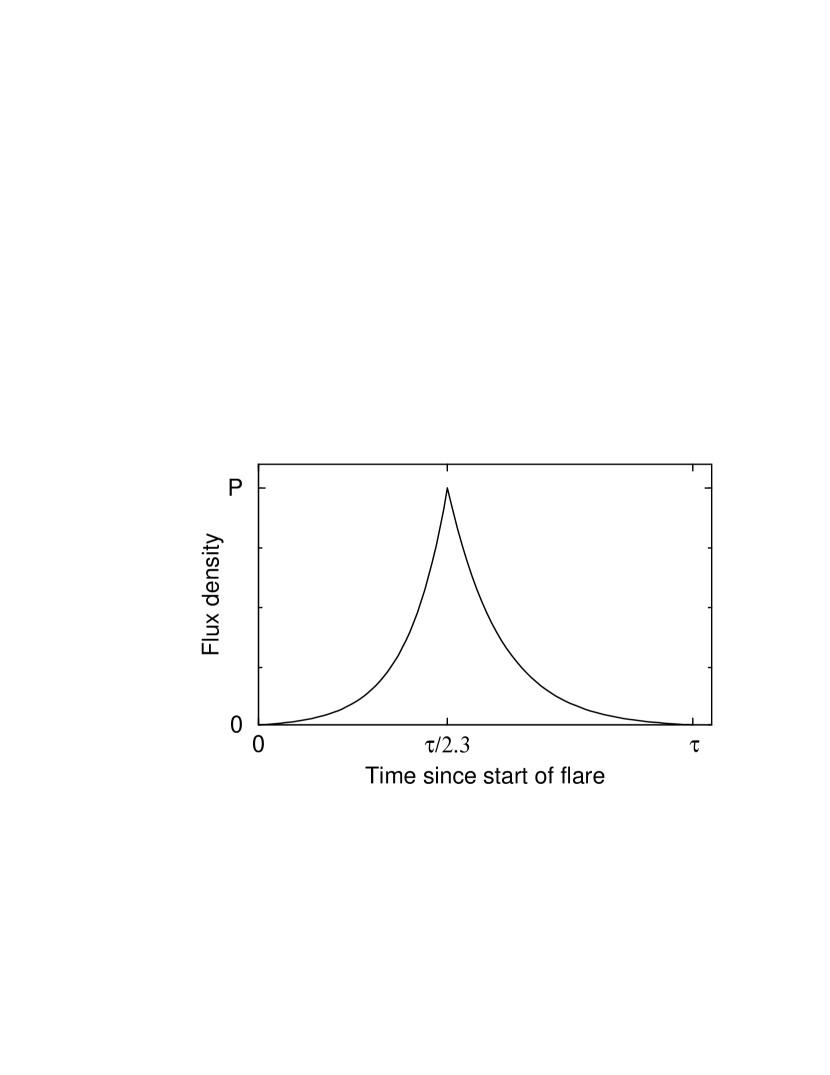
Figure 1: Canonical flare intensity profile used in simulated light curves, of the form $\bf\log{S}\propto t$, with $t_{\rm decay}=1.3\;t_{\rm rise}$. The flare intensity is plotted in units of the quiescent (non-flaring) flux density.

2.3 Flare timescales

It is difficult to obtain good observational constraints on the range of intrinsic timescales and amplitudes of AGN flares at radio wavelengths, since isolated flares are exceedingly rare, and the beaming factors are usually not well known. The majority of blazar light curves are composed of many different flares having a variety of timescales, so that often what appears to be a large isolated flare is actually a superposition of several smaller events.

Given these uncertainties, we let the flare lengths in our model be uniformly distributed over a range [$\tau_{min}$, $\tau_{max}$] in the rest frame of the jet. Since our estimate of the flare rate ($2\;\rm y^{-1}$) is based on bi-weekly monitoring data, and does not account for any flares with observed timescales $\mathrel{\hbox{\hbox to0.0pt{\hbox{\lower 4.0pt\hbox{$\sim$}}\hss}\hbox{$<$}}}1$ month we set $\tau_{min}=0.083$ y.

We derive a lower limit on $\tau_{max}$ by noting that there are no sources in either of the two major AGN monitoring campaigns (U. of Michigan or Metsähovi) that show a tendency to return to a quiescent baseline level in between flaring events. This implies that flares are of sufficient duration in the source frame so that AGNs are rarely observed in a non-flaring state. In our shot noise model, the probability of this occurring is approximately

$$p\simeq e^{-\rho\bar{\tau}/\delta},$$ (2)

where $\bar{\tau}\;=(\tau_{max}-\tau_{min})/2$ is the mean flare time scale in the source frame. We can estimate an upper limit on $\delta$ for the AGN parent population based on measurements of superluminal motion in samples of highly beamed AGNs (i.e., blazars). Jorstad et al. (2001a) find component velocities in the jets of gamma-ray loud blazars that range up to $\beta_{app}\simeq 30\;h^{-1}$. The relevant constraints from superluminal motion equations ($\beta_{app}<\Gamma$ and $\delta\mathrel{\hbox{\hbox to0.0pt{\hbox{\lower 4.0pt\hbox{$\sim$}}\hss}\hbox{$<$}}}2\Gamma$; see Urry & Padovani 1995) imply a maximum Doppler factor of $\sim 90$, assuming $h=0.65$. By choosing a reasonably low probability for being in a non-flaring state ($p=0.001$) and substituting $\delta=90$, $\rho=2\;\rm y^{-1}$ and $\tau_{min}=0.083\rm\;y$ in Eq. 2, we obtain $\tau_{max}\simeq 620$ y. Although this value is only a lower limit, we will show in § 4 that higher values of $\tau_{max}$ will simply increase the mean steady-state flux level of the overall parent population, and will not affect our main conclusions.

2.4 Flare Amplitudes

Given the observational uncertainties regarding the intrinsic flare amplitudes of AGNs, we will make the simple assumption that all flare amplitudes are the same fraction $P$ of a source’s rest frame quiescent flux level. Although this is likely a gross oversimplification in the case of real AGNs, our study is not concerned with low-amplitude flares, since they are not likely to affect the overall selection statistics of flux limited samples. Furthermore, we will show in § 3 that a broad intrinsic flare amplitude distribution is not needed to reproduce the basic properties of AGN light curves, since the effects of flare superposition and beaming can conspire to create a large range of observed flare amplitudes.

We constrain our flare amplitude parameter $P$ by examining the range of observed flux density in the long term ($\sim 20$ yr) light curves in the U. Michigan AGN sample. Of the 69 AGN light curves analyzed by Aller et al. (1999), the highest absolute peak-to-minimum flux ratio of any source at 4.8 GHz was $\sim 30$ for the BL Lac object 0235+164. Through repeated simulations of twenty-year light curves with various values of $P$, we find that for $P=0.05$, the probability of finding a peak-to-minimum ratio exceeding 30 in a highly beamed source ($\delta=90$) is $\mathrel{\hbox{\hbox to0.0pt{\hbox{\lower 4.0pt\hbox{$\sim$}}\hss}\hbox{$<$}}}0.001$. We therefore adopt $P=0.05$ in the simulations that follow.

3 Comparisons to AGN light curves

Having established the general parameters of our model, we are now able to compare our simulated light curves to those of actual AGNs. In Figure 2 we show the 20 year light curves of three AGNs at 4.8 GHz from the University of Michigan AGN monitoring program. In each panel the flux densities have been divided by the mean for comparison purposes. The top, middle and bottom panels show the light curves of the radio galaxy 3C 380, the quasar 3C 345, and the BL Lac object 0235+164, respectively.

Figure 2: Long-term light curves of three AGNs at 4.8 GHz, from monitoring observations at the University of Michigan Radio Observatory. The fluxes have been divided by the mean in each case.

Figure 3: Simulated radio light curves of three AGNs with redshifts and Doppler factors corresponding to the sources in Figure 2.

In order to make comparisons with our simulated light curves, estimates of the Doppler factors of these sources are needed. It is possible to use the measured apparent speed in the inner jet of 3C 380 ($\beta_{app}=10.6$ ; Polatidis & Wilkinson 1998) to obtain a crude estimate of its Doppler factor if we assume that the jet is viewed at an angle which maximizes its apparent velocity. This gives $\delta=\beta_{app}/\beta\simeq\beta_{app}\simeq 11$. The Doppler factor of 3C 345 has been well-constrained by Wardle et al. (1994), who modeled the three-dimensional motion of two components in its inner jet. They were able to constrain the viewing angle to $\theta\simeq 2\arcdeg$ and the Lorentz factor of the jet to be $\Gamma\mathrel{\hbox{\hbox to0.0pt{\hbox{\lower 4.0pt\hbox{$\sim$}}\hss}\hbox{$>$}}}20$, which implies $\delta\mathrel{\hbox{\hbox to0.0pt{\hbox{\lower 4.0pt\hbox{$\sim$}}\hss}\hbox{$>$}}}27$. The BL Lac object 0235+164 is the one of the most variable blazars in the U. Michigan monitoring sample, and is therefore likely to have a Doppler factor at the high end of the possible range ($\delta\sim 90$; see § 2.3). This source has also been constrained by Fujisawa et al. (1999) to have $\delta>80$ based on equipartition arguments and the ratio of observed inverse-Compton to synchrotron flux densities.

In Figure 3 we show three simulated light curves with Doppler factors and redshifts corresponding to the three AGNs in Figure 2. These light curves were calculated after allowing the sources to achieve a steady-state flaring level. The simulated flux densities have been divided by the mean in each case. We note that the source redshift will affect the timescales but not the amplitudes of our simulated light curves, since the flux densities are measured in units of the observed quiescent level. Our simulated curves reproduce the general variability characteristics of all three sources fairly well, even with our simplistic assumption of equal flare amplitudes.

A further comparison with the data can be made by examining the first order structure function of our simulated light curves. This function is defined as $D^{1}(\tau)=\left<[S(t)-S(t+\tau)]^{2}\right>$, where $S(t)$ is the flux density at time $t$ and $\tau$ is the time lag. Structure functions are commonly used as a means of characterizing the distribution of power in a stochastic process on different time scales (e.g., Simonetti, Cordes, & Heeschen 1985). The slope $b=d\log{D^{1}(\tau)}/d\log{\tau}$ is a general indicator of the type of stochastic process, with $b=0$ and $b=1$ corresponding to flicker and shot noise, respectively. As pointed out by Hughes et al. (1992), a slope of unity at long time lags is indicative of a shot-noise process of the type we are simulating. These authors found that the majority of the AGNs in the U. Michigan monitoring survey have structure function slopes that cluster near unity, with values ranging from approximately 0.7 to 1.65. In Figure 4 we show the structure function for the simulated light curve in the middle panel of Figure 3 with $\delta=27$ and $z=0.595$, corresponding to the properties of 3C 345. We find good agreement in the structure function slope of our model ($b=1.4$) and that measured by Hughes et al. (1992) at 4.8 GHz. The slope of our simulated structure function for 3C 345 is slightly steeper than the value of unity expected for a pure shot noise process, due to the Doppler contraction of flaring timescales in the observer’s frame, and the fact that we are modeling only major flares, which have a relatively low rate of occurence. The light curves of other AGNs may include longer-term, low amplitude flares that serve to flatten the slope of the structure function. We do not include these flares in our model, as they simply add a slowly varying component to the quiescent level, and do not have a major impact on the duty cycle of the source.

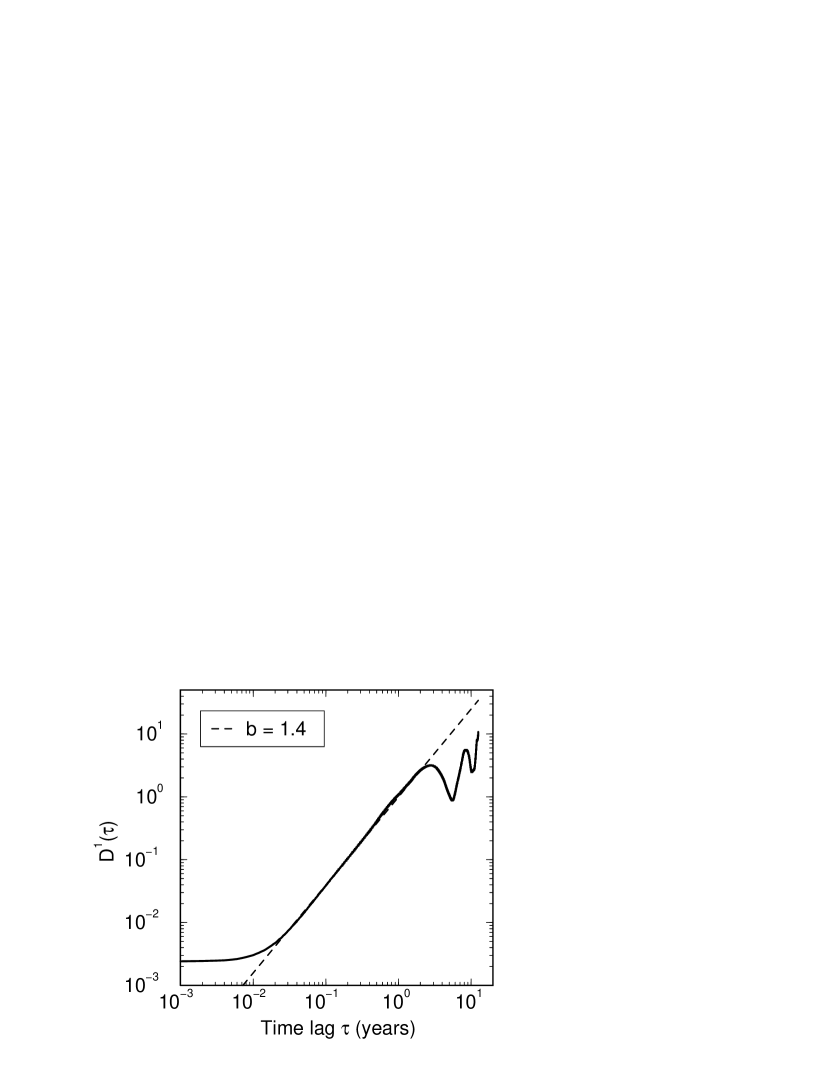
Figure 4: Structure function of the simulated light curve displayed in the middle panel of Figure 3, corresponding to the redshift and estimated Doppler factor of 3C 345. The fitted slope of 1.4 (dashed line) provides a good match to that of the observed structure function of 3C 345 at 4.8 GHz.

4 Variability duty cycles of beamed AGNs

An important quantity in the statistics of flaring source samples is the variability duty cycle, which we define to be the fraction of time the source spends above a particular flux density level. In this section we derive numerical estimates of AGN duty cycle functions by simulating light curves for sources with a wide range of Doppler factors and redshifts. A list of our individual model parameters is given in Table 1. For each set of parameters we simulate 500 twenty-year light curves, and generate a cumulative histogram that gives the fraction of time spent above a particular flux density $S$, measured in units of the observed quiescent flux density (in our case, $\delta^{2}S_{q}$). We plot the simulated duty cycles for sources at $z=1$ in Figure 5. It is apparent that relativistic beaming can have a large effect on the observed duty cycles of AGNs, especially for sources with $\delta\mathrel{\hbox{\hbox to0.0pt{\hbox{\lower 4.0pt\hbox{$\sim$}}\hss}\hbox{$>$}}}10$. As expected, these highly beamed jets tend to have a much wider range of observed variability amplitude than the more weakly beamed sources.

The cosmological redshifts of AGNs will stretch their intrinsic flux variations in time by a factor of $(1+z)$, and should therefore have an impact on their observed duty cycles as well. In Figure 6 we show the duty cycle functions of two simulated sources, one with $\delta=10$ (upper panel), and the other with $\delta=90$ (lower panel). The three curves in each panel represent the duty cycle of the source as it would appear at redshifts of 0, 1, and 3. For sources located at high redshifts, cosmological time dilation increases the probability that flares will overlap in the observer frame. This tends to increase the median flux density level of the source and shift the duty cycle curves to the right in Figure 6. A similar effect occurs when the maximum flare time scale is increased (Figure 7), since this will also increase the likelihood of overlapping flares. The net effect of raising $\tau_{max}$ is to boost the overall flux density levels of both strongly and weakly beamed sources alike. Although this will have implications on the intrinsic luminosity function of the parent population, it will not affect the statistics of flux-limited samples.

Our duty cycle simulations reveal a somewhat paradoxical property of AGN variability: although the flux densities of highly beamed sources can reach very high levels due to boosting, their flaring timescales are severely contracted, so that these sources are observed to spend most of their time in relatively low flaring states. Consequently, it is the weakly beamed sources that are more likely to be found in a state that is much higher than their quiescent level, due to the overlap of many long term flares. As we will show in the following section, this tends to slightly weaken the predicted effects of Doppler bias in flaring samples selected on the basis of relativistically beamed flux.

Figure 5: Observed variability duty cycle functions of an AGN at a redshift $z=1$ for different values of the jet Doppler factor ($\delta$). The curves from left to right represent values of $\delta=$ 90, 70, 50, 40, 30, 20, 10, 4, and 1, respectively. Each curve represents the fraction of time the source spends above a flux density $S$, measured in units of the observed quiescent (non-flaring) flux density ($\delta^{2}S_{q}$).

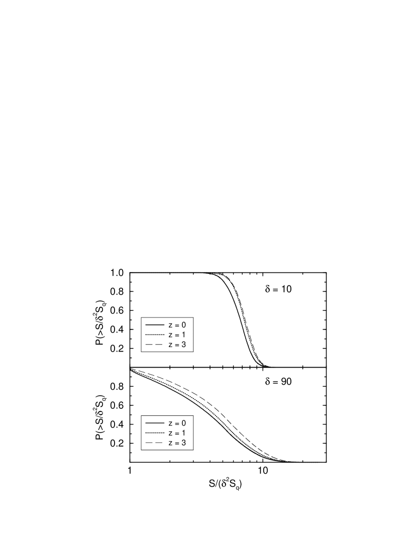
Figure 6: Plots showing the influence of source redshift on the duty cycle function of an AGN with Doppler factor 10 (top panel), and Doppler factor 90 (lower panel). The three curves in each panel represent the observed duty cycle function for the source at a redshift of $z=0$, 1 and 2, respectively. Sources at higher redshifts experience greater time dilation in the observer frame, which increases the probability of having flares that overlap in time. This tends to raise the median steady-state flux level of the source.

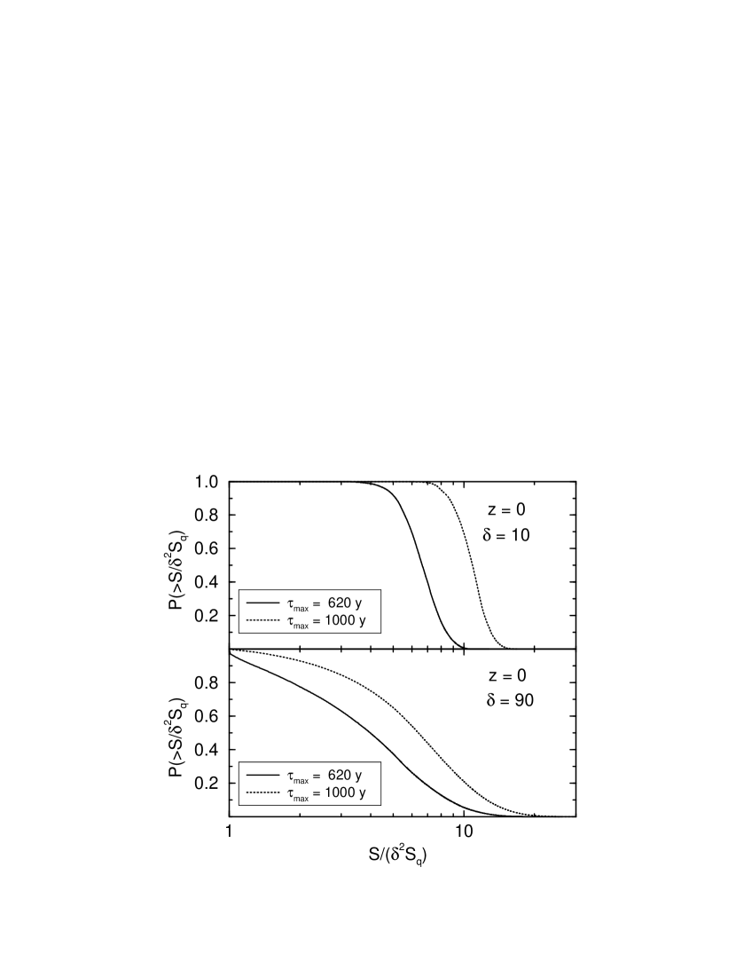
Figure 7: Plots showing the influence of maximum flare time scale on the duty cycle function of a source at redshift zero with Doppler factor 10 (top panel), and Doppler factor 90 (lower panel). Increasing the maximum time scale from 620 years to 1000 years raises the probability of having flares that overlap in time, which increases the median flux level of the source.

5 Effects of variability on core-selected AGN samples

The statistics of flux-limited samples should not be strongly influenced by flux variability as long as the variability properties of the parent population are relatively uniform. However, if some objects have a markedly different variability duty cycle than the rest of the population, this can affect the likelihood that they will appear in a flux-limited sample, thereby creating a selection bias.

In this section we investigate possible variability biases in flat-spectrum AGN samples by performing Monte Carlo simulations of both flaring and non-flaring beamed jet populations. We compare the observed properties of flux-limited samples drawn from these parent populations to determine to what degree core-selected AGN samples are additionally biased by source variability.

5.1 Simulated non-flaring jet population

In a previous study (Lister & Marscher 1997; Lister 1999), we successfully modeled the observed radio properties of a complete core-selected AGN sample (the Caltech-Jodrell Flat-spectrum survey; CJ-F) using a simulated population of two-sided, relativistically beamed jets. We found that the apparent jet velocity distribution of the CJ-F was best fit by a parent population of jets with a power-law Lorentz factor distribution that was weighted toward low speeds. This also appears to be the case for several other flat-spectrum AGN samples (e.g., Kellermann et al. 2000; Jorstad et al. 2001a) whose apparent velocity distributions are similar to that of the CJ-F.

For the purposes of this study we adopt the best-fit model of Lister (1999) for the CJ-F, which has no dependence of intrinsic luminosity on jet speed and $N(\Gamma)\propto\Gamma^{-1.25}$, with $1.001252\leq\Gamma\leq 45$. The jets have random spatial orientations and are distributed with a constant co-moving space density out to $z=4$. Their unbeamed 5 GHz luminosity function follows a fit to that of powerful (FR-II) radio galaxies, which incorporates pure exponential luminosity evolution (Urry & Padovani, 1995).

Since few constraints exist on the size of the CJ-F parent population, the lower cutoff of the parent luminosity function ($L_{1}$) is an important parameter. We can obtain an estimate of $L_{1}$ by examining the properties of the radio galaxy NGC 3894, which has the lowest 5 GHz luminosity of any source in the CJ-F sample. Its structure consists of a two-sided jet on parsec-scales, which has been monitored extensively by Taylor et al. (1998). By using the apparent expansion and flux density ratio of the jet and counter-jet, these authors found the viewing angle and jet speed to be $\theta\simeq 50\arcdeg$ and $\beta\simeq 0.3$, respectively. Assuming equal intrinsic luminosities and spectral index of zero for the jet ($j$) and counter-jet ($cj$), this implies that the radio luminosity of NGC 3894 is boosted by a factor of $(\delta_{j}^{p}+\delta_{cj}^{p})\simeq 2$, where we have assumed $p=2$, and $\delta_{j}=1.18$ and $\delta_{cj}=0.8$. Given that the observed 5 GHz luminosity of NGC 3894 is $1.9\times 10^{23}\;\rm W\;Hz^{-1}$ (Taylor et al., 1996), we will adopt a lower luminosity function cut-off of $9.5\times 10^{22}\;\rm W\;Hz^{-1}$ for our simulated non-flaring parent population.

In our Monte Carlo procedure we iteratively generate jets according to the above parameters until we obtain a sample of 293 sources with $S_{\rm 5\;GHz}>0.35$ Jy. These values correspond to the sample size and flux density cutoff of the CJ-F. Approximately $2\times 10^{6}$ parent objects are needed in a typical Monte Carlo run. In Lister & Marscher (1997) we required a substantially larger parent population ($\sim 10^{7}$ objects) to fit the CJ-F, since we used a smaller value of $L_{1}$ and a jet Lorentz factor distribution that only extended up to $15\;h^{-1}$.

We show the viewing angle and Doppler factor distributions for a single Monte Carlo run in Figure 8. As expected, the simulated CJ-F sample is heavily biased towards sources with low viewing angles since these tend to have the highest amount of Doppler boosting. The predicted Doppler factors of the CJ-F sources range up to the maximum possible value of $\sim 2\Gamma_{max}=90$.

Figure 8: Predicted distributions of jet viewing angle (left panel; log scale) and Doppler factor (right panel; linear scale) for the Caltech-Jodrell Flat-spectrum survey (CJ-F) based on a non-variable parent population.

5.2 Simulated flaring jet population

In order to simulate a flaring jet population, only slight modifications to our Monte Carlo model are necessary. We first assume that all of the parent objects have the same intrinsic variability characteristics given by the model parameters in Table 1. Although this is not likely true of the actual AGN population, this simplification makes it easier to isolate the effects of beaming on the statistics of flaring samples. Furthermore, the fact that radio variability is well-correlated with several other statistical beaming indicators (e.g., Aller et al. 1992; Lister et al. 2001) suggests that the observed variability characteristics of AGNs are more dependent on beaming than on intrinsic factors.

As in our previous Monte Carlo simulations, we simulate quiescent flux levels for the parent objects, but we now also assign a flaring level to each source based on its duty cycle function. We accomplish this by first binning the source into one of four redshift bins at $z$ = 0, 0.5, 1, 2, or 3, and then further binning it into one of thirteen sub-bins based on its Doppler factor. We then randomly generate a flare level according to the duty cycle (i.e., flaring probability) curve for the appropriate redshift/Doppler factor bin. The flux density of the source is then simply the quiescent flux density times the flaring level. If this flux density is fainter than the CJ-F cutoff, the source is discarded. We continue generating simulated sources in this manner until we obtain the necessary 293 sources with $S_{\rm 5\;GHz}>0.35$ Jy.

We note that it is necessary in these flaring simulations to modify the lower cutoff of the parent luminosity function, since we showed in § 4 that weakly beamed flaring sources are likely to be observed at levels considerably higher than their quiescent (non-flaring) level. Recalling that we used the least luminous source in the CJ-F (NGC 3894) to estimate $L_{1}$ in the non-flaring case, we estimate from our duty-cycle curves that its typical flaring level is approximately 7.4 times its quiescent level, given its redshift and Doppler factor. We therefore decrease $L_{1}$ by this factor and adopt a lower cutoff of $1.28\times 10^{22}\;\rm W\;Hz^{-1}$ for the quiescent luminosities of the simulated flaring population.

5.3 Comparison of flaring and non-flaring samples

In Figure 9 we show cumulative histograms of the predicted Doppler factor distribution for the CJ-F sample in the case of flaring (dashed line) and non-flaring (solid line) populations. The differences in the two cases are rather small, with the flaring sample being slightly more biased towards lower Doppler factors. There is also slightly less orientation bias present in the flaring sample (not shown), with relatively more sources found at higher viewing angles. We have verified these results using multiple Monte Carlo runs that all display the same effect. These findings are independent of our flaring amplitude parameter $P$, since increasing this parameter merely increases the overall flux density level of the entire parent population. This will not affect the selection statistics since increasing $P$ also requires that $L_{1}$ be adjusted downward accordingly.

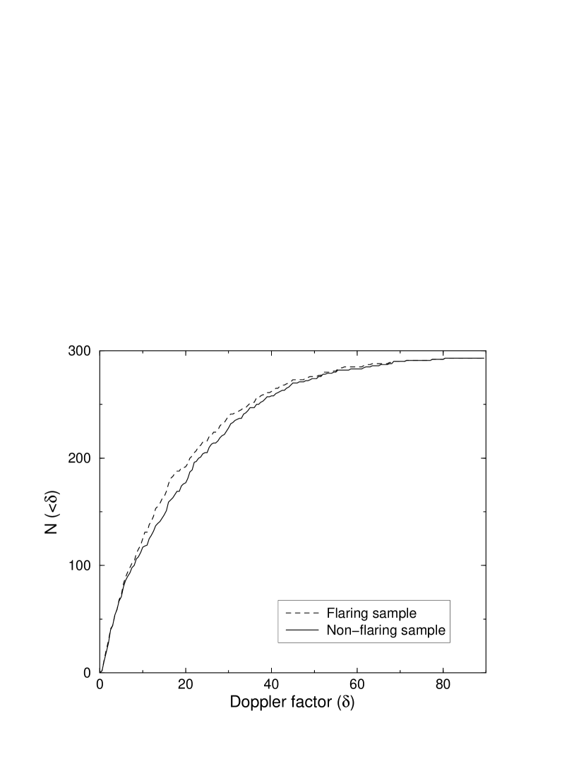
Figure 9: Predicted cumulative Doppler factor distributions for the CJ-F survey based on flaring (dashed line) and non-flaring (solid line) models. The sample selected from a flaring population is slightly more biased towards low-Doppler factor sources.

Although we have indeed found a bias in the statistics of flaring AGN samples, its predicted effects are rather small in medium-sized surveys such as the CJ-F. The main reason for this lies with the Lorentz factor distribution of the AGN population, which is weighted toward slow jets. The majority of the CJ-F parent objects are low-Doppler factor sources with jet axes inclined at $\sim 60\arcdeg$ from the line of sight. As we showed in § 4, the duty-cycle functions of these weakly-beamed objects are very similar, and are roughly symmetric about the mean steady-state level (Fig. 5). A sample composed predominantly of weakly-beamed flaring sources will therefore be statistically similar to a non-flaring sample, since the effects of variability will be averaged out.

Another important factor that reduces the size of the variability bias is the limited range of flux levels seen in individual AGNs at radio wavelengths (maximum peak/trough ratio $\sim 30$). By comparison, the entire parent population likely spans a flux density range of at least ten orders of magnitude, given the wide range of intrinsic luminosities, cosmological distances, and beaming factors that are present. Variability will therefore only influence the selection statistics of a relatively small fraction of the parent population that have fluxes near the survey limit. In large core-selected samples having a faint flux cutoff, these sources will tend to be weakly beamed, due to the predicted decrease in mean Doppler factor with flux density (see Lister 1999). As a result, the effects of variability will be statistically averaged out as described above. Those sources whose duty cycles are affected by beaming (with $\delta\mathrel{\hbox{\hbox to0.0pt{\hbox{\lower 4.0pt\hbox{$\sim$}}\hss}\hbox{$>$}}}10$) will tend to have beamed flux densities that are well above the survey limit, and will always be selected regardless of their flaring level. We have verified these effects by performing simulations using the same parent population as the CJ-F, only with a survey cutoff ten times fainter. We find virtually no statistical differences in the flaring and non-flaring samples, which contained approximately $\sim 3600$ sources.

6 Conclusions

We have developed a simple shot-noise variability model to examine how relativistic beaming affects the radio light curves and selection statistics of flat-spectrum AGNs. We summarize our main findings as follows:

1. Relativistic beaming will preferentially boost the amplitude of a flaring event with respect to an AGN’s quiescent flux level in the observer frame, and will also shorten its apparent time scale. As a result, highly beamed AGNs (i.e., with Doppler factors $\mathrel{\hbox{\hbox to0.0pt{\hbox{\lower 4.0pt\hbox{$\sim$}}\hss}\hbox{$>$}}}10$) are able to reach very high flux levels, but will in fact be observed to spend most of their time in relatively low flaring states.

2. The fact that the most highly beamed blazars are not observed to return to a quiescent level between flares suggests that the intrinsic timescales of individual flares are rather long, given the large Lorentz factors ($\Gamma\simeq 45$) of these jets that are inferred from superluminal motion studies. We find that the flare amplitudes must be a small fraction ($\mathrel{\hbox{\hbox to0.0pt{\hbox{\lower 4.0pt\hbox{$\sim$}}\hss}\hbox{$<$}}}5\%$) of the quiescent flux level in the source frame in order to reproduce the relatively small peak-to-trough flux density ratios seen in the most highly variable AGNs. The unbeamed counterparts of blazars should therefore have very stable radio light curves that are made up of a steady-state superposition of many long-term flares. The apparent “quiescent” flux density levels of these sources (identified in many unified models as radio galaxies) will be many times greater than their “true” quiescent (i.e., non-flaring) levels.

3. We have used the Monte Carlo beaming model of Lister & Marscher (1997) to model the parent population of the Caltech-Jodrell Flat-spectrum survey (CJ-F) using both flaring and non-flaring jets. We find that the standard orientation bias toward highly beamed jets with small viewing angles is predicted in both cases. In the case of a flaring population, however, the amount of orientation bias is slightly reduced due to the fact that the highly-beamed sources have a higher probability of being found in low flaring states. The magnitude of this effect is rather small in moderately-sized samples such as the CJ-F ($N\sim 300$ sources) due to the fact that the majority of the highly beamed sources in the parent population lie well above the survey flux limit and will be selected regardless of their flaring levels. We find that for larger samples with fainter cutoffs, any selection biases associated with variability should be negligible.

Table 1: AGN Variability Model Parameters

Symbol	Parameter	Value
$\rho$	Flaring rate	2 $\rm y^{-1}$
$\tau_{min}$	Minimum flare time scale	1 month
$\tau_{max}$	Maximum flare time scale	620 y
$P$	Peak-to-quiescent flux ratio of flare	1.05
$\delta$	Doppler factor	1, 2, 4, 6, 10, 20, 30, 40, 60, 70, 80, 90
$z$	Redshift	0, 0.5, 1, 2, 3

Note. — The flaring rate, time scale, and peak-to-quiescent ratio are all defined in the AGN rest frame.

References

- Aller et al. (1992) Aller, M. F., Aller, H. D. & Hughes, P. A. 1992, ApJ, 399, 16
- Aller et al. (1999) Aller, M. F., Aller, H. D., Hughes, P. A., & Latimer, G. E. 1999, ApJ, 512, 601
- Blandford & Königl (1979) Blandford, R. D. & Königl, A. 1979, ApJ, 232, 34
- Cruise & Dodds (1985) Cruise, A. M. & Dodds, P. M. 1985, MNRAS, 215, 417
- Fujisawa et al. (1999) Fujisawa, K., Kobayashi, H., Wajima, K., Hirabayashi, H., Kameno, S., & Inoue, M. 1999, PASJ, 51, 537
- Hartman et al. (1999) Hartman, R. C. et al. 1999, ApJS, 123, 79
- Hufnagel & Bregman (1992) Hufnagel, B. R. & Bregman, J. N. 1992, ApJ, 386, 473
- Hughes et al. (1992) Hughes, P. A., Aller, H. D., & Aller, M. F. 1992, ApJ, 396, 469
- Jorstad et al. (2001a) Jorstad, S. G., Marscher, A. P., Mattox, J. R., Wehrle, A. E., Bloom, S. D., Yurchenko, A. V. 2001a, ApJS, 134,181
- Jorstad et al. (2001b) Jorstad, S. G., Marscher, A. P., Mattox, J. R., Aller, M. F., Aller, H. D., Wehrle, A. E., and Bloom, S. D. 2001b, ApJ, in press
- Kellermann et al. (2000) Kellermann, K. I., Vermeulen, R. C., Zensus, J. A., Cohen, M. H. 2000, in Astrophysical Phenomena Revealed by Space VLBI, eds. H. Hirabayashi, P. G. Edwards, & D. W. Murphy (Sagamihara: Institute of Space & Astronautical Science), 159
- Lähteenmäki & Valtaoja (1999) Lähteenmäki, A. & Valtaoja, E. 1999, ApJ, 521, 493
- Lister (1999) Lister, M. L. 1999, Ph.D. thesis, Boston University.
- Lister & Marscher (1997) Lister, M. L. & Marscher, A. P. 1997, ApJ, 476, 572
- Lister et al. (2001) Lister, M. L., Tingay, S. J., & Preston, R. A. 2001, ApJ, 554, 964
- Perlmutter et al. (1999) Perlmutter, S. et al. 1999, ApJ, 517, 565
- Polatidis & Wilkinson (1998) Polatidis, A. G. & Wilkinson, P. N. 1998, MNRAS, 294, 327
- Scheuer & Readhead (1979) Scheuer, P. A. G. & Readhead, A. C. S. 1979, Nature, 277, 182
- Simonetti, Cordes, & Heeschen (1985) Simonetti, J. H., Cordes, J. M., & Heeschen, D. S. 1985, ApJ, 296, 46
- Taylor et al. (1996) Taylor, G. B., Vermeulen, R. C., Readhead, A. C. S., Pearson, T. J., Henstock, D. R., & Wilkinson, P. N. 1996, ApJS, 107, 37
- Taylor et al. (1998) Taylor, G. B., Wrobel, J. M., & Vermeulen, R. C. 1998, ApJ, 498, 619