Hard X–ray tails and cyclotron features in X–ray pulsars

Abstract

We review the physical processes occurring in the magnetosphere of accreting X–ray pulsars, with emphasis on those processes that give rise to observable effects in their high (E$>$10 keV) energy spectra. In the second part we compare the empirical spectral laws used to fit the observed spectra with theoretical models, at the light of the BeppoSAX results on the broad-band characterization of the X–ray pulsar continuum, and the discovery of new (multiple) cyclotron resonance features.

KEYWORDS: Magnetic fields — Stars: magnetic fields — Stars: neutron — pulsars: general — X–rays: stars

1. Introduction

An X–ray pulsar is, by definition, a celestial source showing pulsed emission when observed in X–rays. The very first pulsating X–ray source, Centaurus X–3, was discovered in 1971 by the first scientific X–ray satellite Uhuru [6]. Its 4.8 s pulse period implied a small emitting region, and because the object responsible for the pulsation is not destroyed by the centrifugal force it is necessary that at its surface the gravitational force is greater than the centrifugal one. This implies $\Omega_{p}\mathrel{\mathchoice{\vbox{\offinterlineskip\halign{\hfil$\displaystyle#$\hfil\cr<\cr\sim\cr}}}{\vbox{\offinterlineskip\halign{\hfil$\textstyle#$\hfil\cr<\cr\sim\cr}}}{\vbox{\offinterlineskip\halign{\hfil$\scriptstyle#$\hfil\cr<\cr\sim\cr}}}{\vbox{\offinterlineskip\halign{\hfil$\scriptscriptstyle#$\hfil\cr<\cr\sim\cr}}}}\sqrt{G\rho}$, where $\Omega_{p}$ is the pulse frequency, $G$ the gravitational constant, and $\rho$ the object mean density. The observed value of $\Omega_{p}$ implies $\rho\mathrel{\mathchoice{\vbox{\offinterlineskip\halign{\hfil$\displaystyle#$\hfil\cr>\cr\sim\cr}}}{\vbox{\offinterlineskip\halign{\hfil$\textstyle#$\hfil\cr>\cr\sim\cr}}}{\vbox{\offinterlineskip\halign{\hfil$\scriptstyle#$\hfil\cr>\cr\sim\cr}}}{\vbox{\offinterlineskip\halign{\hfil$\scriptscriptstyle#$\hfil\cr>\cr\sim\cr}}}}10^{7}$ g/cm³ and therefore the compact nature of the object responsible of the pulsed emission was established. The binary nature of Cen X–3 was soon after recognised by the observation of Doppler modulation in the observed pulse period [26]. The 2.1 day modulation was coincident with the periodic disappearing of the source X–ray flux, interpreted as eclipse of the compact object by the companion. Finally the optical counterpart was discovered as an early-type O star [10]. With all these elements it was possible to determine the mass of the compact object, which resulted to be 1.4 M_⊙: a neutron star (NS).

2. Physical processes in X–ray pulsars

The physical scenario able to explain the production of pulsed X–ray emission was elaborated by Shklovskii [27] before the discovery of Cen X–3. X–rays are produced in the conversion of the kinetic energy of the accreted matter (coming from the intense stellar wind of an early-type star — wind-fed binaries, or coming from an accretion disc due to Roche-lobe overflow — disk-fed binaries) into radiation, because of the interaction with the strong magnetic field of the NS, of the order of $10^{11}$–$10^{13}$ gauss. The dipolar magnetic field of the NS drives the accreted matter onto the magnetic polar caps, and if the magnetic field axis is not aligned with the spin axis, the NS acts as a “lighthouse”, giving rise to pulsed emission when the beam (or the beams, according to the geometry) crosses our line of sight.

For a detailed description of the spectral properties of accreting X–ray pulsars (AXPs) it is therefore necessary to describe the interactions of the X–rays produced at the NS surface with the highly magnetized plasma forming the magnetosphere. This is a formidable task because we cannot use a linearized theory for the radiative transfer equations but we have to deal with the fully magnetohydrodynamical system. This is due to the fact that the coupling constants among the interactions are so large that a series expansion is impossible.

This is the reason why there is not a parametrized description of AXP spectra in terms of physical quantities, but only empirical laws to fit the observed spectra. An alternative method is the numerical solution of the radiative transport equations assigning particular values to the physical parameters, comparing the obtained spectra with the observed ones, and varying the parameters until a match is reached.

2.1. Cyclotron resonant features

At some distance from the NS, that we will call magnetospheric radius $r_{m}$, the motion of the accreted matter will be dominated by its intense magnetic field. We define magnetosphere the region around the NS delimited by $r_{m}$. The electrons present in the magnetosphere will have an helicoidal motion along the magnetic field lines, with gyromagnetic (Larmor) frequency given by

$$\omega_{c}=\frac{eB}{\gamma mc}$$ (1)

where $\gamma$ is the Lorentz factor. For the magnetic field strength $B$ expected in the NS magnetosphere, the motion of the electron in the direction perpendicular to $B$ is quantized in the so-called Landau levels (see e.g. [13]). In the nonrelativistic case, the energy associated to each level is given by

$$\hbar\omega_{n}=n\,\hbar\omega_{c}$$ (2)

where $\omega_{c}$ is the Larmor gyrofrequency given in Eq. 1. As an aside, from Eq. 2 we have that $E_{n}=11.6\cdot B_{12}$ keV, where $B_{12}$ is the magnetic field strength in units of $10^{12}$ gauss. Therefore we expect to observe cyclotron features in the hard ($E>10$ keV) energy range. As we have seen, in the non-relativistic case the energy levels are harmonically spaced. When relativistic corrections are taken into account a slight anharmonicity is introduced in the Landau levels. Indeed, we have

$$\hbar\omega_{n}=mc^{2}\,\frac{\sqrt{mc^{2}+2n\hbar\omega_{c}\,\sin^{2}\theta}-1}{\sin^{2}\theta}$$ (3)

where $\theta$ is the angle between the line of sight and $B$.

Another consequence of the existence of the Landau levels is that an electromagnetic wave propagating in such a plasma will have well defined polarization normal modes, i.e. the medium will be birifringent [7]. It is not our intention to enter into the details of the propagation of waves in the magnetospheric plasma; we will develop a semi-quantitative approach by highlighting the plasma properties that have observable consequences in the AXP spectra.

If we introduce the complex refraction index $N$, with its real part the geometric refraction index and with its imaginary part the absorption coefficient, then the dispersion relation in the non-relativistic case can be written as a bi-quadratic equation in $N$. The solution for $N$ will have the form [13]

$$N_{1}^{2}\propto\frac{1}{\omega-\omega_{c}}\hskip 85.35826ptN_{2}^{2}\propto\frac{1}{\omega+\omega_{c}}\quad.$$ (4)

The wave with $N_{1}$ presents resonance and is right-handed circularly polarized (that is in the same sense as the electron gyration). This wave is called extraordinary, in opposition to the ordinary wave — described by $N_{2}$, which is left-handed circularly polarized. By introducing the complex refractive index is straightforward to obtain the cyclotron absorption cross section. By means of the optical theorem we obtain

$$\sigma_{c}=4\pi^{2}\alpha_{f}\frac{\hbar}{m}|e_{1}|^{2}\delta(\omega-\omega_{c})$$ (5)

where $\alpha_{f}=e^{2}/\hbar c$ is the fine structure constant, and $\vec{e_{1}}$ is the polarization versor of the extraordinary wave.

Up to now, we worked neglecting both relativistic corrections and thermal motions (cold plasma approximation). The release of the latter condition allows an electron to absorb waves not only of frequency $\omega=\omega_{c}$, but in the interval $\omega_{c}\pm\Delta\omega_{D}$, where the Doppler width is given by

$$\Delta\omega_{D}=\omega_{c}\sqrt{\frac{2kT}{mc^{2}}}\,|\cos\theta|$$ (6)

where $T$ is the electron temperature (we assumed a Maxwell-Boltzmann distribution for the electrons).

Once the electron absorbs a photon it (almost) immediately de-excitates on a time scale $t_{r}\sim 2.6\times 10^{-16}\,B_{12}^{-1}$ sec [13]. This has important consequences for the scattering cross sections. Indeed, while a scattering process involves two photons (one going in, one going out), absorption (or emission) processes involve only one photon. Therefore one expect that the two cross section are different. This is not true just because an absorbed photon is immediately re-emitted, and therefore the absorption-emission process is equivalent to a scattering. It is possible to show [13] that the cyclotron scattering cross section $\sigma_{\rm res}$ has the same form as the cyclotron absorption cross section $\sigma_{c}$ (Eq. 5) with the prescription

$$\delta(\omega-\omega_{c})\rightarrow\frac{\Gamma_{r}/2\pi}{(\omega-\omega_{c})^{2}+\Gamma_{r}^{2}/4}$$ (7)

where $\Gamma_{r}=\gamma_{r}\omega_{c}$, and $\gamma_{r}=(2/3)(e^{2}/mc^{3})\omega$ is the radiative damping.

Therefore photons with frequency close to $\omega_{c}$ will be scattered out of the line of sight, creating a drop in their number. Cyclotron “lines” observed in the spectra of AXPs are therefore not due to absorption processes, but are due to scattering of photons resonant with the magnetospheric electrons (as it occurs for the Fraunhofer lines in the Solar spectrum). This is why we will not use the term cyclotron lines but the more appropriate “cyclotron resonant features” (CRFs).

When relativistic effects are taken into account, it is possible to show that also ordinary waves show resonance, and are scattered out of the line of sight. Another important effect on the radiative properties of the plasma is due to a pure quantum effect: the so-called vacuum polarization. The magnetic field at which a quantum mechanical treatment of the plasma is necessary can be defined when the classical cyclotron energy $\hbar\omega_{c}$ becomes equal to the electron rest mass $mc^{2}$. That is

$$B_{cr}=\frac{m^{2}c^{3}}{e\hbar}=4.414\times 10^{13}\ {\rm gauss}\quad.$$ (8)

We call $B_{cr}$ the “critical” magnetic field strength. For $B$ not far from $B_{cr}$ virtual electron-positron pairs can be created. These virtual photons dominate the polarization properties of the plasma for frequencies in the range $\omega_{v1}\mathrel{\mathchoice{\vbox{\offinterlineskip\halign{\hfil$\displaystyle#$\hfil\cr<\cr\sim\cr}}}{\vbox{\offinterlineskip\halign{\hfil$\textstyle#$\hfil\cr<\cr\sim\cr}}}{\vbox{\offinterlineskip\halign{\hfil$\scriptstyle#$\hfil\cr<\cr\sim\cr}}}{\vbox{\offinterlineskip\halign{\hfil$\scriptscriptstyle#$\hfil\cr<\cr\sim\cr}}}}\omega\mathrel{\mathchoice{\vbox{\offinterlineskip\halign{\hfil$\displaystyle#$\hfil\cr<\cr\sim\cr}}}{\vbox{\offinterlineskip\halign{\hfil$\textstyle#$\hfil\cr<\cr\sim\cr}}}{\vbox{\offinterlineskip\halign{\hfil$\scriptstyle#$\hfil\cr<\cr\sim\cr}}}{\vbox{\offinterlineskip\halign{\hfil$\scriptscriptstyle#$\hfil\cr<\cr\sim\cr}}}}\omega_{v2}$, where [14, 15]

$$\omega_{v1}\simeq 3\,{\rm keV}\,\frac{\sqrt{n_{22}}}{B/0.1B_{cr}}\quad;\hskip 56.9055pt\omega_{v2}\simeq\omega_{c}$$ (9)

and therefore affect the scattering cross sections ($n_{22}$ is the electron density in units of $10^{22}$ cm^-3). In Fig. 1 we show the effects of the inclusion of vacuum polarization on the opacity (cross section times density) as obtained by [32].

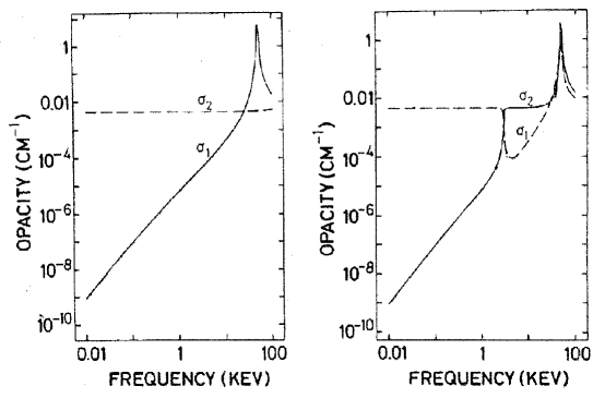
FIGURE 1.: Angle-averaged scattering opacities (cross section times density) for the extraordinary ($\sigma_{1}$) and ordinary ($\sigma_{2}$) modes, computed for $n_{22}=1$ and $\hbar\omega_{c}=50$ keV. Left: without vacuum polarization; Right: with vacuum polarization. From Ventura et al. (1979).

2.2. Continuum emission

The main physical process responsible for the continuum emission in AXPs is Compton scattering. We will not enter into the details of the problem of repeated scatterings in a finite, thermal medium (see e.g. [23]). Let us only summarize that an input photon of energy $E_{i}$ will emerge from a cloud of non-relativistic electrons (at a temperature $T$) with an average energy $E_{f}\sim E_{i}\,e^{y}$ (this is valid in the regime $E_{f}\ll 4kT$). The comptonization parameter $y$ therefore gives a measure of the photon energy variation in traversing the plasma, and is given by

$$y=\left\{\begin{array}[]{ll}\displaystyle\frac{4kT}{mc^{2}}\,\max\,(\tau,\tau^{2})&{\rm Nonrelativistic}\\ \\ \displaystyle\left(\frac{4kT}{mc^{2}}\right)^{2}\,\max\,(\tau,\tau^{2})&{\rm Relativistic}\\ \end{array}\right.$$ (10)

where $\max\,(\tau$, $\tau^{2})$ is nothing else but the average number of scattering suffered by the photons ($\tau$ is the optical depth of the medium). Note that if $E_{i}<4kT$ then photons can increase their energy at the expense of the electrons: this is inverse Compton scattering.

The detailed description of the spectrum of the emergent photons requires the solution of the Kompaneets equation, but it is possible to obtain qualitative information for special cases:

• $y\ll 1$ In this case only coherent scattering is important, and the emergent spectrum will be a blackbody spectrum or a “modified” blackbody spectrum according whether the photon frequency is lower or greater than the frequency at which scattering and absorption coefficients are equal [23].

• $y\gg 1$ Inverse Compton scattering can be important. If we define a frequency $\omega_{co}$ such that $y(\omega_{co})=1$, then for $\omega\gg\omega_{co}$ the inverse Compton scattering is saturated and the emergent spectrum will show a Wien hump, due to low-energy photons up-scattered up to $\hbar\omega\sim 3kT$ [23]. In the case in which there is not saturation a detailed analysis of the Kompaneets equation shows that the spectrum will have the form of a power law modified by a high energy cutoff [23, 29]. These two regimes are qualitatively depicted in Fig. 2.

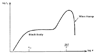
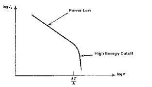
FIGURE 2.: Spectrum due Compton scattering in a thermal, nonrelativistic medium. Left: At low frequency the spectrum is blackbody, while at higher frequencies develops a Wien hump due to saturated inverse Compton. Right: Spectrum produced by unsaturated inverse Compton scattering (adapted from [23]).

3. Spectral X–ray observations of AXPs

3.1. Before BeppoSAX

The very first observation of a CRF in a spectrum of an X–ray pulsar was performed in 1978 when Trümper et al. [31] observed a $\sim$35 keV CRF in the spectrum of Hercules X–1. A while later it was observed not only the fundamental but also the first harmonics in the spectrum of the transient X–ray pulsar 4U0115+63 [33]. Observations of CRFs in other AXPs showed that they are a quite common phenomenon in this class of objects. But it was with the advent of the Japanese satellite Ginga that a systematic analysis of the spectra of AXPs was performed in search of CRFs. Mihara [16] analysed the spectra of 23 AXPs and found that 11 among them showed CRFs.

3.1.1. Continuum characterization

Because CRFs are broad features, the exact determination of the continuum is of paramount importance. From the analysis of the HEAO-1/A2 spectra of AXPs White et al. [34] found an empirical law that was able to fit their energy spectra

$${\rm POHI}(E)=\left\{\begin{array}[]{ll}E^{-\alpha}&E<E_{cut}\\ \displaystyle E^{-\alpha}\exp\left(-\frac{E-E_{cut}}{E_{f}}\right)&E>E_{cut}\end{array}\right.$$ (11)

It is evident that this model tries to simulate the unsaturated inverse Compton process shown in Fig. 2. But this model suffers the problem of a too abrupt break around the cutoff energy $E_{cut}$, problem enhanced by following more sensitive instruments. Therefore Tanaka [30] introduced a “smoother” cutoff of the form

$${\rm FDCO}(E)=\frac{1}{1+\exp{\displaystyle\left(\frac{E-E_{cut}}{E_{f}}\right)}}$$ (12)

that he called Fermi-Dirac cutoff because of it resemblance with the Fermi-Dirac distribution function. It is important to stress that the FDCO model does not have any physical meaning: it only gives a better description of the break in the AXP spectra.

Makishima and Mihara [11] were the first to note that in the AXPs showing CRFs there was a correlation between the cutoff energy $E_{cut}$ and the CRF energy $E_{c}$, namely $E_{c}\simeq(1.2-2.5)\cdot E_{cut}$. Therefore it seemed that the cutoff was in some way due to the presence of the CRF. The next step was performed by Mihara, who introduced the so-called NPEX (Negative Positive EXponential) model

$${\rm NPEX}(E)=(AE^{-\alpha}+BE^{+\beta})\exp\left(-\frac{E}{kT}\right)\quad.$$ (13)

This model is quite successful in describing the AXP spectra observed by Ginga in the 3–30 keV. Its components have also a physical meaning, because it mimics the saturated inverse Compton spectrum shown in Fig. 2 if $\beta=2$. Furthermore, because the (non relativistic) energy variation of a photon during Compton scattering is [23]

$$\frac{\Delta E}{E}=\frac{4kT-E}{mc^{2}}$$ (14)

then when $E=E_{c}$ the medium is optically thick and therefore $E_{c}\sim 4kT$.

3.1.2. CRF characterization

Mihara, besides the introduction of the NPEX model to describe the AXP continuum, introduced a new form for the CRF

$${\rm CYAB}(E)=\exp\left(-\frac{\tau(WE/E_{c})^{2}}{(E-E_{c})^{2}+W^{2}}\right)$$ (15)

which has the form of a Lorenzian of width $W$, and depth $\tau$. From a physical point of view, this is the form assumed by the cyclotron scattering cross section described by Eq. 7.

3.2. BeppoSAX observations of AXPs

With the advent of BeppoSAX the study of energy spectra of AXPs received new impulse because it was now possible to characterize with unprecedent detail the continuum on a broader energy range (0.1–200 keV), and the two high energy instruments aboard BeppoSAX, namely HPGSPC (sensitive in 5–60 keV; [12]) and PDS (15-200 keV; [5]), are the best suited for the detailed spectroscopy of CRFs. BeppoSAX observed all the persistent AXPs, plus a couple of transient ones (see Table 1). As a first result, we found that the NPEX model, successfully used to fit the Ginga data, is not adequate to describe the broad AXP continuum [3]. In particular we find that their continuum can be described in terms of (i) a black-body component with temperature of few hundreds eV; (ii) a power law of photon index $\sim$1 up to $\sim$10 keV; and a (iii) a high energy ($\mathrel{\mathchoice{\vbox{\offinterlineskip\halign{\hfil$\displaystyle#$\hfil\cr>\cr\sim\cr}}}{\vbox{\offinterlineskip\halign{\hfil$\textstyle#$\hfil\cr>\cr\sim\cr}}}{\vbox{\offinterlineskip\halign{\hfil$\scriptstyle#$\hfil\cr>\cr\sim\cr}}}{\vbox{\offinterlineskip\halign{\hfil$\scriptscriptstyle#$\hfil\cr>\cr\sim\cr}}}}$10 keV) cutoff that makes the spectrum rapidly drop above $\sim$40–50 keV.

Source	Obs Date	Ecyc (keV)	FWHM (keV)	References
4U0115+63 (M)	20 Mar 1999	$12.78\pm 0.08$	$3.58\pm 0.33$	[25]
4U1538–52 (M)	29 Jul 1998	$21.5\pm 0.4$	$6.7\pm 1.2$	[22]
Cen X–3 (M?)	27 Feb 1997	$28.5\pm 0.5$	$7.3\pm 1.9$	[24]
XTE J1946+27	09 Oct 1998	$33\pm 4$	$16\pm 2$	[26]
OAO1657–415	04 Sep 1998	$36\pm 2$	10	[17]
4U1626–67	06 Aug 1996	$38.0\pm 0.9$	$11.8\pm 1.7$	[19]
4U1907+09 (M)	29 Sep 1997	$38.3\pm 0.7$	$9.7\pm 2.3$	[1]
Her X–1	27 Jul 1996	$42.1\pm 0.3$	$14.7\pm 1.1$	[2]
GX301–2 (M)	24 Jan 1998	$49.5\pm 1.0$	$17.9\pm 2.5$	[20]
Vela X–1 (M)	14 Jul 1996	$54.8\pm 0.9$	$25.0\pm 2.1$	[18]
GX1+4	25 Mar 1997	…	…	[9]
GS1843+00	04 Apr 1997	…	…	[21]
X Persei	09 Sep 1996	…	…	[4]
M stands for multiple lines detected/suspected

TABLE 1.: BeppoSAX observations of X–ray binary pulsars

Furthermore, the CRFs observed with BeppoSAX are better described in terms a Gaussian in absorption, defined as [28]

$${\rm GAUABS}(E)=\left[1-I\exp\left(-\frac{(E-E_{c})^{2}}{2W^{2}}\right)\right]\quad.$$ (16)

In order to better characterize the CRF we introduced a new tool, the so-called normalized Crab ratio. The Crab ratio is simply the ratio between the source count rate spectrum and the count rate spectrum of the Crab Nebula. As this second spectrum is known, with great accuracy, to be free of features and to be modeled at first order with a power law in a very broad energy range, this ratio is quite well suited to enhance the presence of features in the spectrum. Furthermore the ratio is in first approximation independent from the calibration of the instrument.

In order to enhance the deviations from the continuum we multiply the ratio by a E^-2.1 power law, that is the functional form of the Crab Nebula spectrum, and we divide by the functional describing the continuum shape of the source (from this the name normalized Crab ratio). The procedure is described in Fig. 3 where we plot the result of each different step used to obtain the final result in the case of 4U0115+63. Note the presence of up to four cyclotron harmonics in the spectrum [25].

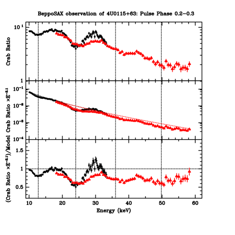
FIGURE 3.: Normalized Crab ratio for the BeppoSAX observation of the transient AXP 4U0115+63. Both the two high energy instruments, HPGSPC (black marks) and PDS (grey marks), are shown. Note the presence of at least four cyclotron harmonics [25].

By performing the normalized Crab ratio on all the AXPs listed in Table 1 it is immediate to observe that higher the CRF energy, broader the feature [3]. The correlation between $E_{c}$ and the CRF FWHM is quite evident in Fig. 4, and is easily understood in terms of Doppler broadening of the electrons responsible of the resonance, and holds for all the sources displaying single CRFs (see Eq. 6). It is important to stress that this relation does not hold in presence of multiple harmonics. In other words, it seems that the temperature of the electrons responsible of higher CRF harmonics is different from that of the electrons responsible of the fundamental CRF. From Fig. 4 and by means of Eq. 6 we derived that the electron temperature responsible for the resonance is in the range $\sim$15–30 keV. This energy range is somehow “critical”, because in some AXPs (and the effect is particularly evident in OAO1657–40 [17]) we observe actually two changes of slope in the high energy part of their spectra: a first change of slope occurs in the $\sim$10–20 keV range, while a second steepening occurs for higher energies. This leds to our last issue: “anomalous” multiple CRFs.

FIGURE 4.: FWHM vs centroid energy for the cyclotron features observed by BeppoSAX and listed in Table 1. We include the OSSE measurement on the 1994 outburst of A0535+26 [8]. Note that the linear correlation has been computed without taking into account the A0535+26 point.

There are three sources, namely 4U1907+09, Vela X–1, and GX301–2 that require two CRFs in their energy spectra. The anomaly is that (i) the two CRFs are not harmonically spaced; (ii) the depth of the “fundamental” is much smaller than that of its “harmonics”, (iii) their width does not correlate with their centroid energy and, more importantly, (iv) there is no trace of the “fundamental” in the normalized Crab ratio. Because of this last point we have some doubt about the interpretation of them as CRF, expecially because they are all in the critical energy range 10–30 keV where we observe the change of slope in the continuum. We are therefore inclined to interpret them as due to a not correct modelization of the continuum. Another possible explanation could be that they are due to vacuum polarization effects (see Fig. 1), but this interpretation requires a more quantitative analysis. For the three sources discussed above, we did not plot in Fig. 4 the “anomalous” CRF but the one obtained from the normalized Crab ratio.

4. Conclusions

The broad-band capabilities of BeppoSAX have shown that the simple phenomenological spectral laws used to describe AXP spectra in narrow energy ranges are inadequate to fit broad-band spectra. The study of AXPs as a class has shown that there is a critical region between $\sim$10 and $\sim$30 keV in which we observe a change of slope in the continuum. If not well modeled this could give rise to extraneous features that could be interpreted as CRF. Probably a detailed treatment of Compton scattering taking into account the effects of the magnetic field could help to solve this issue. Also vacuum polarization effects could alter the emergent energy spectra and explain the observed “anomalous” CRF harmonics.

Doppler broadening of the electrons responsible for the CRF is able to explain the observed correlation between CRF FWHM and centroid energy, showing that the electron temperature is in the range 15–30 keV for all the observed AXPs. This correlation does not hold for sources showing multiple CRFs, implying that the temperature of the electrons giving rise to higher harmonics could be different.

Acknowledgements We wish to thank the “X–ray pulsar fans” working group, formed by the friends at the TeSRE, IFCAI and ESTEC/SSD institutes in Bologna, Palermo and Noordwijk, who produced a good wealth of results on BeppoSAX observations and without whom this work would not have been possible.

References

- [1] Cusumano, G., et al. 1998, A&A, 338, L79
- [2] Dal Fiume, D., et al. 1998, A&A, 329, L41
- [3] Dal Fiume, D., et al. 2000, ASR, 25, 399
- [4] Di Salvo, T., et al. 1998, ApJ, 509, 897
- [5] Frontera, F., et al. 1997, A&AS, 122, 357
- [6] Giacconi, R., et al. 1971, ApJ, 167, L67
- [7] Ginzburg, V.L. 1970, The Propagation of Electromagnetic Waves in Plasmas, Pergamon Press, Oxford
- [8] Grove, J.E., et al. 1995, ApJ, 438, L25
- [9] Israel, G.L., et al. 1998, Nucl. Phys. B (Proc. Suppl.), 69, 141,
- [10] Krzeminski, W. 1974, ApJ, 192, L135
- [11] Makishima, K., & Mihara, T. 1992, in Frontiers of X–ray Astronomy, eds. Tanaka, Y., & Koyama, K. Universal Academy Press, Tokyo, p. 23
- [12] Manzo, G., et al. 1997, A&AS, 122, 341
- [13] Mészáros, P. 1992, High-Energy Radiation from Magnetized Neutron Stars, Chicago University Press
- [14] Mészáros, P., & Ventura, J. 1978, Phys.Rev.Lett., 41, 1544
- [15] Mészáros, P., & Ventura, J. 1979, Phys.Rev., D19, 3565
- [16] Mihara, T. 1995, PhD thesis, RIKEN
- [17] Orlandini, M., et al. 1999, A&A, 349, L9
- [18] Orlandini, M., et al. 1998, A&A, 332, 121
- [19] Orlandini, M., et al. 1998, ApJ, 500, L163
- [20] Orlandini, M., et al. 2000, ASR, 25, 417
- [21] Piraino, S., et al. 2000, A&A, 357, 501
- [22] Robba, N.R. et al. 1999, in preparation
- [23] Rybicki, G.B., & Lightman, A.P. 1975, Radiative Processes in Astrophysics, John Wiley & Sons
- [24] Santangelo, A., et al. 1998, A&A, 340, L55
- [25] Santangelo, A., et al. 1999, ApJ, 523, L85
- [26] Schreirer, E., et al. 1972, ApJ, 172, L79
- [26] Segreto, A. et al. 1999, in preparation
- [27] Shklovskii, I.S. 1967, ApJ, 148, L1
- [28] Soong, Y., et al. 1990, ApJ, 348, 641
- [29] Sunyaev, R.A., & Titarchuk, L.G. 1980, A&A, 86, 121
- [30] Tanaka, Y. 1986, in Radiation Hydrodynamics in Stars and Compact Objects, eds. Mihalas, D., & Winkler, K.H. Springer, Berlin, p. 198
- [31] Trümper, J., et al. 1978, ApJ, 219, L105
- [32] Ventura, J., et al. 1979, ApJ, 233, L125
- [33] Wheaton, W.A., et al. 1979, Nat, 282, 240
- [34] White, N.E., et al. 1983, ApJ, 270, 711