The dependence of cosmological parameters estimated from the microwave background on non-gaussianity

Abstract

The estimation of cosmological parameters from cosmic microwave experiments has almost always been performed assuming gaussian data. In this paper the sensitivity of the parameter estimation to different assumptions on the probability distribution of the fluctuations is tested. Specifically, adopting the Edgeworth expansion, I show how the cosmological parameters depend on the skewness of the $C_{\ell}$ spectrum. In the particular case of skewness independent of $\ell$ I find that the primordial slope, the baryon density and the cosmological constant increase with the skewness.

I Introduction

The new generation of cosmic microwave background (CMB) experiments (see e.g. lee ; halverson ; net , and the future missions Planck planck , and Map map ) promises to estimate the cosmological parameters within a precision of 1%. The current dataset already allows in some cases an uncertainty below 10% on such parameters as the baryon density or the primordial spectral slope. Such a precision allows and demands a clear assessment of the theoretical assumptions.

So far, all the estimations of cosmological parameters based on the CMB data assumed a Gaussian distribution of the primordial fluctuations (the only exception I know of is Ref. cont in which the primordial slope $n$ was estimated in presence of skewness). Such an assumption is based on the conventional models of inflation and has the obvious and enormous advantage of being simple and uniquely determined. However, the gaussianity of the primordial temperature fluctuations is still to be fully tested ban ; kogut ; mag and there exist several theoretical models which actually predict its violation falk . Therefore, it is necessary to quantify how the cosmological parameters derived from CMB experiments depend on the statistical properties of the fluctuation field.

In this paper I derive the dependence of four cosmological parameters on the skewness of the fluctuations assuming a flat space. The parameters are the primordial slope $n$, the baryon and cold dark matter rescaled density parameters $\omega_{b}\equiv\Omega_{b}h^{2},\omega_{c}\equiv\Omega_{c}h^{2}$ ( $h$ is the Hubble constant in units of 100 km/sec/Mpc), and the cosmological constant density parameter $\Omega_{\Lambda}$. The flat space constraint reduces to the relation $h^{2}=(\omega_{b}+\omega_{c})/(1-\Omega_{\Lambda}).$

It is clear that removing the hypothesis of Gaussianity leaves room for an infinity of different possible assumptions concerning the fluctuation distribution. I adopt here the Edgeworth expansion (EE), for three reasons: a) it can be seen as a perturbation of a Gaussian function; b) it is easy to manipulate analytically and c) it is the distribution followed by any random variable that is a linear combination of $N$ random variables in the limit of large $N$ (for $N\rightarrow\infty$ the Edgeworth distribution reduces to a Gaussian). The latter property might be useful to describe fluctuations that arise due to several independent sources. The EE has been previously used in cosmology to model small deviations from Gaussianity ame94 ; ame96 ; ju ; fos ; ameastro .

The main drawback of the EE is that it is not positive definite. However, when the deviation from Gaussianity is small, this problem is pushed many standard deviations away from the peak and does not affect the parameter estimation.

This paper is meant to exemplify the effects that a non-zero skewness introduces on the likelihood estimation. For generality, I will not confine myself to any specific mechanism for generating the non-gaussianity. Moreover, for simplicity, I will skip over several additional complications like bin cross-correlations, calibration, pointing and beam errors that an accurate analysis should take into account.

II Edgeworth likelihood

The likelihood function usually adopted in CMB studies (e.g. bon ; lee ; halverson ; net ) is an offset log-normal function. This function is an approximation to the exact likelihood that holds for Gaussian data in presence of Gaussian noise bon . The offset depends on quantities that are not yet publicly available; since the offset can be neglected in the limit of small noise, we assume as starting point a simple log-normal that, neglecting factors independent of the variables, can be written as

$$-2\log L(\alpha_{j})=\sum_{i}\frac{Z_{\ell,t}(\ell_{i};\alpha_{j})-Z_{\ell,d}(\ell_{i})}{\sigma_{\ell}^{2}},$$ (1)

where $Z_{\ell}\equiv\log\hat{C}_{\ell}$, the subscripts $t$ and $d$ refer to the theoretical quantity and to the real data, $\hat{C}_{\ell}$ are the spectra binned over some interval of multipoles centered on $\ell_{i}$, $\sigma_{\ell}$ are the experimental errors on $Z_{\ell,d}$, and the parameters are denoted collectively as $\alpha_{j}$. We neglect also the residual correlation between multipole bins, which should be anyway very small for the latest data. An overall amplitude parameter $A$ can be integrated out analytically adopting a logarithmic measure $d\log A$ in the likelihood. Writing $\hat{C}_{\ell}=A\hat{C}_{\ell}^{\prime}$ it follows $Z_{\ell,t}=\log A+\log\hat{C}_{\ell,t}^{\prime}=\log A+Z_{\ell,t}^{\prime}$ so that, neglecting the factors independent of the variables and putting $w=\log A$, we obtain

$$L\propto\int\exp\left[-\sum_{\ell}\frac{\left[w+\Delta_{\ell}\right]^{2}}{2\sigma_{\ell}^{2}}\right]dw\propto e^{-\frac{1}{2}\left(\gamma-\frac{\beta^{2}}{\alpha}\right)},$$ (2)

where

$$\Delta_{\ell} = Z^{\prime}_{\ell,t}(\ell_{i};\alpha_{j})-Z^{\prime}_{\ell,d}(\ell_{i}),$$

$$\alpha = \sum 1/\sigma_{\ell}^{2},\quad\beta=\sum\Delta_{\ell}/\sigma_{\ell}^{2}.$$

$$\gamma = \sum\Delta_{\ell}^{2}/\sigma_{\ell}^{2}.$$

Let us now introduce the Edgeworth expansion. Denoting with $x_{\ell}=\left(w+\Delta_{\ell}\right)/\sigma_{\ell}$ the normal variable in the Gaussian function, the Edgeworth expansion is kendall

$$P(x_{\ell})=\exp\left[-\frac{x^{2}_{\ell}}{2}\right]\left[\right.1+\frac{k_{3,\ell}}{6}H_{3}(x_{\ell})+$$

$$\frac{k_{4,\ell}}{24}H_{4}(x_{\ell})+\frac{k_{3,\ell}^{2}}{72}H_{6}(x_{\ell}) +...,\left.\right],$$ (3)

where $k_{n,\ell}$ is the $n$-th cumulant of $x_{\ell}$ and $H_{n}$ is the Hermite polynomial of $n$-th order. Notice that the EE has the same norm, mean and variance as the Gaussian, but different mode (the peak of the distribution). Here, as a first step, we limit ourselves to the first non-Gaussian term containing the skewness $k_{3,\ell}$.

Assuming that $x_{\ell}$ is distributed according to the Edgeworth expansion, we can build the truncated Edgeworth likelihood function ameastro to first order in $k_{3,\ell}$:

$$L=e^{-\sum_{\ell}\frac{x^{2}_{\ell}}{2}}\left[1+\frac{\kappa_{3,\ell}}{6}\sum_{\ell}H_{3}(x_{\ell})\right],$$

with $H_{3}(x_{\ell})=x_{\ell}^{3}-3x_{\ell}$. Now, integrating over $w$ we obtain

$$L=\int e^{-\sum\frac{x^{2}_{\ell}}{2}}\left[1+\frac{1}{6}\sum k_{3,\ell}H_{3}(x_{\ell})\right]dw=$$

$$\sqrt{\frac{2\pi}{\alpha}}e^{-\frac{1}{2}\left(\gamma-\frac{\beta^{2}}{\alpha}\right)}\left[1+\frac{1}{6}g(k_{3,\ell},\Delta_{\ell},\sigma_{\ell})\right],$$ (4)

where

$$\alpha^{3}g(k_{3,\ell},\Delta_{\ell},\sigma_{\ell})=(-3\alpha\beta-\beta^{3})\sum\frac{k_{3,\ell}}{\sigma_{\ell}^{3}}$$

$$+(3\alpha^{2}+3\alpha\beta^{2})\sum\frac{k_{3,\ell}\Delta_{\ell}}{\sigma_{\ell}^{3}}-3\alpha^{2}\beta\sum k_{3,\ell}\left(\frac{\Delta^{2}_{\ell}}{\sigma_{\ell}^{3}}-\frac{1}{\sigma_{\ell}}\right)$$

$$+\alpha^{3}\sum k_{3,\ell}\left(\frac{\Delta^{3}_{\ell}}{\sigma_{\ell}^{3}}-3\frac{\Delta_{\ell}}{\sigma_{\ell}}\right).$$

This is the likelihood function that we study below. The effect of the extra terms is to shift the peak (or mode) of the distribution of each $C_{\ell}$ while leaving the mean unperturbed. Since the shift depends on $\Delta_{\ell}$ ,$\sigma_{\ell}$ and $k_{3,\ell}$, the resulting mode spectrum will be distorted with respect to the mean spectrum. Therefore, the likelihood maximization will produce in general results that depend on $k_{3,\ell}$. In Fig. 1 we show the peak shift introduced in the simplified case in which the skewness is independent of $\ell$: if $k_{3}$ is negative, the spectrum is shifted upward by a larger amount at the very small and very large multipoles, and by a smaller amount around $\ell=200$, where the relative errors are the smallest; if $k_{3}$ is positive the shift is downward. As a consequence of the distortion, we expect that a constant negative skewness favours spectra which are tilted downward with respect to the Gaussian case, and the contrary for a positive skewness. In general, the cosmological parameters will depend on the multipole dependence of $k_{3,\ell}$. For small $k_{3}\sigma_{\ell}$, the shift can be approximated by

$$C_{\ell\,(mode)}=C_{\ell(mean)}(1-k_{3}\sigma_{\ell}/2).$$ (5)

Clearly, if the peak shift introduced by the EE were independent of $\ell$, the integration over the amplitude $w$ would erase the non-gaussian effect on the likelihood. That is, putting $\sigma_{\ell}$ and $\Delta_{\ell}$ equal to a constant independent of $\ell$ we obtain $g(k_{3,\ell},\Delta_{\ell},\sigma_{\ell})=0.$

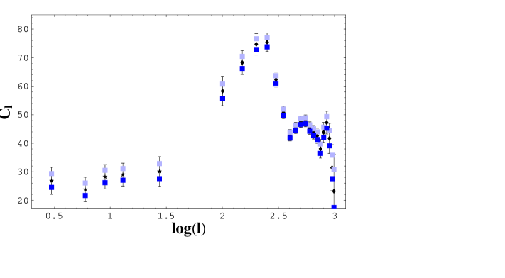
Figure 1: The squares mark the mode of the $C_{\ell}$ distribution for $k_{3}=-2$ (light squares), and for $k_{3}=2$ (dark squares). The data are from Cobe and Boomerang.

III Dependence on the skewness

To evaluate the likelihood, a library of CMB spectra is generated using CMBFAST sel . Following net I adopt the following uniform priors: $n\in(0.7,1.3),$ $\quad\omega_{b}\in(0.0025,0.08),\quad$ $\omega_{c}\in(0.05,0.4),\Omega_{\Lambda}\in(0,0.9)$. As extra priors, the value of $h$ is confined in the range $(0.45,0.9)$ and the universe age is limited to $>10$ Gyr. The remaining input parameters requested by the CMBFAST code are set as follows: $T_{cmb}=2.726K,$ $Y_{He}=0.24,N_{\nu}=3.04,\tau_{c}=0.$ In the analysis of net $\tau_{c}$, the optical depth to Thomson scattering, was also included in the general likelihood and, in the flat case, was found to be compatible with zero at slightly more than 1$\sigma$ . Therefore here, to reduce the parameter space, I assume $\tau_{c}$ to vanish. The theoretical spectra are compared to the data from COBE bon and Boomerang net .

To specify the skewness $k_{3,\ell}$ three simplified cases are studied: in the first one (“constant skewness”), $k_{3,\ell}=k_{3}^{*}$ is assumed independent of the multipole $\ell$; in the second (“gaussian skewness”), the skewness is assumed to be generated by some process only in a particular range of multipoles:

$$k_{3,\ell}=k_{3}^{*}e^{-(\ell-\ell^{*})^{2}/2\Delta^{*2}_{\ell}},$$ (6)

where, in the numerical examples below, I put $\ell^{*}=200$ and $\Delta_{\ell}^{*}=20$. In the third case (“hierarchical skewness”), the “hierarchical” ansatz is assumed peeb , in which the skewness of the temperature field is proportional to the square of its variance. At the first order, we can assume that the skewness of the $C_{\ell}$ distribution is proportional to the skewness of the fluctuation field, so I put

$$k_{3,\ell}=k_{3}^{*}\left(C_{\ell}/C^{*}\right)^{2},$$ (7)

where, for instance, $C^{*}=C_{200}$. In all three cases $k^{*}_{3}$ is left as a free parameter. These three choices are of course purely an illustration of what a real physical mechanism might possibly produce.

Fig. 2 shows the one-dimensional Edgeworth likelihood functions marginalized in turn over the other three parameters. For the “constant skewness”, $k_{3}^{*}$ varies from -1.6 to 1.2 ( light to dark curves): below and above these values the likelihood begins to show pronounced negative wings, which signals that the first order Edgeworth expansion is no longer acceptable. While the likelihood for $\omega_{c}$ is almost independent of $k_{3}$ , it turns out that the other likelihoods move toward higher values for higher skewness. As anticipated, this can be explained by observing that a higher skewness implies smaller $C_{\ell}$ at small multipoles: a tilt toward higher $n$ and higher $\omega_{b}$ gives therefore a better fit. The effect is of the order of 10% for $k_{3}^{*}\approx 1$.

In the “gaussian skewness” case the trend is qualitatively the opposite, as can be seen in Fig. 3, where $k_{3}^{*}$ ranges from -4 to 4 (light to dark). Here the cosmological parameters decrease for an increasing skewness. The reason is that now the effect is concentrated around the intermediate multipoles $\ell\approx 200$: a positive skewness induces smaller $C_{\ell}$ at these multipoles, and therefore a smaller $n$ and $\omega_{b}$ helps the fit. The third case, the “hierarchical skewness”, is not shown because is qualitatively similar to the previous case: the region around $\ell=200$ is in fact also the region where $C_{\ell}$ is larger and therefore $k_{3,\ell}$ given by Eq. (7) is larger.

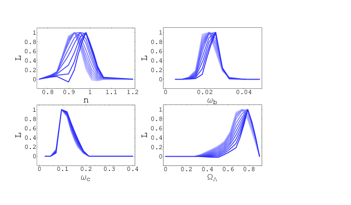
Figure 2: Likelihood functions for the four cosmological parameters in the constant skewness case. The skewness increases from -1.6 to 1.2, light to dark.

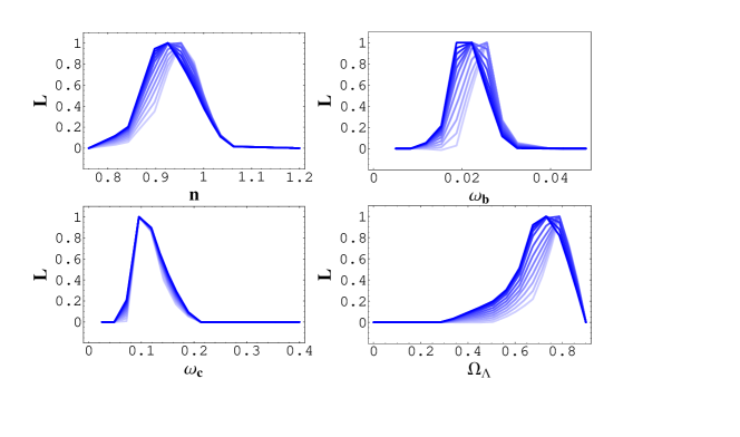
Figure 3: Likelihood functions for the four cosmological parameters in the “gaussian skewness” case. The skewness increases from -4 to 4, light to dark.

Fig. 4 summarizes the results: the trend of the estimated parameters (mean and standard deviation) versus $k^{*}_{3}$ in the “constant skewness” case. The constant plateau that is reached for $k_{3}^{*}<0$ depends on the fact that for large and negative skewness the peak shift is independent of $k_{3}$. The cosmological parameters can be well fitted by the following expressions:

$$n= 0.90(1+0.03e^{k_{3}}),$$ (8)

$$\omega_{b}= 0.021(1+0.05e^{k_{3}}),$$ (9)

$$\omega_{c}= 0.115(1+0.025e^{k_{3}}),$$ (10)

$$\Omega_{\Lambda}= 0.67(1+0.06e^{k_{3}}).$$ (11)

For $h$ the fit is $h^{2}=0.42\frac{1+0.03e^{k_{3}}}{1-0.12e^{k_{3}}}$. Notice that the trend for $h$ is stronger than for the other variables: $h$ goes from 0.65 to 0.85 when $k_{3}$ increases from -1.6 to 1.2. Similar relations can be found for the other cases as well.

IV Conclusions

This paper illustrates quantitatively a basic and obvious fact about cosmological parameter estimation, namely the dependence on the underlying statistics. Although the gaussianity of the CMB data is still to be proved, almost all the previous works estimated the cosmological parameters assuming vanishing higher order cumulants. Here it has been shown that a non-zero skewness distorts the mode spectrum with respect to the mean spectrum, inducing a considerable variation to the best fit cosmological parameters.

The Edgeworth expansion we used in this paper is convenient for analytical purposes but its use is limited to relatively small deviations from gaussianity. In fact, the peak shift displayed in Fig.1 is always smaller than the errobars, and as a result the parameters, although varying with $k_{3}$, remain always within one sigma from the zero-skewness case. This, however, does not mean that the dependence on the higher order moments can be neglected, first because it is a systematic effect, and second because more general probability distributions which are not small deviations from gaussianity might introduce much larger shifts.

We have shown that, to first order, the peak shift $\Delta C_{\ell}/C_{\ell}$ is proportional to $k_{3,\ell}\sigma_{\ell}$. The error $\sigma_{\ell}$ includes cosmic variance and experimental errors. In the future, the main source of error will be cosmic variance, at least below $\ell=2000$ or so. A skewness of order unity will therefore introduce an additional “skewness bias” that will limit the knowledge of the cosmological parameters by an amount similar to the cosmic variance itself. At this point it will become necessary to estimate $k_{3,\ell}$ along with the other parameters. The first order EE is however inadequate, since it is linear in $k_{3,\ell}$, and it will be necessary to extend the expansion to higher orders ame96 ; cont , or to adopt a non-perturbative non-gaussian distribution.

Figure 4: Variation of the mean and standard deviation of the cosmological parameters versus $k_{3}^{*}$ in the “constant skewness” case.

References

- (1) C. B. Netterfield et al., astro-ph/0104460.
- (2) N. W. Halverson et al., astro-ph/0104489.
- (3) A. T. Lee et al., astro-ph/0104459.
- (4) G. De Zotti, et al., Proc. of the Conference: "3 K Cosmology", Roma, Italy, 5-10 October 1998, AIP Conference Proc, in press, astro-ph/9902103
- (5) L. Page, Proc IAU Symposium 201 Eds A. Lasenby & A. Wilkinson astro-ph/0012214
- (6) C.R. Contaldi, P.G. Ferreira, J. Magueijo, K.M. Gorski, Ap.J., (2000) 534, 25
- (7) A. Kogut, Banday A.J., Bennett C.L., Gorski K, Hinshaw G. Smoot G.F., Wright E.L. (1996) ApJ, 464 L29
- (8) P. Ferreira, Magueijo J., Gorski K.M., (1998) ApJ, 503, 1
- (9) A.J. Banday, Zaroubi S., Gorski K.M., (1999) ApJ, 533, 575;Pando J., Valls-Gabaud D., Fang L., (1998) Phys. Rev. Lett., 81, 4568;
- (10) T. Falk, Rangarajan R., Srednicki M., (1993) ApJ, 403 L1; P.S. Corasaniti, L. Amendola & F. Occhionero, MNRAS (2001), 323, 677; Avelino P.P., Shellard E.P.S., Wu J.H.P., Allen B. (1998) ApJ, 507 L101;Gangui A. , Mollerach S., Phys.Rev. D54 (1996) 4750;Gangui A. , Martin J., MNRAS 313, 323 (2000);A. Linde and V. Mukhanov, Phys. Rev. D56, 535 (1997)
- (11) E. Gaztanaga, P. Fosalba, E. Elizalde, MNRAS 295 (1998) 35; R. S. Kim, M. A. Strauss, Ap. J. (1998) 493, 39
- (12) L. Amendola , ApJ, (1994) 430, L9
- (13) L. Amendola , MNRAS (1996), 283, 983
- (14) L. Amendola, Astro. Lett. and Communications, (1996) 33, 63
- (15) R. Juszkiewicz, Weinberg D.H., Amsterdamski P., Chodorowski M., Bouchet F., (1995) ApJ , 442, 39
- (16) J.R. Bond, A.H. Jaffe and L. Knox, Ap. J., 533, 19 (2000)
- (17) M. Kendall, Stuart A., Ord J.K., Kendall’s Advanced Statistics, 1987, Oxford University Press, New York
- (18) U. Seljak and M. Zaldarriaga, Ap.J., 469, 437 (1996)
- (19) P.J.E. Peebles, 1980, The large-scale structure of the Universe, Princeton University Press.