The Canada-France deep fields survey-I

Using the University of Hawaii’s 8K mosaic camera (UH8K), we have measured the angular correlation function $\omega(\theta)$ for 100,000 galaxies distributed over four widely separated fields totalling $\sim 1\deg^{2}$ and reaching a limiting magnitude of $I_{AB}(3\sigma,3^{\prime\prime})\sim 25.5$. This unique combination of areal coverage and depth allows us to investigate the dependence of $\omega(\theta)$ at $1\arcmin$, $A_{\omega}(1\arcmin)$, on sample median magnitude in the range $19.5<I_{AB-med}<24$. Furthermore, our rigorous control of systematic photometric and astrometric errors means that fainter than $I_{AB-med}\sim 22$ we measure $\omega(\theta)$ on scales of several arc-minutes to an accuracy of $30\%$. Our results show that $A_{\omega}(1\arcmin)$ decreases monotonically to $I_{AB}\sim 25$. At bright magnitudes, $\omega(\theta)$ is consistent with a power-law of slope $\delta=-0.8$ for $0.2\arcmin<\theta<3.0\arcmin$ but at fainter magnitudes we detect a slope flattening with $\delta\sim-0.6$. At the $3\sigma$ level, our observations are still consistent with $\delta=-0.8$. We also find a clear dependence of $A_{\omega}(1\arcmin)$ on observed $(V-I)_{AB}$ colour. In the magnitude ranges $18.5<I_{AB}<24.0$ and $18.5<I_{AB}<23.0$ we find galaxies with $2.6<(V-I)_{AB}<2.9$ (the reddest bin we consider) have $A_{\omega}(1\arcmin)$’s which are $\sim 10\times$ higher than the full field population. On the basis of their similar colours and clustering properties, we tentatively identify these objects as a superset of the “extremely red objects” found through optical-infrared selection. We demonstrate that our model predictions for the redshift distribution for the faint galaxy population are in good agreement with current spectroscopic observations. Using these predictions, we find that for low-$\Omega$ cosmologies and assuming a local galaxy correlation length $r_{0}=4.3h^{-1}$ Mpc, in the range $19.5<I_{AB-med}<22$, the growth of galaxy clustering (parameterised by $\epsilon$), is $\epsilon\sim 0$. However, at $22<I_{AB-med}<24.0$, our observations are consistent with $\epsilon\gtrsim 1$. Models with $\epsilon\sim 0$ cannot simultaneously match both bright and faint measurements of $A_{\omega}(1\arcmin)$. We show how this result is a natural consequence of the “bias-free” nature of the “$\epsilon$” formalism and is consistent with the field galaxy population in the range $22.0<I_{AB}<24.0$ being dominated by galaxies of low intrinsic luminosity.

1 Introduction

Understanding the formation of structure in the Universe is one of the most pressing questions in modern cosmology. The Sloan and 2dF surveys currently in progress (Colless, 1998; Gunn, 1995) will provide an accurate picture of large-scale structures in the local Universe but presently our knowledge of galaxy clustering at $z>0.5$ is poorly constrained. This is entirely a consequence of the technical limitations in imaging and spectroscopic equipment, which (until recently) have had fields of view $\sim 50$ arcmin²; in all cosmologies this translates to $<1\leavevmode\nobreak\ h^{-1}$Mpc at $z>0.5$. Covering a substantial enough area to provide meaningful statistics on larger ($10-20h^{-1}$Mpc) scales at higher redshifts ($z\sim 1$) has been prohibitively expensive in telescope time. Consequently, many galaxy clustering measurements made at these redshifts have been dominated by the effects of sample variance, and also have only been able to investigate the highly non-linear regime where the predictions of theoretical models for the clustering of galaxies are strongly dependent on the biasing schemes employed. Other studies, such as investigating the variation of clustering amplitude by galaxy type or intrinsic luminosity, or the accurate measurement of higher-order statistics such as $S_{3}$ have been even more challenging.

However, with the advent of wide-field multi-object spectrographs like VIRMOS and DEIMOS (Le Fèvre et al., 2000; Davis & Faber, 1998), in addition to wide-field mosaic cameras on 4m-telescopes, this situation is changing. In this paper we detail a new survey, the Canada-France Deep Fields (CFDF) project which has been carried out using the University of Hawaii’s wide field ($28^{\prime}\times 28^{\prime}$) 8K mosaic camera, UH8K. This survey has targeted three of the original fields of the Canada-France redshift survey (Lilly et al., 1995). In total the CFDF consists of four independent deep fields, each of area $0.25$ deg². All of these have $VI$ colours, three $BVI$ and two and a half $UBVI$. The survey reaches a limiting magnitude ($3\sigma,3^{\prime\prime}$ aperture) of $I_{AB}\sim 25.5$ and at least one magnitude fainter in $UBV$ (Table 1). The $\sim 10^{5}$ galaxies in the survey, coupled with 1000 spectroscopic redshifts present throughout our fields, allows us to investigate with unprecedented accuracy the evolution of galaxy clustering to $z\sim 1$ (the survey’s median redshift at its completeness limit of $I_{AB}\sim 25.5$). Moreover, our four widely separated fields also ensure that we can estimate the effect of cosmic variance on our results.

To date, there have been many studies of $\omega(\theta)$ carried out using deep imaging surveys conducted using charge-coupled-device (CCD)-based detectors (McCracken et al., 2000; Woods & Fahlman, 1997; Hudon & Lilly, 1996; Brainerd et al., 1994; Roche et al., 1993). These works have generally focussed on one or two fields, usually covering $\sim 50$ arcmin² each and typically reaching limiting magnitudes of $I_{AB}\sim 25$. Several authors have also attempted to cover larger areas ($>1$ deg²) by mosaicing together many separate pointings (Roche & Eales, 1999; Postman et al., 1998), although these surveys reach much shallower limiting magnitudes ($I_{AB}\sim 22$). In contrast, the CFDF survey, by virtue of its depth and angular coverage, is able to provide an accurate measurement of $\omega(\theta)$ in the range $18.5<I_{AB}<25.0$.

Normally the results from these surveys have been interpreted in terms of the “$\epsilon-$” formalism first introduced to explain clustering amplitudes observed at bright magnitudes on photographic plates (Groth & Peebles, 1977; Phillipps et al., 1978). With this approach, an assumed redshift distribution $dN/dz$ (or one measured from an independent spectroscopic survey) and cosmology is coupled with a model for the evolution of $\xi(r,z)$ (parametrised by $\epsilon$). In this way it is possible to predict the amplitude of $\omega(\theta)$ at any magnitude limit, based on these assumptions. One can then conclude which value of $\epsilon$ is most appropriate for any given set of observations. Based on comparisons between $\omega(\theta)$ measurements in deeper CCD surveys and photographic measurements at brighter magnitudes, many authors concluded that, for $z<1$ at least, growth of galaxy clustering was consistent with $0<\epsilon<2$ (Brainerd et al., 1994). More recently, direct measurements of $r_{0}(z)$ have been attempted at $z<1$ using spectroscopic samples (Carlberg et al., 2000; Small et al., 1999; Le Fèvre et al., 1996; Cole et al., 1994). These works have demonstrated the importance of sample selection in measuring galaxy clustering evolution; $\epsilon$ has been shown to be sensitive to the range of intrinsic galaxy luminosities and spectral types selected. Attempts have also been made using photometric redshifts computed using either ground-based or space-based imaging data to measure the growth of clustering (Teplitz et al., 2001; Brunner et al., 2000; Arnouts et al., 1999a; Connolly et al., 1998). However, the finding that clustering amplitudes for Lyman-break galaxies was similar to some classes of galaxies found locally (Adelberger et al., 1998; Giavalisco et al., 1998) has provided the clearest evidence to date that this simple formalism could not fully account for the observations of clustering at $z\sim 3$.

In this paper, the first in a series, we will introduce the CFDF survey, explain in detail our data reduction strategy and demonstrate its robustness. As a first application of this dataset, we will present a measurement of the projected galaxy correlation function $\omega(\theta)$. The angular size and depth of the CFDF allows us to make a reliable determination of $\omega(\theta)$ over a large magnitude range ($18<I_{AB-med}<24$). Moreover the four separate fields allows us to make an estimate of the field-to-field variance in the galaxy clustering signal. Finally we will discuss how appropriate the “epsilon” formalism is to describe the evolution of galaxy clustering measured in our data.

In a future paper (Foucaud et al., in preparation) we will describe our measurements of the clustering length $r_{0}$ at $z\sim 3$ from a sample of $\sim 2000$ Lyman-break galaxies derived from the CFDF dataset. By adding $R-$ and $Z-$ band data from the new CFH12K camera (Starr et al., 2000) we expect to sufficiently increase the accuracy of the photometric redshifts in the range $0<z<1$ to allow a direct measurement of $r_{0}(z)$ in this interval; however, in this paper we will concern ourselves only with measurement of $\omega(\theta)$ and its dependence on apparent magnitude and colour.

2 Observations and reductions

2.1 Observations

$B$, $V$, $I$ observations were taken on the Canada-France-Hawaii telescope with the UH8K mosaic camera (Metzger et al., 1995) over a series of runs from December 96 – June 97; details are given in Table 1. Typically, for the $VI-$ band exposures we used exposures of 1800s; for the $B-$ images we adopted exposure times of 2400s. Individual exposures which had a FWHM $>1.2^{\prime\prime}$ were discarded. Observing conditions were generally quite stable: for example, for the 03hr field observations In $V$ and $I$ bands, the median seeing is $\sim 1.1^{\prime\prime}$ and $1.2^{\prime\prime}$ respectively. Additionally, as our point-spread function (PSF) is almost always oversampled, it is not necessary to carry out PSF homogenisation before image stacking. At each pointing there is $\sim$ 10 exposures which allows us to carry out adequate cosmic ray removal and to fill the gaps between each CCD in the mosaic.

The UH8K camera consists of eight frontside-illuminated Loral-3 $2048\times 4096$ CCDs, arranged in two banks of four devices each. Each bank is read out sequentially. The upper-right CCD (number 8) has very poor charge-transfer properties and data from this detector was discarded. The pixel scale is $0.205^{\prime\prime}$pixel^-1. Additionally, all of the CCDs have separate amplifier and controller electronics. This arrangement, in addition to the necessity of removing the CFHT-prime focus optical distortion before stacking our images, resulted in a lengthy data reduction procedure which is outlined in the following sections.

Because of the poor blue response of the Loral-3 devices, $U-$ band observations for the CFDF survey were taken with the Kitt Peak 4m Mayall telescope and the Cerro Tololo Inter-American Observatory’s (CTIO) 4.0m Blanco Telescope during a series of runs in 1997. Because of the smaller field of view of these cameras, four separate pointings were needed to cover each UH8K field. While the seeing on the $BVI$ frames is $\sim 0.7^{\prime\prime}-1.1^{\prime\prime}$ some of the $U-$ stacks are significantly worse ($1.2^{\prime\prime}-1.4^{\prime\prime}$) which had to be accounted for during catalogue preparation (two catalogues were prepared: one for those science objectives which required $U-$ data and one for those which did not; this is explained in more detail in Foucaud et al.).

Field	R.A. (2000)	Dec. (2000)	Band	Exposure time	Seeing	$3\sigma$ measurement	Area	Date
				(hours)	(arcsec)	($AB$ mags)	(deg2)
0300+00	03:02:40	+00:10:21	U	10.8	1.0	26.98	0.25	06/97
			B	5.5	1.1	26.38	0.25	09/97
			V	4.2	1.3	26.40	0.25	12/96
			I	5.5	1.0	25.62	0.25	12/96
2215+00	22:17:48	+00:17:13	U	12.0	1.4	27.56	0.12	06/97
			B	5.5	0.8	25.90	0.25	09/97
			V	2.7	1.0	26.31	0.25	06/97
				1.5				09/97
			I	1.7	0.7	25.50	0.25	06/97
				2.7				09/97
1415+52	14:17:54	+52:30:31	U	10.0	1.4	27.71	0.25	03/97
			B	5.3	0.8	26.23	0.25	06/97
			V	2.3	1.0	25.98	0.25	06/97
			I	2.6	0.7	25.16	0.25	06/97
1130+00	11:30:02	-00:00:05	V	3.3	0.8	26.42	0.25	05/97
			I	4.4	1.0	25.80	0.25	12/96
				3.0				05/97

Table 1: Details of the images used in the CFDF fields. For each field we list the total integration time, in addition to the $3\sigma$ detection limit inside an aperture of $3^{\prime\prime}$. For the 22hr and 11hr fields, the fields are composed of two separate stacks with bonette rotations, as detailed in the text. For the 22hr field the $U-$ data covers only half the field.

2.2 Preprocessing

Pre-processing followed the normal steps of overscan correction, bias subtraction and dark subtraction. We fit a fourth-order Legendre polynomial to the overscan region to allow us to remove structure in the overscan pattern. The high dark current ($\sim 0.1e^{-}$s^-1) of the UH8K makes it essential to take dark frames. For $I-$ and $V-$ bandpasses, where the sky background is high, one unique dark frame (composed of the average of 5-10 individual exposures) can be used; however, with the $B-$ band special steps have to be taken due to the “’dark-current jumping” effect which manifests itself as a either “high” or ”low” dark current level, which can affect either right or left banks of CCDs independently. Because of the low quantum efficiency of the UH8K CCDs in $B$ the dark current is a significant fraction of the sky level and consequently accurate dark subtraction must be performed to produce acceptable results. We achieve this by generating two sets of darks: “high” darks and “low” darks which we apply by a trial-and-error method to each $B-$exposure to determine which dark is appropriate for a given dataset. The high and low darks are identified by their statistics (mean, median). Two full reductions are done. Each kind of dark is subtracted and then a dark-independent flat (dome or twilight) is applied. The flatter final image (with smallest amplitude of residual flatness variations) indicates the kind of dark that was actually present in the data.

We generate “superflats” from the science images themselves as dome flats or twilight flats by themselves produce residual sky variations $>1\%$. These superflats are constructed by an iterative process, which begins by the division of our images by a twilight flat. On these twilight-flattened images we run the sextractor (Bertin & Arnouts, 1996) package to produce mask files which identify the bright objects on each frame. For large saturated stellar objects we grow these masks well into the wings of the point-spread-function by placing down circles on these objects. In addition, we mask out non-circular transients (typically scattered light and saturated columns near bright stars) on some images. Using these mask files we combine each image to produce a superflat each pixel of which contains only contributions from the sky and not object pixels. After the division of the twilight-flattened images by the superflats, the residual variation in the sky level is $<1\%$.

Because the gain and response of each CCD in the mosaic is not the same, we scale our flat fields for each filter so that the sky background in each chip after division by the flat field is the same (normally these exposures are scaled to chip 7). In Sect. 2.5 we will quantify how successful this procedure is in restoring a uniform zero-point over the entire field of view of the image.

2.3 Astrometric image mapping

For each set of observations in each filter of our field, we have typically $\sim 10$ pointings (we use the term “pointing” to refer to the eight separate images which comprise each read-out of the UH8K camera). Each of these pointings are offset by $\sim 5^{\prime\prime}$ from the previous one in a random manner; these offsets allows us to remove transient events and cosmetic defects from the final stacks, and also to ensure that the gaps between the CCDs (which are $\sim 3^{\prime\prime}$) are fully sampled . Additionally, on some of our fields, pointings were taken over several runs with the camera bonette in different orientations. Given the non-negligible optical distortion at the CFHT prime focus (amounting to a displacement of several pixels at the edge of the field relative to an uniform pixel scale) this means it is essential that these distortions are removed before the pointings can be coadded to produce a final stack. A further requirement is that each of the stacks for each of the filters can also be accurately co-aligned, for the purposes of measuring aperture colours reliably.

In the mapping process, the images from each CCD are projected onto an undistorted, uniform pixel plane. The tangent point in this plane is defined as the optical centre of the camera, and is the same for each of the eight CCDs. Overall, our goal is to produce an root-mean-square registration error between pointings in each dither sequence and between stacks constructed in different filters which does not exceed one pixel (0.205”) over the entire field of view.

Our astrometric mapping process is essentially a two-step process. In outline, this involves first using the United States Naval Observatory (USNO) catalogue (Monet, 1998) to derive an absolute transformation between (x,y) (pixels) to $(\alpha,\delta)$ (celestial co-ordinates). Following this, a second solution is computed using sources within each field. This method ensures that our pointings are tied to an external reference frame, but also provides sufficient accuracy to ensure that pointings can be registered with the precision we require; the surface density and positional accuracy of the USNO stars is too low to ensure this. To fully characterise the distortions which are present in the camera optics we adopt a higher order-solution, which consists of a combination of a standard tangent plane projection and higher-order polynomial terms. To prevent solution instabilities at the detector edges we use a third-order polynomial solution. To compute the astrometric solutions and carry out the image mapping we use the mscred package provided within the IRAF data reduction environment.

For each field we begin our procedure with the $I-$ band, as these exposures normally have the highest numbers of objects. Using the external catalogue we compute an astrometric solution containing a common tangent point for each of the eight CCDs. Typically, we find  50 – 100 sources per CCD, with a fit RMS of $\sim 0.3^{\prime\prime}$. Next, using the task mscimage we project each of the eight images onto the undistorted tangent plane, using a third-order polynomial interpolation. Following this, we extract the positions in celestial co-ordinates of a large number ($\sim 1000$) of sources distributed over all eight CCDs. This list forms our co-ordinate reference, and we use this list in conjunction with the task mscimatch to correct for the adjustments in the WCS (world co-ordinate system) due to slight rotation and scale change effects for each successive pointing in the dither. Before stacking we also remove residual gradients by fitting a linear surface and scale the images to photometric observations if necessary. Because each image now has a uniform pixel scale we need only apply linear offsets before constructing the final stack. Setting the gaps between each CCD to large negative values which are rejected in the stacking process allows the production of a final, contiguous image. To stack our images we use a clipped median, which although not optimal in signal-to-noise terms, provides the best rejection of outlying pixels for small numbers of pointings.

From this final, combined stack, we extract a second catalogue of ($\sim 1000$) sources (with $\alpha$,$\delta$ computed from the astrometric solution) which we use as an input ’astrometric catalogue’ for the dither sequences observed in other filters (as opposed to the USNO catalogues which we use for the first step). Typically, the RMS of the fit these cases is $<0.1^{\prime\prime}$. We then proceed as before, mapping each of CCD images from each pointing in the dither set onto the undistorted tangent plane and constructing a final stack.

For the final mapping between the stacks taken in different filters, we find a residual of $\sim 0.06^{\prime\prime}$, or $\sim 0.3$ pixels over the whole field of view, which is with our aim of a root-mean-square of one pixel or less; this is illustrated in Fig. 1. Our large grid of reference stars extracted from the $I-$ band image ensures that the derived WCS for the other filters is very well matched to the $I-$ band exposure. We also find that this method allows us to successfully register and combine observations distributed over separate runs containing bonette rotations.

Figure 1: The difference, in pixels, of the positions of non-saturated stellar sources with $18<I<22$ in the 03hr $I-$ band stack compared with the 03hr $B-$ stack. The rms in both co-ordinate directions is $\sim 0.3$ pixels, or $\sim 0.06^{\prime\prime}$.

For the $U-$ band exposures, each of the four corners were stacked separately and scaled to have the same photometric zero-point. Then, using the $I-$ band reference list described previously, a mapping was computed between each of the corners and the undistorted $I-$ stack. During this process the image was also resampled (using the same third-order polynomial kernel employed above) to have the same pixel scale as the UH8K data. These four $U-$ images were then stacked to produce the final $U-$ mosaic. Overall, we find that the rms of the mapping between $I-$ and $U-$ is not as good as between the UH8K data, with an rms $\sim 1$ pixel in the region of CCD 8 (the CCD suffering cosmetic defects) but still within our stated goal.

Each of the final images have a scale of 0.204”/pixel and cover $\sim 8000\times 8000$ pixels (the scale of the final stack is determined from the linear part of the astrometric solution of the image which is closest to the tangent point of the camera). In all the analyses that follow we exclude the region covered by CCD 8 as this chip has very bad charge transfer properties and is highly photometrically non-linear. However, for the 11hr-I and 22hr-I stacks we are able to use the full area of UH8K because these final stacks consist of two separate stacks with bonette rotation, allowing us to cover the region lost by the bad CCD.

2.4 Calibration

Field	$b$	$l$	$E(B-V)^{a}$	$E(B-V)^{b}$
			Schlegel et al.	BH
0300+00	-48	179	0.071	0.040
2215+00	-44	63	0.061	0.040
1415+52	+60	97	0.011	0.000
1130+00	+57	264	0.026	0.013

Table 2: The $(l,b)$ for each CFDF field, together with the galactic dust extinction corrections from Schlegel et al. (1998)(^a) compared to the values of Burstein & Heiles (1982) (^b, BH).

In this Section we will describe how we derive the relationship between magnitudes measured in our detector/filter combination (which we denote by $u_{cfdf},b_{cfdf},v_{cfdf},i_{cfdf}$) and the standard Johnson UBVI system. Our zero-points are computed from observations of the standard star fields of Landolt (1992). Of the four observing runs with UH8K which are discussed here, only the data from May were not photometric and for the runs of June and October sufficiently large numbers of observations of standards were taken ($n\sim 30$) it was possible to determine the colour equation.

We apply the same data reduction procedure to the standard star fields as we do to the science frames. This involves bias and dark subtraction, followed by flat-fielding which is necessary to account for the sensitivity and gain variations from CCD to CCD and the application of the astrometric solution derived previously to produce a single, undistorted image. This procedure assures that a uniform pixel scale is restored when computing the photometric zero-point, and has added advantage of that we may use a catalogue of standards in $\alpha,\delta$ to derive the zero-point in a semi-automated fashion. All standards used were visually inspected and faint or saturated objects were rejected. Our zero-points are corrected for galactic extinction using the $E(B-V)$ values provided by Schlegel et al. (1998).

In Fig. 2 we show sample plots of standard star observations taken during the October observations. For the $I$ and $V$ band for all three runs we derive zero-point rms of $\sim 0.05$ magnitudes, with no evidence for position-dependent residuals (as would happen if an error had occurred in the flat-fielding process).

Our observations do not indicate that the presence of a colour term for either the $V$ or $I$ filters and in what follows we assume $V=v_{cfdf}$ and $I$=$i_{cfdf}$. However, we find that $b_{cfdf}$ is different from the standard Johnson $B-$ and for this reason we derive colour terms.

$$b_{cfdf}\sim B-0.07(B-V)-23.2.$$ (1)

We convert our magnitudes to the $AB$ system using $U_{AB}=u_{cfdf}+0.73$, $B_{AB}=b_{cfdf}-0.1$, $V_{AB}=v_{cfdf}$ and $I_{AB}=i_{cfdf}+0.43$ (computed based on our filter response functions).

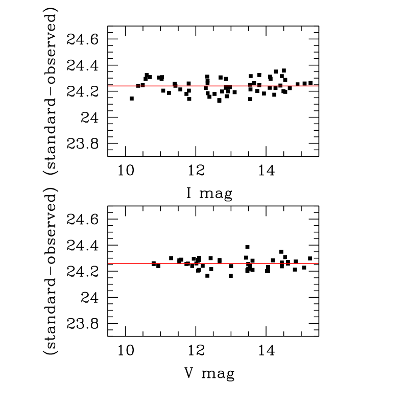
Figure 2: Standard star calibration plots for the $I$ and $V$ filters for the October 97 data (upper and lower panels respectively). For each panel, we plot the difference between the standard star magnitude and the instrumental magnitude (corrected to one airmass) as a function of the true $I,V$ magnitudes. The solid line shows the adopted zero-point; this is $24.24\pm 0.04$ ($V$) and $24.26\pm 0.06$ ($I$), per second and at one airmass. Atmospheric extinction coefficients are taken from the CFHT handbook, although most of our standards are at or near the zenith.

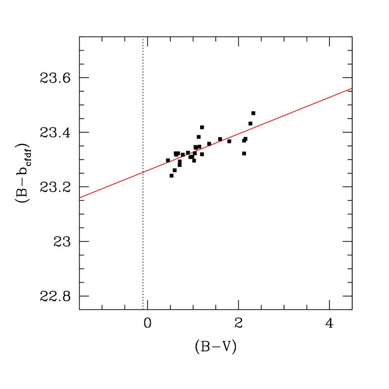
Figure 3: $B-b_{cfdf}$ vs $(B-V)$, based on observations of $51$ standard stars during the October 1997 observations. The slope and offset of the fitted line is 0.07 and 23.26, respectively. The slope is not well determined due to the small range in (B-V) colours spanned by our observations and we expect errors of $\sim 0.02$.

2.5 Systematic photometric errors

To measure accurately the galaxy clustering signal it is essential that the photometric zero-point is uniform across the stacked images. Zero-point variation across the mosaic will introduce excess power on large scales and contribute to a flattening of the $\omega(\theta)$ on large scales. For single-CCD images, improperly flattened data can produce this effect; in our case we have the additional complication that we must correctly account for the different responses and amplifier gains for the eight CCDs in our mosaic. As outlined above, this is accomplished by scaling each CCD image before co-addition to have the same sky background. Our standard star reductions detailed in Sect. 2.4 have already indicated that this procedure produces zero-point variations on order $0.05$ magnitudes r.m.s. . However, further observations allow a more rigorous test of this effect. On two separate occasions we have observed the same field (11hr, 22hr) after the camera bonnette had been rotated $180\deg$. These data provide an excellent opportunity to verify that there are no residual systematic magnitude zeropoint variations in our final stacks after co-addition and stacking have been carried out.

To carry out these tests we prepare two separate stacked mosaics. For the field at 11hrs, we have 4.4hrs of integration in I from December 1996 and 3hrs total integration from May 1997. By using sources extracted from the December run to compute our astrometric solution following methods outlined above, we can produce final stacked mosaics which are aligned with a standard deviation of $<1$ pixel over the entire field of view. By carrying out the detection process on the sum of these two images, and photometry on the two separate mosaics, we are able to measure the difference in magnitude between sources located in the same part of the sky but falling on different elements of the detector-telescope system. Note that because we place our photometric apertures on the same positions on each of the two stacks, this test also allows us to investigate magnitude errors introduced by mapping inaccuracies between the two stacks, which are expected to be present for the measurement of aperture colours.

The results of this test are illustrated in Fig. 4 where we plot the difference in magnitude for non-saturated stellar sources with $18.5<I_{AB}<22.5$ between the two 11hr stacks as a function of position in both $x$ and $y$ directions. We find that the systematic magnitude errors, measured as the dispersion of these residuals is $\sim 0.04$ magnitudes, which corresponds to the limit of our CCD-to-CCD calibrations, as explained in Sect. 2.4.

Towards the $50\%$ completeness limit of our catalogues, $I_{AB}\sim 25.5$, differential incompleteness becomes a significant bias in the measurement of $\omega(\theta)$. This effect arises from the differing read-out electronics and detector gains used in each of the eight individual CCDs in UH8K. Neuschaefer & Windhorst (1995), using the Palomar four-shooter camera, discuss this effect in more detail. However, we emphasise that all our scientific analysis is only carried out where our completeness is $>80\%$, as determined from the simulations and source counts detailed in the following sections. Furthermore have verified that this effect is only significant at the faintest magnitudes by adding 40,000 objects with the same clustering amplitude as galaxies at $I_{AB}\sim 25$ to one of our images. This test is described in detail in Sect. 5.2.

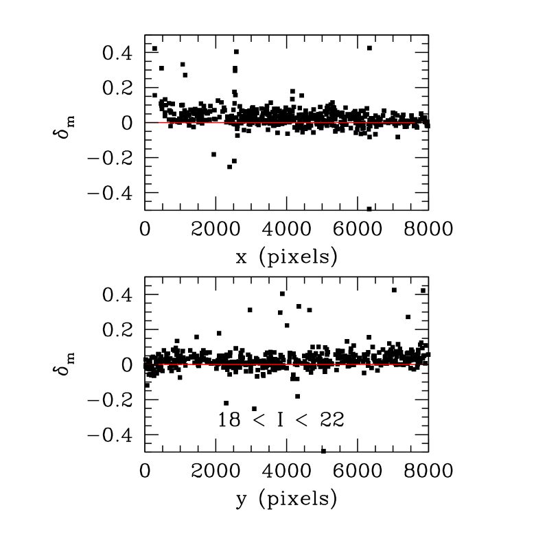
Figure 4: The magnitude difference as a function of $x$ and $y$ position between non-saturated stellar sources with $18.5<I_{AB}<22.5$ in the December 1996 11hr stack and the May 1997 data covering the same field. We find $\sigma(\delta_{m})\sim 0.04$ magnitudes.

2.6 Random photometric errors

We may also use these repeated observations of the same field to investigate what random photometric errors are present in our data. At fainter magnitudes these errors dominate. We have used three separate methods to estimate the magnitude errors computed in our data; firstly, we may use the errors computed directly by sextractor; secondly, we can use the errors computed from the simulations detailed in Sect. 2.7 in which stellar objects are added to our fields and recovered; and lastly, we may use the our two independent stacks of the same field to estimate our errors.

Fig. 5 shows magnitude errors for these three different estimators: sextractor (circles), the simulation (stars) and from the direct measurement (squares). We have carried out these tests on both the 11hr stacks and the 22hr stacks. In many magnitude ranges, the sextractor errors are lower than the other two measurements. We believe the origin of this discrepancy is due to the image resampling and interpolation process which produces images with correlated background noise. By contrast, the sextractor magnitude errors are computed assuming white background noise.

Figure 5: Root-mean-square (RMS) magnitude errors as a function of $I_{AB}$ magnitude. The upper and lower panels shows measurements made on the 11hr and 22hr fields respectively. Magnitude errors were computed using a variety of techniques: from sextractor (open circles); from a simulation in which stars were added to random patches of the field (stars) and the dispersion in the recovered total magnitudes is calculated; and finally as measured between two independent stacks covering the same field (open squares). The direct magnitude error measurements have been multiplied by $\sqrt{2}$ to account for the shorter exposure time for the individual stacks. At all magnitudes the sextractor errors appear to underestimate the both the direct and simulation error by at least a factor of two.

2.7 Incompleteness simulations and limiting magnitudes

In Table 1 we list the $3\sigma$ values for detection in a 3” aperture. These should be regarded as lower limits on the detectability of the galaxies in our catalogues. To better characterise the photometric properties of our images we have carried out an extensive set of simulations. These simulations involved adding artificial stars and galaxies to our single-band images and measuring the fraction recovered as a function of magnitude. In Fig. 6 we show the results of one set of such simulations for the 03hr field.

We note that this result should be regarded as lower limit to the completeness in our data as our actual catalogues are constructed using the chisquared technique described in Sect. 3.1 and can be expected to be slightly deeper (but note also that in constructing the chisquared catalogues all images must first be convolved to the worst seeing). From a rough comparison of the $I-$band galaxy counts presented in Fig. 9, we see that the we see that the simulations provide a good estimate of the magnitude at which the the observed counts begin to fall off.

Figure 6: Derived completeness in four bands for the 03hr field as a function of AB magnitudes. These simulations were derived by adding 1,000 artificial stars in each half-magnitude interval to the original images and measuring how many objects were recovered as a function of magnitude. The detection threshold used for this test (number of sigmas above the noise background and minimum number of connected pixels) were the same as used for the actual detections on the $\chi^{2}$ image.

2.8 Comparison with CFRS photometry

Three of our fields (22hr, 03hr, 14hr) cover the original survey fields of the Canada-France Redshift Survey (CFRS; Lilly et al. (1995)). For the 22hr and 14hr field we have $BVI$ photometry from the CFRS; for the 03hr field, data exists in the $VI$ bandpasses.

For all these fields we have carried out a detailed comparison of our photometry with CFRS photometry. In Fig. 7 we compare $V$ and $I$ photometry from our stacked images with the CFRS for $V$ and $I$ filters in the 03hr and 14hr fields. For the 14hr fields, the agreement with the CFRS photometry is $<0.1$ magnitudes or better. In the 03hr field, however, we find that our magnitudes are $\sim 0.2$ and $0.1$ magnitudes brighter than CFRS magnitudes in the $V$ and $I$ filters respectively. We suspect the origin of this discrepancy is that the CFRS fields were selected to have low galactic extinction as measured in the maps of Burstein & Heiles (1982) (BH). In Table 2 we show that the difference between the BH extinction and the more recent $E(B-V)$ values given in Schlegel et al. (1998) is non-negligible (amounting to $\sim 0.15$ in $I_{AB}$ magnitudes). In all our fields we apply extinction corrections based on $E(B-V)$ values from Schlegel et al. (1998).

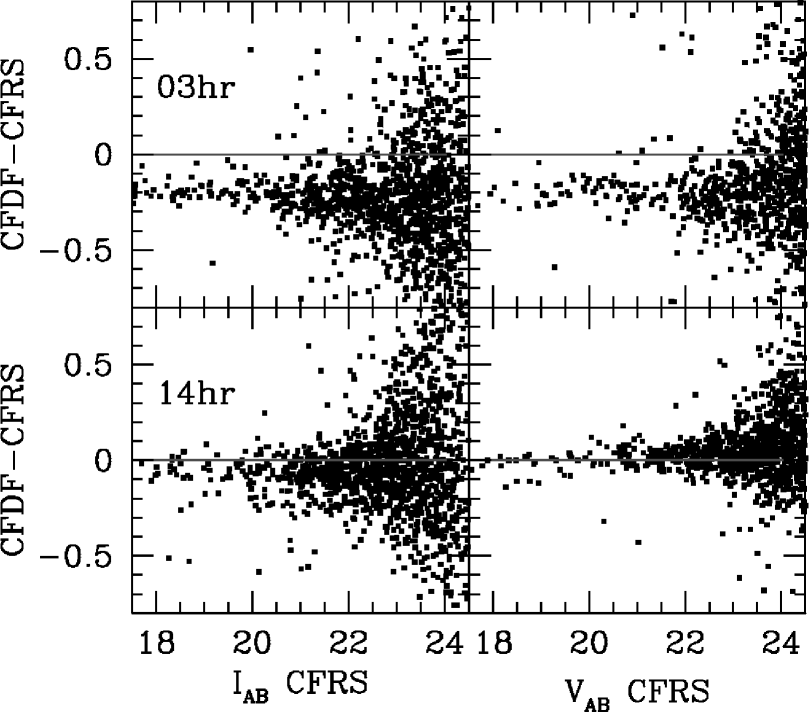
Figure 7: Comparison between CFDF and CFRS magnitudes measured in 3” aperture diameter for the $V$-band (right panels) and $I-$ band (left panels). The $\sim 0.2$ magnitude offset between CFRS and CFDF magnitudes for the 03hr field is a consequence of the significant galactic extinction in this field, which the CFRS magnitudes have not been corrected for.

3 Catalogue preparation

3.1 Construction of merged catalogues

To prepare merged catalogues with $UBVI$ colours for each object we derive a “detection” image to locate objects and then perform aperture photometry on each separate filter at the positions defined by the detection image. This procedure avoids the difficulties associated with merging separate single-band detection images (such as differences in object centroids between $U-$ and $I-$ band images, for example). This detection image is constructed using a $\chi^{2}$ image technique (Szalay et al., 1999), expressed in equation (2), where $a_{i}$ represents the background-subtracted pixel value in filter $i$, $\sigma_{i}$ the rms noise at this pixel and $n$ is the number of filter,

$$\chi^{2}={1\over n}\sum_{i=1}^{i=n}(a_{i}/\sigma_{i})^{2}.$$ (2)

This image has the advantage over other (more arbitrary) combinations of images such as $(V+I)$ in that it has a simple physical interpretation, namely that each pixel of this image represents the probability of detecting an object at that location. We compute $a_{i}$ and $\sigma_{i}$ for each pixel in each of the stacks using sextractor; this procedure allows us to correctly account for regions of varying signal-to-noise such as the overlap regions at the CCD boundaries. This resulting image is then used as input to sextractor as a detection image in the dual-image mode. We note that this method requires that both images are convolved to have the same full-width at half maximum and furthermore that they have a positional accuracy between filters of better than 1 pixel (as we have demonstrated in Sect. 2.3 our internal positional accuracy is $\sim 0.3$ pixels, which meets this objective). We use an empirical approach to set the detection threshold in the chisquared image, similar to that employed in da Costa et al. (1998). Based on the numbers of objects detected in “blank” images (frames which have the same background noise as our real images), the noise threshold is lowered in the chisquared image until the the number of additional sources detected is less than twice the number of sources detected in the blank images for the same change in the threshold. We emphasise however that the exact choice of the threshold is unimportant in this work as the range of variations considered in this procedure ($\sim 2.0\sigma$) does not affect object detection even at the faintest magnitude limit where we carry out our scientific analysis ($I_{AB}\sim 25$).

3.2 Effect of $\chi^{2}$-technique on galaxy magnitudes

As object parameters crucial to galaxy photometry, such as half-light radius, are extracted from the detection image when using sextractor in dual-image mode (in addition to the normal ($x$,$y$) centroids) we wished to ensure that the use of the $\chi^{2}$ image did not bias our derived (total) magnitudes. In Fig. 8 we plot the difference in galaxy total magnitudes between the single band 03hr image and the dual-image mode method ($\chi^{2}$ image and stacked image) as a function of total $AB$ magnitude in the single-band image. The filled shaded points show the median magnitude difference in half-magnitude intervals. Until $I_{AB}\sim 24$, $I_{AB}\leavevmode\nobreak\ (direct)-I_{AB}(\chi^{2})\lesssim 0.02$; for $24<I_{AB}<25.5$, $I_{AB}\leavevmode\nobreak\ (direct)-I_{AB}(\chi^{2})\lesssim 0.1$. Beyond $I_{AB}\sim 24$ magnitudes computed using the direct image become systematically brighter than the chisquared image, which is most likely a consequence of the more reliable object profile information contained in the chisquared image (which is comprised of effectively a sum of object fluxes over all filters). In any case our galaxy colour measurements, which use aperture magnitudes, are unaffected by the application of this technique.

Our final catalogues consist of matched $V,I$ band catalogues for all fields. For fields 14hr, 22hr and 03hr we have additional $B$ and $U$ band imaging. Magnitudes in our catalogues are Kron (Kron, 1980) “total” magnitudes computed using the sextractor $mag_{auto}$ parameter. We have also carried out a comparison between these magnitudes and those computed using the software employed in Le Fèvre et al. (1986) and the “Oxford” galaxy photometry package described in Metcalfe et al. (1991). We find no evidence of any systematic differences between these three softwares. Throughout this paper we measure colours in an aperture of $1.5^{\prime\prime}$ radius.

We also perform star-galaxy separation using the $r_{h}$ parameter from sextractor, which is carried out on the $I-$ band catalogue. This parameter measures the radius which encloses half the object flux. Star-galaxy separation is not carried out faintwards of $I_{AB}\sim 21.5$; in any case for high galactic latitude fields like ours galaxies outnumber stars by a large fraction at these faint magnitudes (Reid et al., 1996). The bright limit of our catalogue (above which all galaxies and stars are saturated) is $I_{AB}\sim 18.5$.

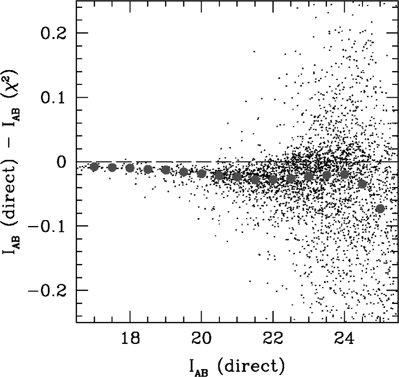
Figure 8: The difference between Kron (1980) total magnitudes computed in the direct 03hr $I-$band image and using the $\chi^{2}$ technique ($\chi^{2}$ detection image combined with $I-$ band photometry image) as a function of total magnitude measured in the $I-$band direct image (for clarity only 1/4 of all points are shown). The filled shaded points line shows the median difference in half magnitude intervals.

4 Galaxy counts and colours

4.1 $I_{AB}-$ and $B_{AB}-$ selected galaxy counts

In Fig. 9 and Fig. 10 we present $I-$ and $B-$band galaxy counts as a function of $AB$ magnitude derived from the CFDF survey (open thick circles) compared with the compilation of Metcalfe et al. (2000)(small points). For the $I-$ band we have four independent fields, or approximately $\sim 10^{5}$ galaxies; for the $B-$ band there are currently three fields with a total of $\sim 0.75\times 10^{5}$ sources. In both these filters we find an excellent agreement with the literature compilations extending over almost six orders of magnitude.

We find the fitted slope, $\alpha$, for $20<I_{AB}<24$ to be $0.35\pm 0.02$, which agrees quite well with the value quoted in Metcalfe et al. (2000) of 0.33 for the slightly deeper limits of $21<I_{kc}<25$. Note that all our $I-$data, from $I_{AB}\sim 18$ to $I_{AB}\sim 24$ (beyond which the effects of incompleteness begin to be important) is consistent with a constant slope in the number-magnitude relation.

We also compare our counts to those of Postman et al. (1998) (filled squares). This dataset is a $16\deg^{2}$ survey comprising $256$ separate exposures of $900s$ each. This dataset is $\sim 20\%$ below the CFDF faintwards of $I_{AB}\sim 22$ and remains so until the effects of incompleteness begin to dominate the CFDF counts. Furthermore, in our source counts we see no evidence of the inflection seen at $I_{AB}\sim 22$ in the Postman et al. counts.

For the $B-$counts we find a fitted slope in the range $20<B_{AB}<24$ of $0.47\pm 0.02$, consistent with the value of $0.50$ quoted in Brunner et al. (1999).

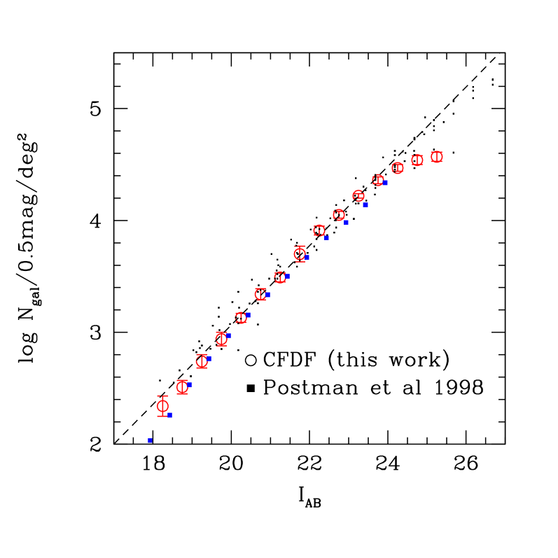
Figure 9: $I_{AB}-$ band galaxy counts for the four fields in the CFDF survey (open circles). The dashed line shows a least-squares fit to the bright data ($22<I_{AB}<24$). The error-bar on each point corresponds to the field-to-field variance. The filled squares show galaxy counts from Postman et al. (1998); the small points are from the compilation of Metcalfe et al. (2000).

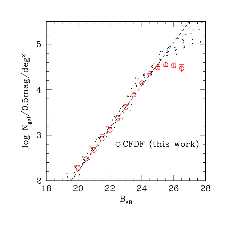
Figure 10: As in Fig. 9 but for the $B_{AB}$ selected galaxy counts.

4.2 Galaxy colours

In Fig. 11 we show $(V-I)_{AB}$ colours measured as a function of $I_{AB}$ total magnitude for galaxies in the CFDF 11hr field (for clarity only 1/8 of all galaxies have been shown). The dashed line represents the colour incompleteness computed using the limiting magnitudes given in Table 1. Our median $(V-I)_{AB}$ colours in half magnitude slices (filled circles) shows good agreement with colours derived from the NTT deep field (Arnouts et al., 1999b), shown as open squares, and this agreement continues to the completeness limit of our data.

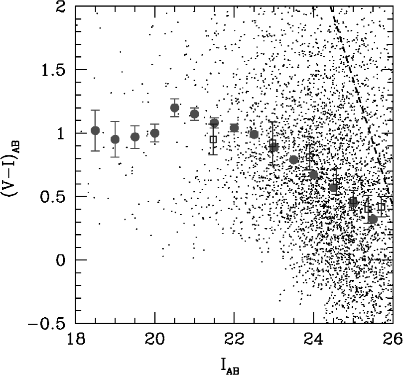
Figure 11: Median $(V-I)_{AB}$ galaxy colour, measured as a function of $I_{AB}$ total magnitude, for galaxies in the CFDF-11hr field (for clarity only 1/8 of all galaxies are shown). The filled circles show the median galaxy colour in half magnitude intervals; the open squares show the median $(V-I)_{AB}$ colours measured in the NTT deep field (Arnouts et al., 1999b). The dashed line shows the nominal colour incompleteness, based on the detection limits given in Table 1.

5 Measurements of $\omega(\theta)$ in the CFDF fields

5.1 Measuring $\omega(\theta)$

There is an extensive literature on the measurement of the projected galaxy correlation function in deep imaging data (Efstathiou et al., 1991; Roche et al., 1993; Brainerd et al., 1994; Hudon & Lilly, 1996; Woods & Fahlman, 1997; McCracken et al., 2000). Here we will only briefly outline the relevant equations. We have computed the two-point projected galaxy correlation function using the Landy & Szalay (1993) (LS) estimator,

$$\omega(\theta)={\mbox{DD}-2\mbox{DR}+\mbox{RR}\over\mbox{RR}},$$ (3)

with the $DD$, $DR$ and $RR$ terms referring to the number of data-data, data-random and random-random galaxy pairs between $\theta$ and $\theta+\delta\theta$. In this work we use logarithmically spaced bins with $\log(\delta\theta)=0.2$.

The fitted amplitudes quoted in this paper assume a power law slope for the galaxy correlation function, $\omega(\theta)=A_{\omega}\theta^{-\delta}$; however this amplitude must be adjusted for the “integral constraint” correction, arising from the need to estimate the mean density from the sample itself. This can be estimated as (Roche et al., 1993),

$$C={1\over{\Omega^{2}}}\int\int\omega(\theta)d\Omega_{1}d\Omega_{2},$$ (4)

where $\Omega$ is the area subtended by each of our survey fields. For the CFDF fields, we find $C\sim 4A_{\omega}$ by numerical integration of Equation 5 over our field geometry and assuming that galaxies closer than $1^{\prime\prime}$ cannot be distinguished. In deriving the correlation amplitudes we then fit

$$\omega_{obs}(\theta)=A_{\omega}\theta^{-\delta}-C,$$ (5)

where $\omega_{obs}(\theta)$ is our observed measurement of $\omega(\theta)$. (We note however that the integral constraint correction only becomes important at larger scales ($\theta>2\arcmin$) and that the large numbers of galaxies in our survey combined with the large field of view of each patch means we can fit for $A_{\omega}(1\arcmin)$ while neglecting the integral constraint, providing the range of the fit is restricted to scales where the integral constraint is not important). In our fitting procedure we use the method of Marquardt (1963) which takes into account that each measurement of $\omega(\theta)$ at each angular separation is not independent of the others.

To minimise computational requirements (necessary given the large numbers of galaxies in our samples, typically 30,000 galaxies per field) we use a sorted linked list method to compute the numbers of galaxy pairs in each angular bin (and furthermore we have verified that this method gives the same results as a direct-pair counting approach; it is, however $\sim 2-3\times$ faster). We use polygonal masks to blank out regions surrounding bright stars, large galaxies, satellite trails and cosmetic defects. We also discard data from CCD 8 because of its poor charge transfer properties. Our masking strategy is quite conservative, and (excluding CCD 8), around $15-20\%$ of the total area is removed. Because the 11hr and 22hr fields are composed of two separate stacks which are rotated relative to each other, are able to cover the entire $28^{\prime}\times 28^{\prime}$ area for these fields. We have verified that the masks do not bias the determination of $\omega(\theta)$ function by applying them to randomly generated catalogues with the same number density as the real catalogues and verifying that $\omega(\theta)$ is zero at all angular scales. We have also tested the effect of masks on clustered catalogues generated using the method of Soneira & Peebles (1978). These tests (which were carried out using the LS estimator) show that the application of masks does not change our fitted correlation amplitudes. Note that we do not apply a stellar dilution correction to our measured correlation amplitudes as some authors do, as the form of the stellar counts for high galactic latitude fields is not precisely known. However, this correction is unlikely to raise the amplitude of the correlation function by more than $10-15\%$, given that stars outnumber galaxies by at least an order of magnitude beyond $I_{AB}\sim 21.5$.

5.2 $\omega(\theta)$ for $I_{AB}$ magnitude-limited samples

For each of our four fields, we divide our catalogue into magnitude limited samples. Each sample reaches one half-magnitude deeper than the previous, while the bright limit is kept at $I_{AB}=18.5$. (As the 14hr field is shallower than the other fields, we do not measure $\omega(\theta)$ on this field fainter than $I_{AB}=24.0$). These samples are extracted from the $\chi^{2}$ catalogues prepared as outlined in Sect. 3.1; we have also performed the same computation on single-band catalogues (i.e, those computed without using an associated $\chi^{2}$ image for detection) and find identical results. Fig. 12 shows the logarithm of the amplitude of $\omega(\theta)$ averaged over the four fields of the CFDF as a function of the logarithm of the angular separation in degrees, for a number of magnitude-limited samples. In the range $-2.5<\log(\theta)<-1.3$ ($0.2^{\prime}<\theta<3^{\prime}$) our measurements follow the expected power-law behaviour very well and at least until $I_{AB}\sim 24$ there is no evidence of significant excess power on scales larger than the individual UH8K CCDs ($\sim 10^{\prime}$), in agreement with the evidence presented in Sect. 2.5 that the systematic photometric errors in our fields are negligible.

Figure 12: The logarithm of the average amplitude of the angular correlation function, $\omega(\theta)$, as a function of the logarithm of the angular separation in degrees, for all fields in the CFDF. The error bar on each bin is computed from the field-to-field variance. Each of the five different symbols shows a different magnitude-limited sample; the solid lines shows the fitted correlation amplitude. This weighted fit is carried out neglecting the three innermost bins and assuming a power-law slope of $-0.8$ for $\omega(\theta)$ and a value of $4.2$ for the integral constraint term $C$. Data from the 14hr field is not included in the faintest slice.

Figure 13: Simulated measurements of $\omega(\theta)$, (b,c), compared with CFDF measurements for slice $18.5<I_{AB}<24.0$, (a). In each case the simulated measurements have been normalised by the fitted amplitude for the $18.5<I_{AB}<24.0$ slice, taking into account the integral constraint correction and assuming a $\delta=-0.8$ power law. The simulations (b,c) contain objects in the magnitude range $23.5<I_{AB}<24.5$ and $24.5<I_{AB}<25.5$ respectively. Each plot has been offset by an arbitrary amount $x$ where $x=0,1.5,3.0$.

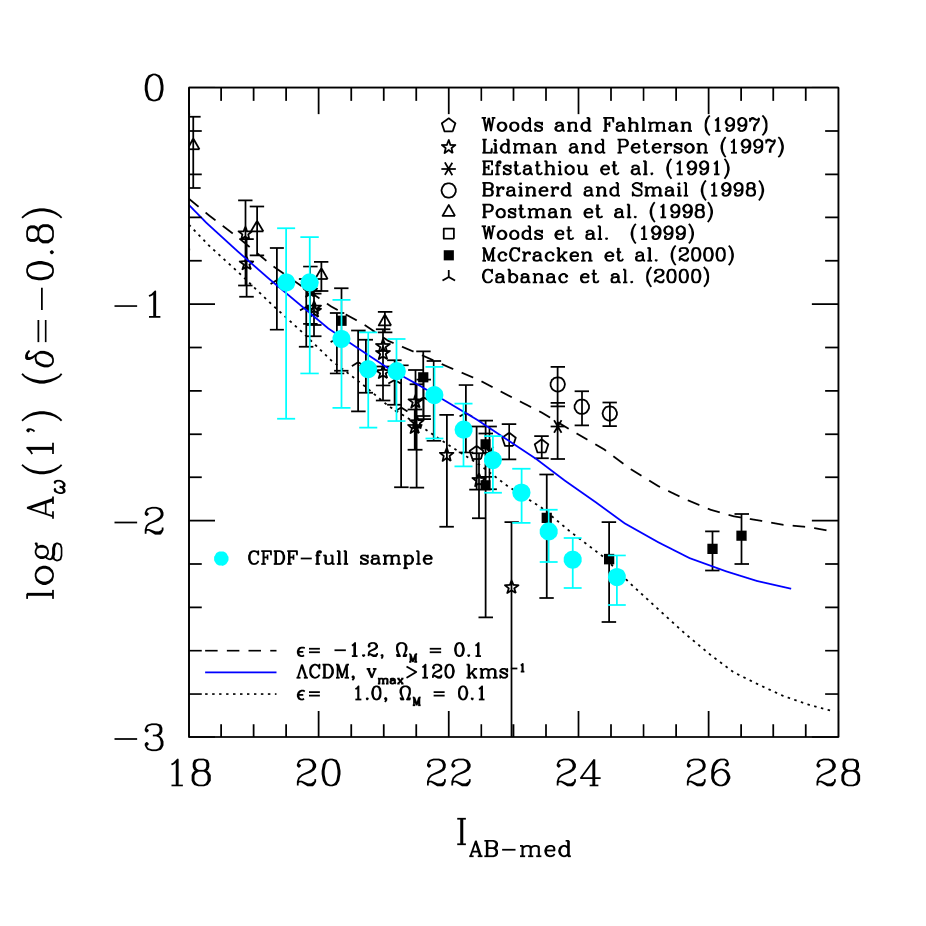
Figure 14: The logarithm of the fitted amplitude of the angular correlation $\omega(\theta)$ at $1^{\prime}$ as a function of sample median $I_{AB}$ magnitude (filled circles). Fits were computed assuming a power law of slope $\delta=-0.8$ for $\omega(\theta)$ and an integral constraint term calculated as described in the text. Error bars on the CFDF points are computed from the analytic expression of Bernstein (1994). The model curves are taken from McCracken et al. (2000) and show three different clustering evolution scenarios which are detailed in the text.

At $\theta<0.2^{\prime}$ we find at fainter magnitudes that $\omega(\theta)$ deviates from the expected power-law behaviour. We have attempted to investigate the origin of this effect (which is seen in all our fields) by carrying out an extensive set of simulations. In these simulations we generate a catalogue with $\sim 40,000$ objects which have the same correlation amplitude as the $I_{AB}\sim 24$ sample. Each of these objects is assigned a random magnitude in a specified interval and then added to the data frame. Object detection and photometry is carried out in a box extracted at this location. A new catalogue is constructed containing recovered total magnitudes for each object, and a magnitude cut is then applied to this sample. Objects which are lost in this process are typically those falling on or near bright stars or galaxies, or those whose recovered total magnitude falls outside our magnitude cut. Masks are applied to this catalogue and $\omega(\theta)$ computed using the same procedures used for the real data. This procedure is then repeated for progressively fainter magnitude slices. (In constructing the simulated catalogue, two simplifying assumptions were made, firstly that the input magnitude distribution of objects is flat, and secondly we use objects with Gaussian point-spread functions.)

In Fig. 13 we show the results of two of these simulations, labelled (b) and (c). The results displayed for (a) show the measured correlations for the $18.5<I_{AB}<24.0$ magnitude slice. In order to display deviations from the power-law behaviour, each slice has been normalised by the fitted amplitude for the $18.5<I_{AB}<24.0$ slice, taking into account the integral constraint correction and assuming a $\delta=-0.8$ power law. These simulations cannot reproduce the depression in the correlation function found at scales $\log(\theta)\sim-2.5$. We have also investigated if the depression is caused by an excess of objects around bright stars, and have found no evidence of such an excess. An important aspect of these simulations, however, is that they confirm that excess power on large scales only becomes important for the CFDF data for the faintest magnitude ranges, $24.5<I_{AB}<25.5$.

In Fig. 14 we plot the fitted amplitude of $\omega(\theta)$ at one arcminute, $A_{\omega}(1\arcmin)$, averaged over all our fields, (filled circles) as a function of the sample median AB magnitude ($I_{AB-med}$). We have estimated the error bars on $A_{\omega}$, $\delta A_{\omega}$, using an analytic approximation introduced by Bernstein (1994) and further developed by Szapudi & Colombi (1996); see also Arnouts et al., in preparation. for a detailed explanation of the application of this approximation. The Bernstein estimator relies on a knowledge of the higher-order moments of the galaxy correlation function, $S_{3}$ and $S_{4}$; we have estimated these quantities directly from the CFDF dataset and they will be presented in a future work (Colombi et al., in preparation). At bright magnitudes ($I_{AB-med}\sim 18$), $\delta A_{\omega}$ is dominated by the Poisson error component; however, faintwards of $I_{AB-med}\sim 22$, the main component of $\delta A_{\omega}$ in our field consists of cosmic variance (or “finite volume”) effects. Our analytic estimates of this effect indicate that the errors estimated empirically from the field-to-field variance of our four fields may underestimate the total error at these magnitudes by around $\sim 20\%$.

Our fitted amplitudes were computed assuming a $-0.8$ slope for $\omega(\theta)$ (to allow a comparison with the literature), and over the range $0.2^{\prime}<\theta<3^{\prime}$. We have also attempted to fit for $A_{\omega}$ only at larger separations ($\sim 3\arcmin$), but our survey fields are not large enough to detect any scale-dependence in the $A_{\omega}-I_{AB-med}$ relation. Additionally, Fig. 14 shows a compilation of recent measurements of $A_{\omega}$ from the literature. These literature measurements all assume a fixed slope of $\delta=-0.8$, with the exception of the Postman et al. survey, in which the slope was allowed to vary with the fit. To allow a fair comparison with the other authors, and with our work, the Postman et al. points are not plotted faintwards of $I_{AB-med}\sim 21$, where their fitted slopes begin to differ significantly from $-0.8$.

At bright magnitudes ($19<I_{AB-med}<22$) we find that our observations are compatible with almost all the data from the literature compilation. At fainter magnitude ranges, ($22<I_{AB-med}<24$), our observations clearly favour a low amplitude for $A_{\omega}$. At $I_{AB}\sim 24$ they are least a factor of ten below the value of $A_{\omega}$ found by Brainerd & Smail (1998). This work covers a small area ($\sim 50$ arcmin²) and consists of individual unconnected pointings. As has been suggested before (McCracken et al., 2000) the discrepancy may be due to field-to-field variance in the galaxy clustering signal. To provide a more direct answer this question, we extract 200 regions of $50$ arcmin² from the 22hr and 11hr fields (these two have complete coverage as a consequence of bonette rotations). On each of these sub-regions we measure $A_{\omega}$ as for the full sample. In Fig. 15 we show the histogram of the fitted values for the 11hr and 22hr fields; from this we estimate that a $\pm 3\sigma$ error bar indicates a dispersion of $\times 10$ in $A_{\omega}$. It is clear that the error bars on Brainerd & Smail measurement underestimate the true error by a large amount.

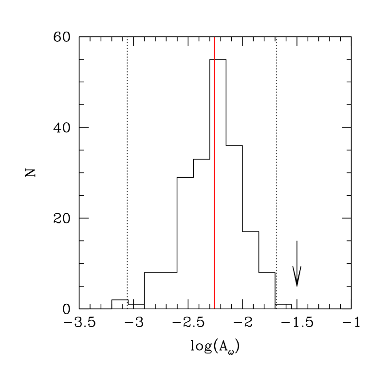
Figure 15: The logarithm of the fitted correlation amplitude at $1\arcmin$, $\log(A_{\omega})$ measured on 200 $7\arcmin\times 7\arcmin$ sub-areas extracted from the 11hr and 22hr fields. Galaxies extracted have magnitudes in the range $18.5<I_{AB}<25.5$. The dotted lines represent $\pm 3\sigma$ confidence limits about the mean value, shown by the solid line. The arrow shows approximately the $A_{\omega}(1\arcmin)$ measured by Brainerd & Smail (1998).

We have also determined $A_{\omega}(1\arcmin)$ in one-magnitude slices, for instance, $19.5<I_{AB}<20.5$, $20.5<I_{AB}<21.5$ to the limit of our survey, as an additional check. These measurements are considerably more noisy than the integrated measurements presented above because of the smaller numbers of galaxies in each slice. However, we find that the derived $I_{AB-med}-\log A_{\omega}(1\arcmin)$ relation is very similar to what is presented in Fig. 14.

5.3 Dependence of slope on magnitude

The large numbers of galaxies in our survey allows us to make a direct measurement of $\delta$, the slope of $\omega(\theta)$ as a function of sample limiting magnitude. Several attempts at this measurement have been carried out but with generally inconclusive results. Neuschaefer & Windhorst (1995) find $\delta=-0.5$ at $g<25$ based on two independent fields each the size of one of our CFDF fields. Shallower wide-angle surveys like those of Roche & Eales (1999) and Cabanac et al. (2000) find no evidence for deviation from a slope of $\sim 0.8$. One difficulty in this measurement is that excess power on large scales, such as can be produced by zero-point variations, can produce an artificially shallow slope. However, we have already demonstrated that our magnitude zero-point errors are small across our mosaics (Fig. 4) and that differential incompleteness only becomes significant for measurements of $\omega(\theta)$ in the CFDF fields at very faint magnitudes (Fig. 13). Nevertheless, we adopt a cautious approach and use two different methods to measure $\delta$.

Firstly we compute $\chi^{2}$ contours from the average correlation per angular bin over all the fields (Fig. 12), shown in Fig. 16. In our second method we compute the slope independently for each field and measure the field-to-field standard deviation of this fit, which is shown in Fig. 17, together with a comparison with the fitted slopes from Postman et al. (1998), computed for a fitting range of $0.5\arcmin<\theta<5\arcmin$. An additional complication is that in both cases our slope-fitting procedure requires an estimation of the integral constraint (Equation 5), which in turn depends on the slope. To limit these difficulties, we perform the fit only in the range $-0.2\arcmin<\theta<1.9\arcmin$ where the effects of the integral constraint are expected to be negligible.

Both methods indicate that at bright magnitudes, $18.5<I_{AB}<22.0$, $\delta\sim-0.8$; at fainter magnitudes we detect a slight flattening of the slope, with $\delta\sim-0.6$. The error bars in Fig. 17 show the error in $\delta$ for a given value of $A_{\omega}$; from Fig. 16 we see, however, that a slope of $\delta=-0.8$ is still within $3\sigma$ of our best fit for all magnitude ranges.

Figure 16: $\chi^{2}$ contours showing best-fitting amplitudes and slopes (plus symbols) for the four faintest CFDF samples, from right to left, $18.5<I_{AB}<22,23,24,25$. The three contours show the $1\sigma$ (thick contour), $2\sigma$ and $3\sigma$ confidence levels.

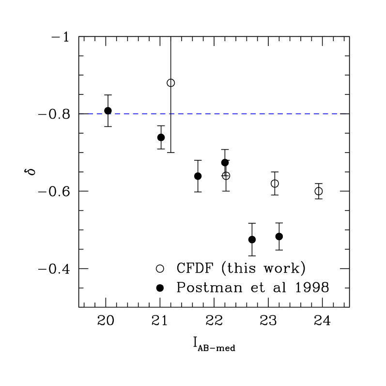
Figure 17: The fitted slope of $\omega(\theta)$ as a function of sample median magnitude (open circles) for galaxies with $18.5<I_{AB}<22,23,24,25$ averaged over the CFDF fields. Points are also shown from Postman et al 1998 (filled circles). Error bars on the CFDF points are computed from the variance over our four survey fields.

5.4 Galaxy clustering as a function of colour

For all galaxies in our sample we can measure $(V-I)_{AB}$ colours and we can use this to select subsamples by colour. In Fig. 18 we show $\log A_{\omega}(1\arcmin)$ as a function of $(V-I)_{AB}$ colour for galaxies with $18.5<I_{AB}<24.0$ (open pentagons) and $18.5<I_{AB}<23.0$ (asterisks). For each of the four fields, we divide our sample into twelve equally spaced bins in colour each of width $0.25$ in $(V-I)_{AB}$. The error bars in $\log A_{\omega}(1\arcmin)$ were computed from the field-to-field variance. Also shown as the dotted and dashed lines is the amplitude of $\log A_{\omega}(1\arcmin)$ for the full-field sample for these two slices.

We first note that both these cuts are relatively bright; at $I_{AB}\sim 24$ our catalogues are expected to be $\sim 100\%$ complete (Figs. 6, 9). Additionally, as shown in Fig. 11, the effect of colour incompleteness should be minimal, although at $I_{AB}\sim 24$ we may begin to lose some extremely red objects from our sample.

Our measurements clearly show that redder objects are more strongly clustered, as has been widely reported for local populations (Loveday et al., 1995). We find that objects with $(V-I)_{AB}\sim 3$ have a clustering amplitude at least a factor of ten higher than the full field population, shown as the dotted and dashed lines in Fig. 18. Interestingly, we also find that the bluest objects in our survey, those with $(V-I)_{AB}\sim 0$, have a clustering amplitudes marginally higher than the full sample. Furthermore, we find that none of our colour selected samples have clustering amplitudes below the full-field value. We discuss the implications of these results in the following section.

Figure 18: The logarithm of the fitted amplitude of the angular correlation $\omega(\theta)$ at $1^{\prime}$ as a function of sample median $I_{AB}$ magnitude (as before, fits assume $\delta=-0.8$). $\log(A_{\omega})(1\arcmin)$ was computed for 12 equally spaced bins of $0.25$ in $(V-I)_{AB}$. Error bars for each colour slice are computed from the field-to-field variance. Two magnitude ranges are shown, $18.5<I_{AB}<24.0$ (open pentagons) and $18.5<I_{AB}<23.0$ (asterisks), together with the fitted amplitude for the full field samples, dotted and dashed lines respectively.

6 Discussion and comparison with model predictions

6.1 Modelling $A_{\omega}$

For $r<20h^{-1}$ Mpc, the spatial correlation function $\xi(r)$ can be approximated by $\xi(r)=(r_{0}/r)^{\gamma}$, where, from the results of local redshift surveys, $\gamma\sim-1.8$ and $r_{0}\sim 4.3h^{-1}$Mpc (Groth & Peebles, 1977; Davis & Peebles, 1983; Maddox et al., 1990). One way to produce a prediction for the variation of $A_{\omega}$ with sample limiting magnitude is to assume a functional form for the growth of clustering $\xi(r,z)$, normally written as

$$\xi(r,z)=h(z)\left({r_{0}\over r}\right)^{\gamma},$$ (6)

where

$$h(z)=(1+z)^{-(3+\epsilon)}.$$ (7)

This functional form is then integrated over redshift space using the relativistic version of Limber’s equation, (Phillipps et al., 1978; Groth & Peebles, 1977; Limber, 1953), assuming that for $\theta\ll 1$ (Efstathiou et al., 1991),

$$\omega(\theta)=\sqrt{\pi}{\Gamma[(\gamma-1)/2]\over{\Gamma(\gamma/2)}}{A\over{\theta^{\gamma-1}}}r_{0}^{\gamma},$$ (8)

where $\Gamma$ is the incomplete gamma function, $\theta$ is the angular separation and $A$ is given by

$$A=\int^{\infty}_{0}g(z)\left(dN\over{dz}\right)^{2}dz/\left[\int^{\infty}_{0}\left({dN\over{dz}}\right)dz\right]^{2},$$ (9)

with

$$g(z)={h(z)\over{d_{A}^{\gamma-1}(z)}}\left({dr(z)\over{dz}}\right)^{-1},$$ (10)

where $d_{A}(z)$ is the angular diameter distance and $dr(z)/dz$ is the derivative of the proper distance. In this simple scenario, three cases are of interest: clustering fixed in proper coordinates, in which $\epsilon=0.0$; clustering fixed in co-moving coordinates which gives $\epsilon=-1.2$. Finally, the predictions of linear theory give $\epsilon=0.8$.

Many papers have investigated the scaling of $A_{\omega}$ with magnitude using the approach detailed above (see, for example, Efstathiou et al. (1991)). To interpret measurements of $A_{\omega}$, using these models, however, involves making at least two critical assumptions: firstly, the form of the redshift distribution $dN/dz$ for the faint galaxy population and its evolution as a function of limiting magnitude; and secondly how $\xi(r,z)$ scales with redshift (Equation 7). In the following section we examine these two assumptions in turn. (Predicted correlation amplitudes using this formalism are also sensitive to the underlying cosmology, as the size of the volume element at a given redshift is much lower for an Einstein-deSitter cosmology than for a low-$\Omega$ universe. However, to the median redshift of our survey the difference in model predictions between open and flat-Lambda cosmologies small. In this paper we assume that $\Omega_{M}\sim 0.1$, in agreement with recent observational evidence.)

6.2 Validity of model assumptions

Our $dN/dz$ is derived from luminosity evolution models which are described fully in Metcalfe et al. (2000). Starting with the observed local galaxy luminosity function and assuming a star-formation history for each galaxy type these models are able to reproduce the observed numbers counts, colours and redshift distributions of the faint galaxy population to the limits of the current observations (Metcalfe et al., 2000). However, at $I_{AB}\sim 24$ we may now directly test these model redshift predictions against spectroscopic measurements made in the Hubble Deep Field (HDF) (Cohen et al., 2000; Williams et al., 1996). In Fig. 19 (upper panel) we show the spectroscopic redshift distribution for 120 galaxies in the HDF-North (with 16 non-detections represented as the open box) compared to the predictions of our $\Omega_{M}=0.1,\Omega_{\Lambda}=0.0$ PLE model distribution (solid line). In the lower panel we show the relationship between median redshift $z_{med}$ and $I_{AB}$ limiting magnitude as predicted by this model (note that we compute our median redshift in each case by considering all galaxies brighter than the abscissa magnitude). Additionally, we show measurements from several other $I_{AB}-$ magnitude limited redshift surveys, including the HDF sample used in the top panel. We also show the median redshift derived from photometric redshifts for two samples limited at $I_{AB}<25$ for the HDF N/S, kindly supplied to us by S. Arnouts. The Poissonian error bars computed from all surveys are smaller than the symbols and are not plotted. The true field-to-field variance may of course be much larger, but the fact that we measure the same median redshift for both HDF-N/S catalogues suggest that it is not.

Despite these qualifying remarks, we conclude that our luminosity evolution models provide an acceptable fit to the observed redshift distributions at least to the depth to which we measure galaxy clustering in the CFDF photometric catalogues ($I_{AB-med}\sim 24$, or equivalently $I_{AB}\sim 24.5$). They are able to reproduce both the trend of $z_{med}$ with $I_{AB}$ and the dispersion in redshift at a given magnitude slice. Furthermore, as demonstrated in Metcalfe et al., they also correctly predict the numbers of $2<z<3$ galaxies. We therefore conclude that our modelling of $dN/dz$ is not a major source of uncertainty in our prediction of $A_{\omega}$.

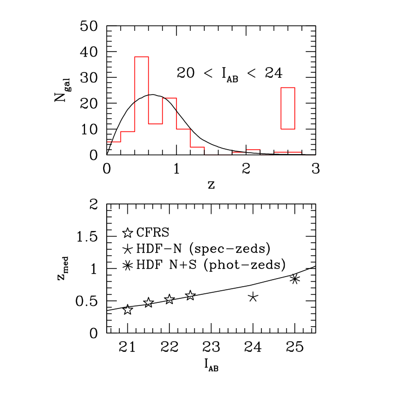
Figure 19: Upper panel: the redshift distribution of faint galaxies in the Hubble Deep Field North from the compilation of Cohen et al. (2000) (histogram), compared to the predictions of our model (smooth solid line). The open box represents the number of galaxies observed for which no redshift could be determined. Lower panel: the relationship between median redshift $z_{med}$ predicted by our model (solid line) compared to the CFRS (five-pointed stars), spectroscopic redshifts in the HDF-N (cross) and photometric redshifts from the HDF N/S (asterisk). Poissonian error bars are smaller than the symbols in all cases and are not plotted.

Our second assumption, that the growth of galaxy clustering can be expressed as in Equation (7), is more problematic. Clustering measurements of Lyman-break galaxies (Adelberger et al., 1998; Giavalisco et al., 1998), have already indicated that the “epsilon” formalism does not provide an acceptable fit to the observations . Similar results have also been found for measurements of $r_{0}(z)$ in the HDF-North (Arnouts et al., 1999a). Can our clustering measurements in the CFDF be successfully matched by this model? In Fig. 20 we show our measurements of $A_{\omega}(1\arcmin$) compared to prediction of our models for $\epsilon=-1.2,0.0,1.0,2.0$ (long dashed, solid, dotted and dashed lines respectively), assuming $r_{0}=4.3h^{-1}$ Mpc, $\Omega_{M}=0.1,\Omega_{\Lambda}=0.0$ and $\delta=-0.8$. (We note that clustering predictions for an $\Omega-\Lambda$ cosmology are very similar to zero-$\Lambda$ cosmology). For clarity we omit the literature compilation shown previously. In the magnitude range $18.5<I_{AB-med}<22$, we see that our observations are consistent with $\epsilon\sim 0$. However, faintwards of $I_{AB}\sim 22$, our observed clustering amplitudes decline more rapidly than the model predictions. By $23.0<I_{AB}<24.0$ our observations are consistent with $\epsilon\gtrsim 1$. From Fig. 20 it is clear that the $\epsilon\sim 0$ model cannot match simultaneously both bright and faint observations in the range $18.5<I_{AB-med}<24.0$. Furthermore, rapid growth of clustering for the entire sample ($\epsilon\sim 2$) is marginally excluded because it produces correlations which are already too low by $I_{AB-med}\sim 22$ to match our observations. Furthermore, allowing $r_{0}$ (i.e., $r_{0}(z=0)$) to vary merely changes the normalisation at $I_{AB}\sim 18.5$ (which is already in agreement with our observations) but not the slope of the $A_{\omega}(1\arcmin)-I_{AB-med}$ relation. In Sect. 6.4 we investigate the reason for this discrepancy in more detail.

6.3 Colour selected galaxy clustering

In Fig. 18 we clearly see the dependence of $\log(A_{\omega})$ on $(V-I)_{AB}$ colour. To interpret this result, we first note that the dependence of $(V-I)_{AB}$ colour on redshift and morphological type is well established, thanks to extensive spectroscopic surveys (Lin et al., 1999; Cowie et al., 1996; Crampton et al., 1995; Lilly et al., 1995). In particular, Wilson et al. (2001), using a large spectroscopic sample, demonstrated that objects with $(V-I)_{AB}\sim 3$ are predominately massive elliptical galaxies at $z\sim 0.8$. Furthermore, clustering amplitudes have recently been measured for objects selected to have extremely red colours in optical-infrared bandpasses (Daddi et al., 2000). These objects have clustering amplitudes $\sim 10\times$ higher than the full field population. It is probable that these objects are closely related to our $(V-I)_{AB}\sim 3$ sample; for galaxies with $(V-I)_{AB}>3$ at $I_{AB}<23.0$, we find $\sim 0.3$ N_gal arcmin^-2. In Daddi et al. (2000) using a selection of $(R-K_{s})>5.0$ and the slightly brighter limit of $K_{s}<19.0$, they find a surface density of $0.5$ N_gal arcmin^-2. The difference between our full field clustering amplitude at $18.0<I_{AB}<23$ and the clustering of objects selected with $(V-I)_{AB}\sim 3$ is approximately the same as the difference found by Daddi et al. between their $K_{s}$-selected sample and those of their extremely red objects.

Intriguingly, at the blue end of our selection, $(V-I)_{AB}\sim 0$, we also find a higher clustering amplitude than the full field sample, although the error bars are large due to field-to-field variations (at the $\sim 0.1$ magnitude level) in galaxy colours and the small numbers of objects involved. We have repeated our measurement of $A_{\omega}(1\arcmin)$ using an integrated selection (i.e., considering only objects redder or bluer than a specified colour cut) and find a similar effect. There is some evidence for this effect in the literature: working with photographic data, and considering objects in a somewhat brighter blue selected magnitude cut, $20<B_{J}<23.5$, Landy et al. (1996) also found an enhancement of at least $\sim 10$ for the clustering amplitudes of the bluest objects in ($U-R_{F}$).

Although Lyman-break galaxies are expected to be flat spectrum objects and therefore have $(V-I)_{AB}$ colours of $\sim 0$ their surface densities are not large enough to produce the effect seen in Fig. 18. The most likely explanation of this result is that these objects constitute a low-redshift population whose higher correlation amplitudes are a consequence of the lack of projection effects which dilute the measured $A_{\omega}$’s. Some evidence for this can been seen in Fig. 5. of Crampton et al. (1995); all objects with $(V-I)_{AB}\sim 0$ are at $z<0.3$. We also note that our red and blue samples have very low cross-correlation amplitudes, which supports the notion that the objects in our survey with $(V-I)_{AB}\sim 3$ and $(V-I)_{AB}\sim 0$ are separate populations at different redshifts.

6.4 Biasing and the growth of galaxy clustering

Given that the redshift distribution used in our models is in agreement with our observations, then it is clear that the discrepancy evident in Fig. 20 between model predictions and observations must be a result of evolution in the intrinsic properties of the galaxy population. Our simple model does not take this into account. As a first step towards a more realistic description of the data, we may try changing the form of the $r_{0}-z$ relation: McCracken et al. (2000), considered such a modification by adopting the form of $\xi(r,z)$ derived from dark matter haloes with $v_{max}>120$ kms^-1 identified in a large, high-resolution $N-$body simulation (Kravtsov & Klypin, 1999). This is shown as the solid line in Fig. 14. However, because the form of this relationship is very similar to the traditional “epsilon-model” in the range $0<z<1$, and because there are few $z>3$ galaxies in samples limited at $I_{AB}<25$, the differences in predicted amplitudes between this and the conventional formalism are small in the magnitude ranges we consider.

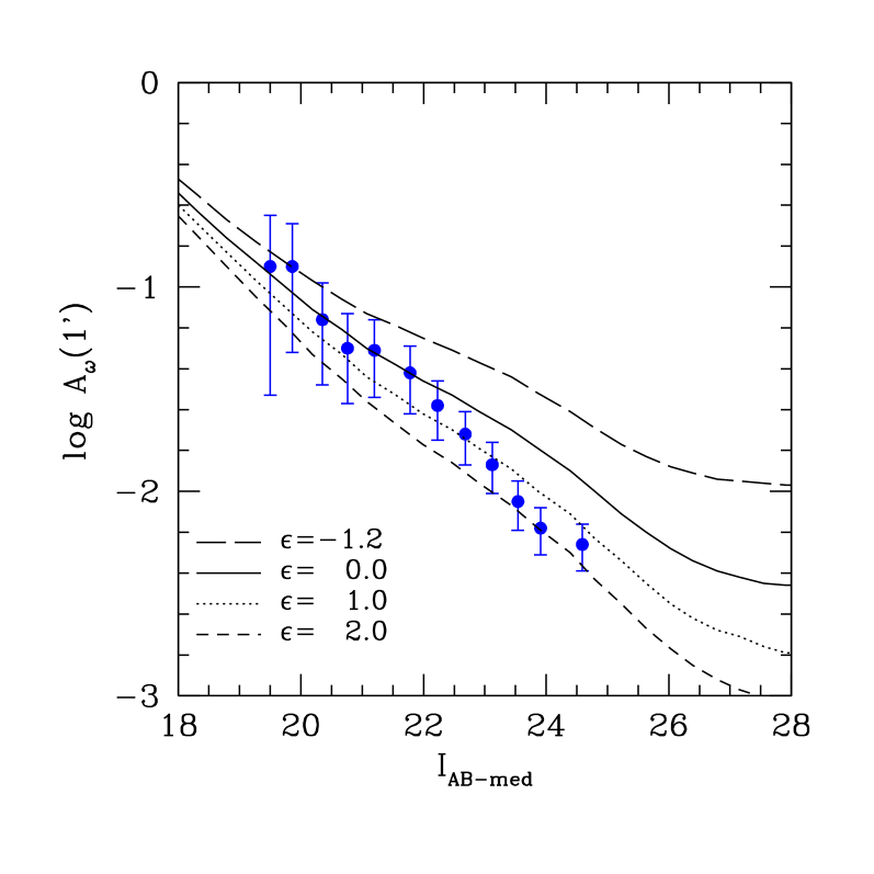
Figure 20: The evolution of $\log(A_{\omega}(1\arcmin))$ (assuming $\delta=-0.8,\Omega_{M}=0.1$ and $r_{0}=4.3h^{-1}$Mpc) for $\epsilon=-1.2,0.0,1.0,2.0$ (long dashed, solid, dotted, and dashed lines respectively). The filled points show the CFDF full sample. This plot is similar to Fig.. 14 except the literature compilation has been omitted for clarity.

The basic reason why the “$\epsilon$”-models fail to reproduce the clustering of Lyman-break galaxies and the observed form of $r_{0}(z)$ at high redshift is that they implicitly ignore the existence of bias and that how galaxies trace the underlying dark matter depends on the mass of the dark matter halo (Kaiser, 1984; Bardeen et al., 1986). Measurements of galaxy clustering in semi-analytic models, which provide a prescription for how galaxies trace mass, show clearly that more luminous galaxies have clustering amplitudes very different from less luminous ones (Benson et al., 2001; Baugh et al., 1999; Kauffmann et al., 1999).

Furthermore, it is now reasonably well established from observations that locally the galaxy correlation length $r_{0}$ depends on morphological type and colour (Tucker et al., 1997; Loveday et al., 1995; Davis & Geller, 1976), and some evidence exists for a direct dependence between luminosity and clustering amplitude (Benoist et al., 1996). There are also indications that these trends continue to higher redshifts (Carlberg et al., 2000; Le Fèvre et al., 1996). Furthermore, in our dataset, the median field galaxy $(V-I)_{AB}$ colour changes by $\sim 0.4$ mag in the range $22<I_{AB}<24$ (Fig. 11); from Fig. 18 we see that changes in colour of this magnitude cannot produce the changes in amplitude of $A_{\omega}(1\arcmin)$ seen in the data. For this reason we suggest that the rapid decline in $A_{\omega}(1\arcmin)$ in the range $22<I_{AB-med}<24$ is a consequence of luminosity-dependent clustering segregation.

Extensive imaging and spectroscopic observations have demonstrated that, for any magnitude limited sample, as we probe to fainter magnitudes, the mean intrinsic luminosity of the field galaxy population becomes progressively fainter. This is illustrated in Fig. 21 where we show the absolute luminosity as a function of apparent magnitude for galaxies in the CFRS survey (Lilly et al., 1995) (open circles) and for galaxies in the HDF-North computed using photometric redshifts from the photometric catalogue of Fernández-Soto et al. (1999). For both these catalogues we also show the median absolute magnitudes computed in half-magnitude intervals of apparent magnitudes (open and filled circles for the CFRS and HDF respectively). We also include an estimate of the median differential luminosities $dL/dm$ from our luminosity evolution models (solid line). We see that between $I_{AB}\sim 20$ and $I_{AB}\sim 22$, within the CFRS sample, the median galaxy luminosity declines by $\sim 0.5$ magnitudes. In the range $22<I_{AB}<24$ we measure a decline of a further magnitude, although the uncertainties in the absolute luminosities computed from photometric redshifts in the HDF is probably at least $\sim 0.5$ magnitudes. The decline in model luminosities seen in the range $18.5<I_{AB}<22.5$ are a consequence of the steep faint-end slope we adopt for the spiral galaxy luminosity function. These faint galaxies at $I\sim 22$ are predominately late-type galaxies, as has been demonstrated by spectral and morphological classification (Brinchmann et al., 1998; Driver et al., 1998).

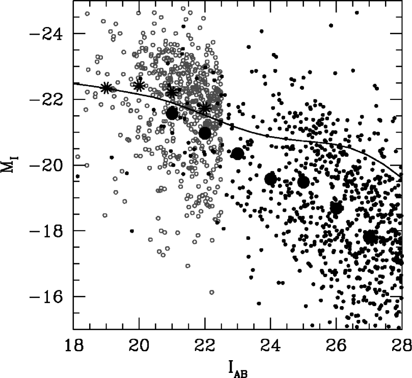
Figure 21: Absolute $I_{AB}$ magnitudes ($M_{I}$) and median absolute luminosities as a function of $I_{AB}$ magnitudes for galaxies selected from the CFRS (open circles, stars) and from the HDF-N (small and large filled circles). Model predictions of our luminosity evolution model are shown as the solid line (In all cases luminosities are computed assuming $h=0.5$ and an open $\Omega_{M}=0.1$ cosmology).

7 Conclusions

In this paper we have introduced a new wide-field deep imaging survey, the Canada-France deep fields project. Our survey covers a total area of $\sim 1$ deg² in four separate contiguous $0.25$ deg² fields. We have demonstrated that our reduction procedures are robust. Our internal astrometric errors are $\sim 0.06^{\prime\prime}$ and our systematic photometric errors across each $0.25$ deg² field are $\lesssim 0.04$ magnitudes.

In each of our four fields our galaxy catalogue is $\sim 100\%$ complete for $18.5<I_{AB}<24.0$. We find that in this range the $I_{AB}$ number-magnitude relation is well fitted by a line of constant slope $d\log(N)/dm\sim 0.35\pm 0.02$ in agreement with the literature compilations. Our completeness drops to $50\%$ at $I_{AB}\sim 25.5$.

Using this survey we have measured the projected-two point correlation function $\omega(\theta)$ for a sample of 100,000 galaxies as a function of sample median magnitude, $I_{AB-med}$, angular separation $\theta$ and $(V-I)_{AB}$ colour to $I_{AB-med}\sim 25.0$. At $I_{AB-med}\sim 24$ we measure the amplitude of $\omega(\theta)$ at $1\arcmin$, $A_{\omega}(1\arcmin)$ to an accuracy of $30\%$. Our conclusions are as follows:

1. We find that in the range $19.5<I_{AB-med}<24.0$, $A_{\omega}$ declines monotonically with sample limiting magnitude and that throughout this range, $\omega(\theta)$ is well matched with a power-law of slope $\delta$ for $0.2\arcmin<\theta<3.0\arcmin$. At bright magnitudes, $\delta\sim-0.8$; at $I_{AB-med}\sim 23$, we find $\delta\sim 0.6$, although our observations are still compatible with $\delta\sim-0.8$ at a $3\sigma$ confidence level.

2. We find a clear dependence of $A_{\omega}(1\arcmin)$ on $(V-I)_{AB}$ colour for galaxies selected in two magnitude ranges, $18.5<I_{AB}<24.0$ and $18.5<I_{AB}<23.0$. Galaxies with $(V-I)_{AB}\sim 3$ have clustering amplitudes $\sim 10$ times higher than the full field population. These objects are most probably evolved ellipticals at $z\sim 1$. We also find some evidence (at the $\sim 1\sigma-2\sigma$ level) for slightly higher clustering amplitudes for the blue $(V-I)_{AB}\sim 0$ objects in our sample.

3. We discuss model predictions and current spectroscopic determinations of the redshift distribution $dN/dz$ for the faint field galaxy population. We conclude that for $19.5<I_{AB-med}<24.0$, $dN/dz$ is now well determined. Using these predictions we find that for low $\Omega$ cosmologies, and assuming a local galaxy correlation length $r_{0}=4.3h^{-1}$Mpc, the growth of galaxy clustering, parameterised by $\epsilon$, is consistent with $\epsilon\sim 0$ for galaxies in the magnitude range $19.5<I_{AB-med}<22.0$.

4. However, in the magnitude range $22.0<I_{AB-med}<24.0$, our observations are consistent with $\epsilon\gtrsim 1$. Models with $\epsilon\sim 0$ cannot match simultaneously measurements of $A_{\omega}(1\arcmin)$ at bright ($I_{AB-med}\sim 19$) and faint ($I_{AB-med}\sim 24$) magnitudes.

5. We demonstrate that one simple interpretation of this result is that by $I_{AB-med}\sim 24$ our sample is dominated by intrinsically faint ($M_{I}\sim-20$) galaxies which have considerably weaker correlation lengths ($r_{0}\sim 2-3h^{-1}$ Mpc) than the local galaxy population.