Small Scale Structure at High Redshift: III. The Clumpiness of the Intergalactic Medium on Sub-kpc Scales

Abstract

Spectra obtained with the Keck HIRES instrument of the Lyman $\alpha$ forests in the lines of sight to the A and C components of the gravitationally lensed QSO, Q1422+231, were used to investigate the structure of the intergalactic medium at mean redshift $<z>\sim 3.3$ on sub-kpc scales. We measured the cross-correlation amplitude between the two Ly$\alpha$ forests for a mean transverse separation of $120h_{50}^{-1}$pc, and computed the RMS column density and velocity differences between individual absorption systems seen in both lines of sight. The RMS differences between the velocity centroids of the Lyman $\alpha$ forest lines were found to be less than about 400 ms^-1, for unsaturated HI absorption lines with column densities in the range $12<\log{\mathrm{N}(HI)}<14.13$. The rate of energy transfer into the low density IGM on a typical scale of 100 pc seems to be lower by 3-4 orders of magnitude than the rate measured earlier for strong CIV metal absorption systems. The tight correlation between HI column density and baryonic density in the intergalactic medium was used to obtain a conservative upper limit on the RMS fluctuations of the baryonic density field at $<z>=3.26$, namely, $\sqrt{\left<\left(\Delta\log\rho\right)^{2}\right>}\leq 3.1\times 10^{-2}$ on a scale of $110\ h_{50}^{-1}$pc. The fraction of the absorption lines that are different across the lines of sight was used to determine the filling factor of the universe for gas which has suffered recent hydrodynamic disturbances. We thereby derived upper limits on the filling factor of galactic outflows at high redshift. Short-lived, short-range ancient winds are essentially unconstrained by this method but strong winds blowing for a substantial fraction of a Hubble time (at z = 3.3) appear to fill less than 20% of the volume of the universe.

1 Introduction

Much astronomical effort has been expended to investigate the structure of the universe on ever larger scales. Surveys of galaxies in emission, studies of intergalactic gas clouds in absorption, and searches for anisotropy in the cosmic microwave background indicate a universe approaching homogeneity on scales larger than a few hundred Mpc (e.g., Peebles 1993). Velocity and density variations, smoothed over increasingly larger volumes, decrease steadily, in agreement with current cosmological n-body and hydro-simulations.

In this paper, we investigate how the density and velocity fluctuations behave on the smallest scales. Even limiting ourselves to randomly chosen regions (which have densities far short of those encountered in stars and other highly collapsed objects) the answer is complex and must depend strongly on the local mean density. Large density fluctuations on very small (parsec) scales occur in the interstellar medium. The intergalactic medium (IGM), at least as observed at high redshifts, occupies an intermediate range between large scale homogeneity and small scale fragmentation. The combination of low density and photo-ionization heating by the meta-galactic UV background conspire to prevent catastrophic collapse and cooling. In the absence of discrete sources of momentum, heat, or ionization, any small scale structure below the Jeans mass should be smoothed out by the thermal pressure of the intergalactic gas.

The nature of small scale structure in the IGM has received renewed interest with the advent of high resolution gasdynamic simulations of structure formation. It is possible to measure various cosmological and astrophysical quantities by comparing hydro-simulations of the general baryon distribution with observations of Ly$\alpha$ forest absorption lines (e.g., Cen et al. 1994; Petitjean, Muecket, & Kates 1995; Zhang, Anninos & Norman 1995; Hernquist et al. 1996; Miralda-Escudé et al. 1996; Wadsley & Bond 1996; Zhang et al. 1997; Croft et al 1997; Theuns et al. 1998; Bryan et al 1999; Davé et al 1999). In spite of the successes of the models in reproducing the observed Ly$\alpha$ forest absorption, there is some concern that the finite mass resolution may limit quantitative conclusions as to the thermodynamics and ionization state of the gas. For example, the optical depth of an absorption line for a given value of the background density is approximately proportional to the clumpiness of the gas. Consequently, a locally denser gas could, to some degree, mimic a universe with a a larger baryon density and still satisfy the observational constraints (see Rauch et al 1997; Weinberg et al. 1997). Thus, estimates of the baryon density in the intergalactic medium depend on either the simulations properly resolving those low- to intermediate column density structures in the IGM that contain most of the baryons, or on the absence of any significant small scale structure. Since the Jeans mass $M_{J}$ varies proportional to $\rho^{-1/2}$ ($\propto(1+z)^{-3/2}$), there is always a redshift where the mimimum resolved mass exceeds $M_{J}$, so small scale structure present at high redshift could pose a problem. There are good reasons for concern that such structure may exist at some level. Velocity gradients of several kms^-1, or appreciable density differences over distances of a few hundred parsecs in low column density gas, might imply that already at high redshift much of the matter is trapped in unresolved, small potential wells; alternatively, the gas may have been stirred by non-gravitational agents such as galactic winds and explosions (e.g., Couchman & Rees 1986). The widespread metal enrichment in the intergalactic medium shows that such galactic outflows must have occured. There have been several theoretical attempts trying to understand this result (e.g., Ferrara, Pettini, & Shchekinov 2000; Theuns, Mo & Schaye 2001, ; Cen & Bryan 2001; Madau, Ferrara, & Rees 2001; Aguirre et al 2001), but little is known about the hydrodynamical consequences of these ancient winds for the IGM. Finally, it has been argued that even at high redshift many Ly$\alpha$ forest absorption lines are formed in extended galactic halos (Chen et al 2000), in which case one should expect to see small scale hydro-dynamic disturbances in the gas caused by stellar feedback.

The only way to test for the possibility of hidden small scale structure and of a universe grainier than envisaged by the simulations is to measure by how much the universal density and velocity fields fluctuate on a given spatial scale. Differences in the absorption pattern of the Ly$\alpha$ forest in closely spaced lines of sight to gravitationally lensed QSOs can be used to measure the clumpiness of the IGM on sub-kpc scales, about an order of magnitude smaller than can currently be resolved by cosmological simulations. Such observations have been used to establish lower limits on the sizes of the Ly$\alpha$ forest clouds (e.g., Young et al., 1981; Weymann & Foltz 1983; Foltz et al. 1984; Smette et al. 1993,1995; Bechtold & Yee 1995; Petry et al 1998). Most of the above investigations have shown the difference between the lines of sight to be small. In the previous paper (Rauch, Sargent, & Barlow 2001, paper II), the second in a series of papers on the small scale properties of various gaseous environments at high redshift, we found that the metal enriched gas observed in CIV absorption systems, apparently produced in extended regions around redshift galaxies, shows signs of having been disturbed hydrodynamically on time-scales similar to those relevant for recurrent star-formation. This is consistent with the CIV gas clouds being the result of ancient galactic outflows. The CIV absorbing gas is mostly related to strong saturated Ly$\alpha$ forest systems, and the question remained open as to how far the lower density IGM (causing the much more frequent, unsaturated Ly$\alpha$ forest systems) has been affected. In the present paper, we use the Keck HIRES spectrograph (Vogt et al. 1994) to investigate the fabric of the Ly$\alpha$ forest proper on sub-kpc scales at high signal-to-noise ratio and with a velocity resolution sufficient to resolve the width of the Lyman lines and detect velocity gradients of a few hundred ms^-1.

The most suitable object known for this sort of study is the ultrabright, quadruple, gravitationally lensed QSO Q1422+231 ($z_{em}=3.61$; Patnaik et al 1992). This object has been observed for similar purposes previously at low resolution. Bechtold & Yee (1995) concluded from ground-based spectra that there are differences of typically about 50% in HI column density for beam separations on the order of 100 parsec. In contrast, Petry, Impey & Foltz (1998), from HST FOS spectra found very little difference both in column density and velocity between the various lines of sight. In section 2 we describe Keck HIRES (Vogt et al. 1994) spectra of the A and C images of Q1422+231. The properties of this lens system are summarized on the CASTLES web site (http://cfa-www.harvard.edu/castles/B1422.html). The observations of images A and C of Q1422+231 and the methods used to reduce the data are discussed in section 2. Section 3 contains an account of the measurement of the differences in the Lyman $\alpha$ lines in the spectra of the two images. Our conclusions are summarized in section 4.

2 Observations and data analysis

Q1422+231 consists of four images. Images A (g= 16.92 magn.), B (16.77 magn.) and C (17.44 magn.) are almost along a line with C separated by 1.64” from A and 0.76” from B. Image D (20.56 magn.) is well separated from the rest. We chose to obtain HIRES spectra of A and C, using a 0.56” slit and only observing in conditions of excellent seeing. Much of the guiding was done manually and the position angle of the slit was chosen so as to keep image B out of the slit. In some exposures we guided on the outer edge of the image in order to ensure minimal contamination from B. The dataset is the same as described in papers I (Rauch, Sargent & Barlow 1999) and II (Rauch, Sargent & Barlow 2001). The spectra were reduced as described in Barlow & Sargent (1996). The individual A and C exposures were matched in flux to a template produced by adding up all A spectra, using polynomial fits typically of 8th order per echelle order. Care was taken to include only points with flux levels close to the continuum in the fitting regions, and to avoid absorption lines. This way, the large scale features in the spectra become identical (the information on large scale differences between the QSO continua is lost) but features on scales up to $\sim$ 300-400 kms^-1 are retained. Thus, differences among individual absorption line profiles up to that velocity scale survive our matching procedure and remain unaffected. The resulting spectra were normalized to a unit continuum using spline functions. Voigt profiles were fitted to the absorption lines using the fitting routine VPFIT (Carswell et al. 1991, see http://www.ast.cam.ac.uk/ rfc/vpfit.html), until the fit exceeded a minimum probability (1%) to produce by chance a $\chi^{2}$ as high as the one attained. We departed here from previous such analyses in that the whole spectrum was fitted (in continuous pieces), without selecting significant absorption features by eye. We thus do not have to assign significance thresholds to individual lines, a procedure which is most meaningful for single unblended, strong absorption components, but which becomes uncertain in more complicated situations. Another problem, peculiar to relatively high signal-to-noise ratio spectra such as those obtained with HIRES, is that it is hard to obtain satisfactory fits merely by superimposing Voigt profiles, even if Voigt profiles are a good physical model. When S/N ratios exceed a few tens, the errors in the fit are invariably dominated by systematic uncertainties in the placement of the continuum level. Therefore, it was decided to treat the continuum in every fitting region (average length 28 Å) as a free parameter. This resulted in a mean drop of the continuum level over the region [4747, 5630] Å (i.e., between Ly$\beta$ and Ly$\alpha$ emission, where the Ly$\alpha$ analysis in the present paper was performed) to 99.3 % of the original level, with a standard deviation of 2.7% of the original continuum level, i.e., the total continuum level remained virtually unaffected by introducing locally free continua, but the local continua were adjusted typically by 2.7% up or down, to obtain an optimal fit.

Since the A and C images are so close to B we have to be concerned that blending of the spectrum of an image with light from the other images might have reduced the differences seen between the spectra. However, our spectra show strong column density differences between the A and C images in some low ionization metal lines in the Lyman $\alpha$ forest (see paper I) which would have been significantly reduced if spillover of light from different images had been a serious problem. Our technique of matching the two spectra to a common template as described earlier does take out the large scale fluctuations but not those among individual lines. Again, the differences seen in metal line systems suggest that this is not a problem. Finally, while they may affect the measured column densities, none of these effects could conspire to reduce any actual intrinsic velocity differences between the lines of sight to values as tiny as those found here.

The lowest redshift covered by the selected spectral region, $z=2.905$, corresponds to a transverse separation $\Delta r\sim 270$ pc. Throughout the paper beam separations are computed for $H_{0}=50$ kms^-1Mpc^-1 and $q_{0}=0.5$. The redshift of the lens is taken to be z = 0.338 (Kundic et al. 1997).

3 Differences between the lines of sight in the Ly$\alpha$ forest region

Here we describe three main approaches to measuring differences between the Ly$\alpha$ forests in the two adjacent lines of sight: a global cross-correlation analysis; a search for column density and velocity differences among individual absorption lines; and a pixel by pixel measurement of relative fluctuations in the optical depth between the lines of sight.

3.1 Global correlation analysis

We can study global differences in the Ly$\alpha$ forest region by measuring the cross-correlation function, $\xi_{cc}$, over the total, useable length of both spectra. We define this quantity by

$$\xi_{cc}(\Delta v,\Delta r)\equiv{<(F_{\bf r}(v)-<F_{\bf r}>)\cdot(F_{{\bf r}+\Delta{\bf r}}(v+\Delta v)-<F_{{\bf r}+\Delta{\bf r}}>)>\over\sqrt{<(F_{\bf r}(v)-<F_{\bf r}>)^{2}>\cdot<(F_{{\bf r}+\Delta{\bf r}}(v+\Delta v)-<F_{{\bf r}+\Delta{\bf r}}>)^{2}>}}~{}.$$ (1)

Here $F_{\bf r}$ and $F_{{\bf r}+\Delta{\bf r}}$ are the pixel flux values of the two spectra, separated by $\Delta r$ on the plane of the sky. The velocity coordinate along the line of sight is $v$ (where $dv=cd\lambda/\lambda$), and $\Delta v$ is the velocity lag. The averages are taken over the whole velocity extent of the spectrum. For $\Delta r$ = 0 we get the usual auto-correlation function $\xi_{cc}(\Delta v,0)$, while for $\Delta v$ = 0 we have the cross-correlation as a function of transverse separation only. The function is defined so as to satisfy $\xi_{cc}(0,0)=1$. With large scale velocity correlations ($>$ 1000 kms^-1) expected to be absent or weak (Sargent et al. 1980), the autocorrelation function (on scales $\sim$ 100 kms^-1) mostly measures the Ly$\alpha$ line width and the weak small scale clustering of Ly$\alpha$ forest systems (e.g., Webb 1987, Rauch et al. 1992). We apply the correlation analysis to most of the spectral region between Lyman $\beta$ and Lyman $\alpha$ emission, [4737, 5630] Å. Only regions [4747, 4875], [4895,4997], [5003,5221], [5227,5409], [5419,5473], and [5480,5630] Å were used in the analysis in order to avoid contamination by known metal systems. These regions are shown in fig. 1; the hatched parts were excluded. The resulting mean redshift $\overline{z}$ = 3.26036 of the remaining sample corresponds to a mean beam separation $\overline{\Delta r}$ (=119 h${}^{-1}_{50}$pc). A small portion of the spectrum is shown in fig. 2. The spectrum of image C (dotted line) is overplotted on that of A (solid line), to illustrate how closely the spectra resemble each other.

The function $\xi_{cc}(\Delta v,\overline{\Delta r})$ is shown in fig. 3. In particular, we obtain the ”zero-lag” cross-correlation function:

$$\xi_{cc}(\Delta v=0;\ \overline{\Delta r}=119\ h_{50}^{-1}\ {\rm pc})=\ 99.48\ \%.$$ (2)

Thus, over a mean transverse distance of 120 pc the appearance of the Ly$\alpha$ forest changes very little, and even the small difference observed may be due to noise or systematic errors.

3.2 Comparison between individual absorption lines

We next investigate how properties of individual absorption systems change with the separation on the plane of the sky. We can quantify differences $\Delta x=x_{1}-x_{2}$ in any physical property $x$ of absorption systems common to both lines of sight 1 and 2 by means of the distribution function of $\Delta x$. (For example, consider the difference between the redshifts of the lines, $z_{1}-z_{2}$). In an isotropic universe, the mean, $\overline{\Delta x}$, vanishes, so the information is contained in the shape of the distribution of differences, as characterised, for example, by the observed scatter of the distribution, $\sigma(\Delta x)$. The width of the intrinsic distribution, $\sigma_{int}(\Delta x)$, differs from the observed one due to the combined measurement errors, $\sigma(x_{1})$ and $\sigma(x_{2})$, and any systematic error $\sigma_{sys}$ resulting from the occasional erroneous pairing of two unrelated absorption components. The quantity $\sigma_{<}(\Delta x)$ = $\sqrt{\sigma(\Delta x)^{2}-\sigma(x_{1})^{2}-\sigma(x_{2})^{2}}$ is then a strict upper limit on the intrinsic scatter, $\sigma_{int}(\Delta x)$.

Here we concentrate on the distribution of velocity and column density differences, $\Delta v$ and $\Delta\log N$. Inspection by eye shows that there are only minute difference between the spectra of the A and C images. Accordingly, it is legitimate to associate each Lyman $\alpha$ forest line in the spectrum of component A with a corresponding line in C. Thus, after profile-fitting the spectra, we suppose that an absorption component in spectrum C belongs to the same underlying physical structure as a line in A if its redshift and column density fall within a given redshift and column density window centered on a similar component in the A spectrum.

We make the assignments totally automatically in order to preclude human prejudice. In order to avoid too many random associations we restrict the allowed range of column density differences when measuring the relative velocity distribution, and restrict the allowed range of velocity differences when comparing the column densities. Specifically, the redshifts had to agree to within $\pm$ 30 kms^-1 (there is no real prejudice as this is much larger than the actual scatter), while column density differences $|$logN_A – logN${}_{C}|$ $<$ 1 were deemed acceptable. In order to avoid including ill-constrained measurements and spurious cross-identifications, all lines included were required to have relative Doppler parameter errors, $\sigma(b)/b$ $<$3 and column density errors $\sigma(logN)/logN$$<$3. Doppler parameter values had to fall in the interval [5, 300] kms^-1 to exclude spuriously low values due to noise spikes and high values due to unresolved blends. All error estimates given below are 1-sigma deviations derived from the output of the line profile fitting program. Finally, to get rid of obvious mis-associations, one iteration of a 4-$\sigma$ clipping algorithm was performed. Column density differences larger than 4 standard deviations of the mean of the distribution of column density differences where rejected. The analysis was limited to column densities 12$<\log N<14.13$, the lower bound being close to the detection limit, whereas the upper limit (14.13) corresponds to a residual flux of about 2.4 % (for a Doppler parameter of 28 kms^-1, typical of an unsaturated $z\sim 3$ Ly$\alpha$ forest line), a value just at the top of the linear part of the curve of growth, but far enough away from saturation to permit us to see significant differences between the central optical depths. This column density regime is most relevant for the study of gravitational structure formation since the selected absorption lines probe gas overdensities still close to the linear regime of gravitational instability ($\Delta\rho/\rho\leq 15$) on the scale of individual galaxies (e.g., Miralda-Escudé et al. 1996).

3.2.1 velocity differences

Fig. 4 shows the observed histogram of velocity differences, $\Delta v=v_{A}-v_{C}$. The top plot of fig. 5 shows the observed standard deviations of the distribution of velocity differences between the two lines of sight (solid dots), versus the largest measurement error in redshift for lines remaining in the sample. The open diamonds show the predicted width of the distribution of velocity differences expected from statistical measurement errors alone. It was computed as the quadratic sum of the $1-\sigma$ error estimates produced by the Voigt profile fitting routine. To search for intrinsic scatter we discard those velocity differences with large errors. As the most uncertain points are eliminated, the observed width of the distribution should decrease, and any intrinsic scatter should emerge. We see that, the further one goes to the left along the abscissa, the line pairs remaining in the sample have smaller and smaller maximum (and mean) redshift errors and the more well defined are the measurements. In other words, if the bulk of the scatter is caused by measurement error, we should expect to see the observed total scatter $\sigma(\Delta v)$ decreasing in step with, and closely tracking, the measurement errors as increasingly stringent error limits are applied and more and more data points are discarded from the distribution. Aside from a certain scatter (probably caused by mis-matched components) this behaviour is indeed observed in fig.5. (The discrepancy at large values of the abscissa between the width of the predicted distribution based on measurement errors alone, and the observed distribution, is an artifact of the range of parameters we imposed earlier. It is caused by our admitting only velocity differences $<30$ kms^-1 into the sample. This is perfectly justified given the range of the large majority of values in figure 4, but it does get rid of some large outliers which result from automatic mis-identifications of line pairs.)

To demonstrate the sensitivity of this method, we plot (for illustrative purposes) the observed $\sigma(\Delta v)$ a second time (dashed line in the top panel of fig. 5), but now with an additional random, Gaussian velocity jitter of $\sigma$=1.5 kms^-1 imposed on each line pair, i.e., the distribution of pair velocity differences has now a width of $\sqrt{\sigma^{2}(\Delta v)+(1.5\ {\mathrm{k}ms}^{-1})^{2}}$. On the left half of the diagram this jitter clearly dominates the observed width, demonstrating that any intrinsic velocity differences of that size would have been seen easily and that any actual differences must be considerably less than 1.5 kms^-1.

There are 259 line pairs with individual redshift errors $\sigma(z)$$<$ 4$\times$10^-5 with an observed total $\sigma({\Delta v})$ =1.7 kms^-1, and still 83 pairs in the bin with the smallest errors, $\sigma(z)$$<1\times 10^{-5}$ ($\sigma({\Delta v})$ =0.6 kms^-1). The upper limits $\sigma_{<}(\Delta v)$ on the intrinsic $\sigma_{int}(\Delta v)$ (where the measurement errors have been subtracted in quadrature from the observed width) are formally 0.4 and 0.2 kms^-1, respectively. Given the scatter between the measurement errors and total $\sigma(\Delta v)$ visible in the plot, the intrinsic distribution is probably consistent with zero width. We can compare these values with the velocity differences expected from the Hubble expansion alone. If Ly$\alpha$ clouds expand with the Hubble flow the projected velocity differences between two lines of sight, (modelling the geometry by an expanding slab intersecting both lines of sight at an angle $\alpha$), would be on the order of $\Delta v_{H}/\tan\alpha=H(<z>)\ r\sim 50\ {\mathrm{m}s}^{-1}$, where $H(<z>=3.26)=440h_{50}$ kms^-1Mpc^-1 was adopted as the Hubble constant at the mean observed redshift. This is well below our detection threshold and our null result is consistent with the clouds following the Hubble flow.

It is tempting to try using the measurement of $\sigma(\Delta v)$ to get a rough idea of the energy deposited in the gas in the form of turbulence. In paper II we had applied the Kolmogorov relation between the structure function $B(r)$, and the energy input rate $\epsilon$ at scale $r$,

$$B(r)\approx\overline{[v_{1}(r^{\prime})-v_{2}(r^{\prime\prime})]^{2}}\ \approx\ (\epsilon\ r)^{2/3}$$ (3)

(e.g., Kaplan & Pikelner 1970; here $v_{1}(r^{\prime})$ and $v_{2}(r^{\prime\prime})$ are the velocities along the line of sight, and $r$ is the spatial separation between the lines of sight, and the average is taken over all absorption line pairs with mean transverse separation $r$) to get an approximate estimate of the energy input rate $\epsilon$ in CIV absorbing clouds. These gas clouds correspond to strong, usually saturated Ly$\alpha$ forest systems and overdensities higher than a few tens. This approach could be justified then as we had indeed observed turbulent energy on a wide range of scales and had found a rise of $B(r)$ with $r$; moreover the relevant time scales for energy dissipation were short, so turbulent energy must have been propagating down over a range of scales close to the epoch of observation. Now we are applying this scheme to the lower density gas giving rise to unsaturated low column density Ly$\alpha$ lines, which has densities within a factor of 10 – 15 of the mean density of the universe, and, at average, must be situated much further away from sources of stellar energy. Here it is more likely that any energy injection by stellar feedback is intermittent or happened only once long ago so a steady state (one of the conditions for the validity of the Kolmogorov law) may not exist (or no longer exists).

With this warning in mind we proceed to calculate $\epsilon$ for our present low column density Ly$\alpha$ forest sample. The quantity $\epsilon$ is still a measure of the energy flow on a given scale, but is not necessarily related to the current primary energy input on larger scales (e.g., by explosions or winds). If we identify our measured variance $\sigma^{2}(\Delta v)$ with $B(r)$, we can solve for the energy transfer rate at scale $r$:

$$\epsilon\sim\frac{\sigma^{3}(\Delta v)}{r}.$$ (4)

Adopting the above value $\sigma_{int}(\Delta v)=0.4\$kms^-1, and $\overline{r}=110h_{50}^{-1}$ pc,

$$\epsilon\sim 2\times 10^{-7}h_{50}\ {\rm erg\ g}^{-1}{\rm s}^{-1}.$$ (5)

Thus the intergalactic medium giving rise to the unsaturated parts (i.e., most) of the Ly$\alpha$ forest at z=3.26 is experiencing energy transfer at a rate three to four orders of magnitude less than the gas giving rise to the CIV absorption systems dealt with in paper II, and six to seven orders of magnitude less than the values in the Orion nebula, for example.

3.2.2 column density differences

A scatter plot of the column densities in A and C is given in fig. 6. The scatter is larger in the C image because of the lower signal-to-noise ratio there. Some of the outliers may come from the ambiguity of the Voigt profile models (which occasionally may lead to similar absorption complexes being modelled automatically by two rather different sets of Voigt profile components), while others may be genuine differences due to unidentified metal lines. The distribution of column density differences is shown in fig.7. Two components were considered to correspond to each other, when they were nearest neighbors, lay within 30 kms^-1 of each other, and had column densities differing by less than 1.0 dex. Fig. 8 shows the scatter versus measurement error diagram for column densities, similar to Figure 5. For the best defined samples (those with measurement errors around 5$\times$10^-2 in $\log N$) the corrected upper limit to the intrinsic scatter is $\sigma_{<}(\Delta\log N)$$\sim$ $2\times 10^{-2}$. We note that it makes sense to discuss an ‘optimum sample’ because discarding those data points with the largest measurement error leaves better measurements but also reduces the sample size and thus the statistical significance. Initially throwing away the points with the worst error will improve the precision with which sample mean and variance are known, but the precision of these statistical values decreases with the square root of the number of data points, $\sqrt{\cal{N}}$ and if enough points have been lost the penalty gets larger than the gain. In the appendix we have defined a function of merit, $E$, which is positive as long as it is beneficial to discard data points, and crosses zero towards negative values if the sample becomes to small. The bottom panels of figures 5 and 8 show this function. For example, from the column density case (fig. 8) we find that the sample has been cut down to optimal size by retaining only data points with a maximum column density error $\leq 0.05$.

Most interesting from an astrophysical point of view is whether we can put limits on the total baryon density fluctuations on the scale of the transverse separations of the two lines of sight. The relation between the HI column density N(HI) and the baryon density for Jeans-smoothed IGM regions can be written as

$$N(HI)\propto\rho_{bar}^{\alpha}$$

with $\alpha$ = 1.37 – 1.5 (Schaye 2001). For this power law the distribution of column density differences $\Delta\log N$ (= $\log N_{A}$ – $\log N_{B}$) can be transformed by simple scaling with 1/$\alpha$ = 0.73 (we use the smaller value $\alpha=1.37$ to establish the most conservative upper limit) into a distribution of density differences, and the variance of the logarithmic baryon density becomes

$$\left<\left({\Delta\log\rho}\right)^{2}\right>\leq\alpha^{-2}\left<\left(\log N_{A}-\log N_{B}\right)^{2}\right>$$ (6)

Adopting (conservatively) the pair sample with mean column density measurement errors below 0.05 dex (153 lines; see fig. 8) we arrive at a value of $2.5\times 10^{-2}$ for the corrected ”intrinsic” scatter and $4.3\times 10^{-2}$ for the uncorrected, observed scatter in $\Delta\log N$. As the figures show, other choices of sample size give similar values. Then we get

$$\sqrt{\left<\left(\Delta\log\rho\right)^{2}\right>}\leq 1.8\times 10^{-2}({\mathrm{o}r}\ 3.1\times 10^{-2},{\rm uncorrected}),$$ (7)

for the typical logarithmic change in density on a scale of 0.110 h${}_{50}^{-1}$ kpc, i.e., the RMS fluctuation in the baryon density is less than about 3.1 percent. From the close agreement between the width of the observed distribution and the expected width from measurement errors alone, it is clear that the fluctuations are dominated by the measurement errors and that the intrinsic fluctuations are consistent with being zero at our level of precision.

3.3 The filling factor of ’disturbed’ regions in the universe

Here we address the question as to how much of the universe (by volume) is hydrodynamically disturbed, for example by supernova explosions or galactic winds along the two lines of sight. We consider a region in space at a given redshift $z$ as ’disturbed’, if the optical depth $\tau$ for HI Ly$\alpha$ absorption differs by more than a certain amount between the two lines of sight.

This is easy to measure unless the lines are saturated. Many of the saturated systems are associated with multi-component metal absorption systems. These systems exhibit substantial variations in the absorption pattern across multiple, close lines of sight (e.g. Lopez et al 1998; paper II), but the component structure and any differences in the column densities are almost always completely obscured in the strong, saturated HI Ly$\alpha$ absorption blends. Thus, to get a conservative upper limit on the fraction of disturbed regions we assume that saturated regions in the Ly$\alpha$ forest are always disturbed, i.e., we treat them as if they had infinite optical depth differences.

Fig. 9 shows the distribution of the difference in optical depth $\Delta\tau=\mid\tau_{A}-\tau_{C}\mid$ between the two lines of sight $A$ and $C$. The four different histograms show the results for various column density ranges (the column density in spectrum A was used to determine whether a pixel pair fell into a certain range): the solid line is for the whole spectrum, the dashed one for weak lines with $12.0<\log N<13.0$, the dash-dotted one for $13.0<\log N<14.0$, and the dotted one for stronger, but still unsaturated, lines. (A column density $\log N=14.13$ corresponds to a residual flux of 2.4% for the center of an absorption line with a typical Doppler parameter $b=28$ kms^-1). In the first histogram (solid line), saturated pixels (for practical purposes those with $\log N>14.13$), did not provide any information and were assumed to have infinite optical depth differences $\Delta\tau$; thus they do not appear in this histogram in the lower bins. The relative proportions of the spectra in those four column ranges was 100%, 36.6%, 36.4%, and 17.4%, respectively. To reduce contributions to the optical depth differences from noise, both spectra were smoothed with a box filter on the scale of typical line broadening (28 kms^-1).

We found that 76.8%, 98.7%, 74.7%, and 46.7%, respectively, of all the pixels in the four column bins had their optical depths differ between the two lines of sight by less than $\Delta\tau=0.05$ (i.e., they contribute only to the first bin of fig. 9). It is remarkable that of the 36.6% of all pixels which are in the column density range $12.0<\log N<13.0$, 98.7% agree to within $\tau<0.05$. Apparently, the low column density Ly$\alpha$ forest is virtually undisturbed by any effects capable of producing differences in density over a couple of hundred parsecs. The differences in optical depth increase with increasing column density as one would expect if higher column density gas is more closely associated with galaxies, which are the likely origin of any hydrodynamic disturbances.

The overall fraction of the Ly$\alpha$ forest with $\Delta\tau<0.05$ irrespective of column density is $1-f_{LoS}=76.8$%. Since we have counted regions close to or beyond saturation as having infinite $\Delta\tau$ (see above), $f_{LoS}$ is a strict upper limit on the line-of-sight filling factor of the Ly$\alpha$ forest with absorption from processed gas capable of producing a disturbance of that magnitude.

3.3.1 an upper limit to the filling factor of galactic wind bubbles

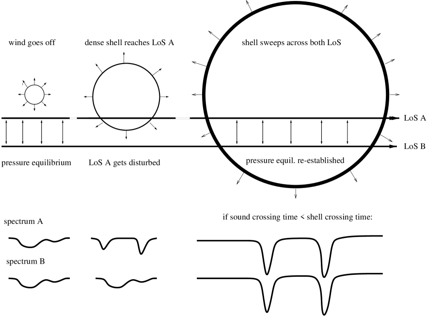
Figure 10: left: A wind bubble expands near two lines of sight ($A$ and $B$). The absorption spectra (bottom of the figure) look identical before the shell hits the first line of sight. Middle: the first line of sight (A) gets disturbed by the passage of the shell. The absorption pattern of $A$ looks very different from that of $B$. Right: after the shell has slowed down sufficiently pressure waves re-establish equilibrium between the lines of sight. The absorption pattern although different from the initial state, looks again the same in both lines of sight.

The upper limit $f_{LoS}\leq 0.23$ on the fraction of disturbed pixels in the Ly$\alpha$ forest can be used in a crude way to estimate the number density and volume filling factor of galactic outflows from their effect on the density field of the IGM, in sofar as such variations appear as differences between the HI column densities (Ly$\alpha$ forest opacities) between two close lines of sight. The principle will be illustrated here for a model of windbubbles expanding into the intergalactic medium (fig. 10).

We assume that dense shells of swept up material occasionally cross the double lines of sight to a lensed background QSO. It can be shown (see Appendix B) that even under unfavorable conditions the shells should have HI column densities high enough to be seen in absorption in a high signal to noise ratio QSO spectrum like the one of Q1422+231 discussed here (N(HI)$>10^{12}$cm^-2). The passage of the shell is very likely to disturb the resemblance between the absorption lines in the two lines of sight (Fig. 10). Ideally, the shell should produce two absorption systems at its two points of intersection with the lines of sight. We assume that there will be measurable differences in the absorption lines between the lines of sight as long as new shell material keeps crossing the lines of sight faster than the differences can be smoothed out by pressure waves travelling at the sound speed. Or in other words, a shell is no longer detectable for when the speed of sound $c$ exceeds the transverse velocity of the shell across the lines of sight:

$$\frac{\dot{R}}{R}b<c,$$ (8)

where $b$ is the impact parameter of the lines of sight relative to the center of the shell, and $R$ and $\dot{R}$ are the radius and expanding velocity of the shell.

To convert the line-of-sight filling factor into a volume filling factor a particular model for the disturbance and its observational signature is needed. For illustrative purposes we adopt the supershell model of MacLow & McCray (1988), i.e., we assume that the disturbances are wind-blown shells escaping from high redshift galaxies. For a given line-of-sight filling factor, the radius $R$, velocity of the shell $\dot{R}$, volume filling factor $f_{v}$, and the space density $n_{gal}$ of galaxies with a wind escaping into the IGM can be written in terms of the mechanical luminosity $L_{38}$ (in units of $10^{38}$ ergs/s), the density of the ambient medium $n_{-5}$ (in units of $10^{-5}$ cm^-3), and the age of the wind bubble $t_{7}$ (in units of $10^{7}$ years). These relations are given in Appendix $B$.

Figures 11 and 12 show the dependence of the upper limits on $n_{gal}$ and $f_{v}$ for winds of various ’strengths’ (i.e., with the ratio $L_{38}/n_{-5}$ as the distinguishing parameter) corresponding to the upper limit $f_{LoS}\leq 0.23$ on the fraction of disturbed pixels in the Ly$\alpha$ forest.

The model is highly oversimplified in that it assumes spherical bubbles with a single age and a single combination of L₃₈ and $n_{gal}$, propagating through a homogeneous medium (and the expansion of the universe is not taken into account), but it contains several features likely to be relevant to more realistic future models (figs. 11 and 12):

1. The number of galaxies with winds originating close to the epoch of observation ($z=3.26$) is essentially unconstrained by an observation of the line of sight filling factor (fig.11). This is because the shell radii are so small that even a large number of galaxies with winds would produce a negligible total absorption cross section.

2. Weak winds (low luminosity and / or large density of ambient medium, i.e., $L_{38}/n_{-5}\leq 1$), because of their limited lifetime, escape detection if they originated early (e.g., before $z_{SF}\sim 4$ for a $L_{38}/n_{-5}\sim 0.1$ shell, or before $z_{SF}\sim 7$ for a $L_{38}/n_{-5}\sim 1$ shell; fig. 11).

3. Strong winds ($L_{38}/n_{-5}>10$) remain detectable even if they started a Hubble time ago (fig. 11), and the upper limit on their numbers becomes stronger with increasing redshift $z_{SF}$.

4. The volume filling factor (fig. 12) is most tightly constrained for recent rather than old winds, independent of strength.

5. Our observation cannot exclude that the universe is filled with ancient, weak wind bubbles because they would no longer be detectable with the present method by redshift $z\sim 3$ (see item 2 above). However, since these weak winds do not reach far out from galaxies and galaxies are not distributed randomly it is very unlikely that such bubbles could fill a substantial fraction of the voids. Strong winds ($L_{38}/n_{-5}>10$) are much better constrained because of their long lifetimes: if winds of strength $L_{38}/n_{-5}\sim 1000$ started as early as $z_{SF}\sim 10$, they could be filling up to about 40% of the volume of the universe by redshift z = 3.26. If such strong winds arose at $z_{sf}\sim 4$ they may fill up to 18% .

4 Conclusions

We have applied various methods to search for and measure density and velocity structure on 100 pc scales in the intergalactic medium at $<z>=3.26$. The smallness of the differences in column density and velocity between the lines of sight confirm and extend the results of Smette et al (1992,1995), and Petry, Impey & Foltz (1998). In the unsaturated regions of the Ly$\alpha$ forest RMS differences between the projected line of sight velocities over 120 pc do not exceed a few hundred meters per second. The RMS total density differences are inferred to be less that 3%, and are basically below the detection limit. Visible differences between the lines of sight do occur occasionally but are localized and seem to be mostly limited to high column density gas. Strong differences are known to occur from studies of the higher column density metal absorption lines (papers I and II), but these differences rarely show up in the Ly$\alpha$ region proper because of saturation. Our results appear broadly consistent with predictions by Theuns, Mo & Schaye (2001) who model the impact of stellar feedback on the appearance of the Ly$\alpha$ forest and find that stellar feedback will mostly affect the higher column density, Lyman Limit absorption systems. The suggestion (Chen et al 2000) that most absorption lines with a rest frame equivalent width $>0.32\AA\$ (corresponding to N(HI)$\sim 6\times 10^{13}$ cm ^-2 for a Doppler parameter $b=28$kms^-1) are related to galactic halos (where we might expect to see hydrodynamic disturbances) is not contradicted by our results because close to 90% of the Ly$\alpha$ forest lines above our chosen column density threshold ($10^{12}$ cm^-2) have lower column densities.

Our results are consistent with unsaturated Ly$\alpha$ systems being mostly featureless at the few percent level on scales smaller by an order of magnitude than state-of-the art cosmological hydro-simulations can currently resolve. Apparently, the finite resolution of the simulations does not lead to a significant underestimate of the clumpiness of the baryon distribution, for densities typical of the unsaturated Ly$\alpha$ forest, i.e., overdensities up to a factor 10-15. However, our observations only provide a snapshot of the properties of the Ly$\alpha$ forest at $z\sim 3.3$ and cannot exclude the existence of earlier non-gravitational processes in the IGM if, by the time of observation, their hydrodynamical traces have been obliterated (see also below).

Notwithstanding doubts about the applicability of the Kolmogorov law to the low density IGM, we have tentatively derived the rate of turbulent energy input into the low density IGM. The turbulent energy in the unsaturated low column density Ly$\alpha$ clouds ($\log N(HI)<14.13$) appears to be lower by 3–4 orders of magnitude than that in the stronger, CIV absorbing clouds dealt with in paper II. Apparently, the CIV gas has been affected more recently (and thus more frequently, given it is unlikely that there is a sharply defined ”epoch” of star formation) by stellar feedback than the general Ly$\alpha$ forest.

The fraction of the spectra that differ by more than 5% in optical depth with respect to the other line of sight, considering all saturated regions as being disturbed, was measured for various column density ranges. The results imply a limit on the relative importance of hydrodynamic disturbances in the presence of the restoring effects of gas pressure. From the upper limit to the line of sight filling factor ($f_{LOS}<23\%$) we find upper limits to the volume filling factor and space density of wind-producing galaxies as a function of the mechanical wind luminosity, the density of the ambient IGM, and the starting redshift of the wind. The presence of short lived, weak winds (low luminosity or high ambient density) is only poorly constrained. The other extreme, long-lived superwinds with $L_{38}/n_{-5}\sim 1000$ arising as early as redshift 10, could fill up to 40% of the volume of the universe by redshift 3.3, but not more than 18% if starting at redshift 4. Currently there is no observational evidence for the existence of $z\sim 10$ superwinds, but closer to the epoch of our observations strong outflows have been seen in high redshift galaxies (Franx et al. 1997; Pettini et al 2001), so there is the possibility that a significant fraction of the volume of the universe may have been stirred by winds; our results appear to show that it is not a dominant one.

5 Appendix A

Our criterion for the optimum choice of the maximum permissible measurement error (chapter 3.2) is as follows: we would like to omit $m$ of the $n$ measurements such that the mean measurement error decreases from $\overline{\sigma_{\rm err}(n)}$ to $\overline{\sigma_{\rm err}(n-m)}$, as long as this reduced error outweighs the decrease in the number of data points available, and continues to lead to a reduction in the error of the determination of the total width of the distribution to be measured, $\sigma_{tot}(n)/\sqrt{n}\rightarrow\sigma_{tot}(n-m)/\sqrt{n-m}$; in other words, we throw away the data points with the largest errors until the uncertainty in the width of the distribution does not improve anymore. Data points should be continued to be omitted as long as

$$E=\left(n-1+S(m)\right)\ \overline{\sigma_{\rm err}^{2}(n)}-\frac{n(n-1)}{n-m}\ \overline{\sigma_{\rm err}^{2}(n-m)}-\sigma_{\rm tot}^{2}(n)\ S(m)>0,$$ (9)

where

$$S(m)=\sum_{k=0}^{m-1}\frac{n(n-1)}{(n-k)(n-k-1)}.$$ (10)

For $m$ = 1, we obtain the simple relation

$$\overline{\sigma_{\rm err}^{2}(n)}-\overline{\sigma_{\rm err}^{2}(n-1)}>\frac{\sigma_{\rm tot}^{2}(n)}{n}$$ (11)

The function $E$ is shown for the distributions of the velocity and column density differences in the bottom panels of figs. 5 and 8. The optimum value of $E$ occurs where $E$ changes from positive to negative values.

6 Appendix B

This appendix addresses two questions: (1) would a superbubble or wind blowing into the IGM at high redshift produce detectable HI absorption, and (2) can we produce limits on the volume filling factor of extragalactic wind bubbles from the fraction of the Ly$\alpha$ forest spectrum disturbed by such events ?

6.1 Detection of HI absorption from dense shells in the IGM

We assume that the dynamics of the wind shell can be described by the superbubble model of Mac Low & McCray (1988). Then the dependence of the radius $R$ on the mechanical luminosity $L=L_{38}\times 10^{38}$ erg s^-1, the time $t=t_{7}\times 10^{7}$ years, and the number density of protons $n=n_{-5}10^{-5}$ cm^-3 in the ambient IGM, is given by

$$R=L_{38}^{1/5}n_{-5}^{-1/5}t_{7}^{3/5}\ 2670\ {\rm pc},$$ (12)

and the expansion velocity is

$$\dot{R}=L_{38}^{1/5}n_{-5}^{-1/5}t_{7}^{-2/5}\ 157{\rm\ kms}^{-1}.$$ (13)

The t͡otal hydrogen column density seen radially outward through the shell is

$$N_{s}(H)=n_{s}\Delta R=\frac{nR}{3}=2.75\times 10^{16}L_{38}^{1/5}n^{4/5}_{-5}t_{7}^{3/5}{\rm cm}^{-2}$$ (14)

The gas density $n_{s}$ in the shell is given by (Weaver et al 1977):

$$n_{s}=n\frac{\dot{R}^{2}+c^{2}}{c_{s}^{2}},$$ (15)

where $c$ is the sound speed in the undisturbed IGM and $c_{s}$ is the sound speed in the shell. The thickness of the shell, $\Delta R$, is

$$\Delta R=\frac{N_{s}}{n_{s}}=\frac{nR}{3n_{s}}=\frac{Rc_{s}^{2}}{3(\dot{R}^{2}+c^{2})}=14.4\frac{L_{38}^{1/5}n^{-1/5}_{-5}t^{3/5}_{7}c_{s,20}^{2}}{L_{38}^{2/5}n^{-2/5}_{-5}t^{-4/5}_{7}+0.0162c_{20}^{2}}{\rm pc}.$$ (16)

The sound speeds are measured in units of 20 kms^-1. The density in the shell is then

$$n_{s}=\frac{6.16\times 10^{-4}L_{38}^{2/5}n^{3/5}_{-5}t^{4/5}_{7}+c_{20}^{2}}{c_{s,20}^{2}}{\rm cm}^{-3}.$$ (17)

It is not clear how exactly the gas is ionized. If it were in photoionization equilibrium with an ionizing UV background radiation field with intensity $J=10^{-21}$ erg cm^-2s^-1Hz^-1sr^-1 the neutral fraction would be approximately (Bergeron & Stasinska 1986):

$$\frac{n(HI)}{n(HII)}=1.67\times 10^{-3}\left(\frac{n_{s}}{10^{-2}{\rm cm}^{-3}}\right).$$ (18)

Thus the HI column density of the shell (from equations 14 and 18) is

$$N_{s}(HI)=\frac{n(HI)}{n(HII)}N_{s}(H)=2.8\times 10^{12}\ n_{-5}^{7/5}L_{38}^{3/5}t_{7}^{7/5}c_{s,20}^{-2}\left[1+0.0162c_{20}^{2}n_{-5}^{2/5}L_{38}^{-2/5}t_{7}^{-4/5}\right]{\rm cm}^{-2},$$ (19)

which is well detectable in absorption in our data. The actual absorption is likely to be stronger (the bubble certainly sweeps up material with higher than average density ($n_{-5}\sim 1$ at $z\sim 3$) in the vicinity of the galaxy from which it originates.

6.2 Expanding shells as revealed by small scale differences in the absorption pattern

A dense shell crossing two adjacent lines of sight separated by a distance $\Delta r$ will produce differences in the column densities as long as the time it takes the shell to traverse the lines of sight is shorter than the sound crossing time $\Delta r/c$ ($=5.8\times 10^{6}$ yr, in the present case). From simple geometric arguments,

$$\frac{\dot{R}}{R}b>c,$$ (20)

where $b$ is the impact parameter of the lines of sight relative to the center of the shell. Thus the shell is detectable for $b>b_{min}=cR/\dot{R}$, and the cross-section $\sigma$ of the shell for producing absorption lines with differences between the lines of sight that have not been ironed out by pressure waves is

$$\sigma = \pi R^{2}\left(1-\frac{c^{2}}{\dot{R}^{2}}\right),\ \ {\rm for}\ \ \dot{R}>c$$ (21)

$$= \ \ \ \ \ \ \ \ \ \ \ 0,\ \ \ \ \ \ \ \ \ \ {\rm for}\ \ \dot{R}\leq c.$$ (22)

The ‘footprint’ of the shell absorption in the Ly$\alpha$ forest spectrum is expected to consist of a pair of absorption lines, and we assume here that each of these is broadened with a velocity width $\Delta v_{fwhm}=46$ kms^-1 (Doppler parameter 28 kms^-1, which is typical for a photoionized Ly$\alpha$ line in the z=3 IGM). Conservatively, we count only the sum of the widths of the two lines as contribution to the disturbance in the Ly$\alpha$ forest spectrum as it is not clear whether the interior of the bubble would produce detectable structure between the lines of sight (it is most likely to produce a clearing in the forest without small scale features).

When expressed in spatial coordinates (at z=3.26) the combined velocity widths of the two lines corresponds to a proper distance $\Delta L=2\Delta v_{fwhm}H(z)^{-1}\approx 206h_{50}^{-1}$kpc. The fraction of the Ly$\alpha$ forest spectrum disturbed by a coeval population of galaxies with space density $n_{gal}$, producing identical, spherically symmetric, expanding wind shells with radii $R$, and expansion velocities $\dot{R}$ would be

$$f_{LoS} = n_{gal}\sigma\Delta L=2n_{gal}\pi R^{2}\left(1-\frac{c^{2}}{\dot{R}^{2}}\right)\frac{\Delta v_{fwhm}}{H},\ \ \ \ {\rm for}\ \ \ \dot{R}>c,$$ (23)

whereas the volume filling factor for the wind bubbles is simply

$$f_{v}=n_{gal}\frac{4\pi}{3}R^{3}=\frac{2}{3}f_{LoS}R\left(1-\frac{c^{2}}{\dot{R}^{2}}\right)^{-1}\frac{H}{\Delta v_{fwhm}}.$$ (24)

Using the Mac Low & McCray superbubble model to get a first crude estimate the quantities $n_{gal}$ and $f_{v}$ can be expressed as functions of the line of sight covering factor $f_{LoS}$, the time $t_{7}$ or redshift $z_{sf}$ when the wind (or star forming episode) started, and the ratio between the mechanical luminosity and the gas density in the IGM, $L_{38}/n_{-5}$. The upper limits on $n_{gal}$ and $f_{v}$ corresponding to the upper limit $f_{LoS}\leq 0.23$ are shown as a function of $z_{sf}$ for various values of the parameter $L_{38}/n_{-5}$ in figures 11 and 12, respectively. The transformation between time and redshift assumes $\Omega_{m}=0.3$ and $H_{0}$ = 50 km s^-1 Mpc^-1.

7 figures

Figure 1: Normalized Ly$\alpha$ forest spectra of the QSO 1422+231 A image in the wavelength region between Ly$\beta$ and Ly$\alpha$ emission. The shaded areas were excluded from the cross-correlation analysis as not belonging to the forest or as being contaminated by known metal absorption lines. The useable Ly$\alpha$ forest region extends over the wavelength range [4747, 5630] Å  or redshift range $z=\left[2.90,3.63\right]$. The maximum beam separation at the short wavelength end of the spectrum is 270 $h_{50}^{-1}$ pc. The slowly varying function at the bottom is the $1-\sigma$ error.

Figure 2: Enlargement of part of the spectrum of Q1422+231. The spectra of the A (solid line) and C (dotted line) images are plotted on top of each other. There is hardly any difference between the spectra, with the exception of a narrow line (which is largely absent in the spectrum of the C image) and some lower column density fluctuations near 5226 Å. This line and the sharp stronger one at 5225 Å can be identified with a SiIV 1394Å interloper from an absorption system at $z=2.74889$. The other absorption features are plausibly attributed to HI Ly$\alpha$. The slowly varying function plotted at the bottom is the $1-\sigma$ error of image A.

Figure 3: cross-correlation function $r(<d>,\Delta v$), for a mean beam separation $<d>$ = 119 $h_{50}^{-1}$ pc, between the Ly$\alpha$ forests in the Q1422+231 A and C image, for the spectral ranges shown in figure 1.

Figure 4: Distribution of the velocity differences $\Delta v$ (= $v_{A}$ – $v_{C}$) for pairs of absorption components. Two components were considered to correspond to each other, when they were nearest neighbors, lay within 30kms^-1 of each other, and had column densities differing by less than 50 %.

Figure 5: Top: RMS difference between the velocities of individually fitted absorption components in the two lines of sight, versus the maximum measurement error permitted for the redshifts in the sample used. Solid dots give the observed width of the $\Delta v$ distribution, open diamonds the width expected on the basis of statistical errors in the velocity determination alone. The dashed shows the width of the observed distribution, convolved with a Gaussian scatter with $\sigma=1.5$ kms^-1. Bottom: function $E$ giving the merit of increasingly getting rid off the data points with the largest error (s.a. fig. 8). The value of $E$ shows the trade-off between omitting measurement points with errors above a certain value, and the consequent reduction in the size of the sample, versus the maximum measurement error accepted in the sample. Positive values of E imply that it is beneficial to continue throwing away points with the largest errors, negative values imply a loss of information. The zero crossing corresponds to the optimum choice. The meaning of $E$ is explained in the text and the Appendix.

Figure 6: Scatter diagram of the logarithmic column densities in the A and C spectrum.

Figure 7: Distribution of the logarithmic column differences $\Delta\log N$ (= $\log N_{A}$ – $\log N_{C}$) for pairs of absorption components. Two components were considered to correspond to each other when they were nearest neighbors, lay within 30kms^-1 of each other, and had logarithmic column densities differing by less than 1.0.

Figure 8: Top: RMS difference between the column densities of individually fitted absorption components in the two lines of sight versus the maximum measurement error permitted for the column densities in the sample used. Solid dots give the observed width of the $\Delta\log N$ distribution, open diamonds the width expected on the basis of statistical errors in the column density determination alone. Bottom: the value of function $E$ shows the trade-off between omitting measurement points with errors above a certain value, and the consequent reduction in the size of the sample, versus the maximum measurement error accepted in the sample. Positive values of E imply that it is beneficial to continue throwing away points with the largest errors, negative values imply a loss of information. The zero crossing corresponds to the optimum choice.

Figure 9: Distribution of differences between the HI optical depth $\Delta\tau=\mid\tau_{A}-\tau_{C}\mid$ for various column density ranges. The fraction of pixels in the column density ranges shown are 100% (solid line), 36.6% (dashed line), 36.4% (dash-dotted line), and 17.4% (dotted line).

Figure 11: Upper limit on the number density of galaxies surrounded by wind bubbles, as a function of the redshift $z_{SF}$ where the wind starts. The diagram is based on a ‘disturbed’ fraction $f_{LoS}\leq 0.23$ of the Ly$\alpha$ forest. The different curves belong to different values of $L_{38}/n_{-5}$. Winds at the low end of the $L_{38}/n_{-5}$ range are less well constrained because they have a shorter lifetime for detection. The mean redshift of observation (3.26) is marked by an arrow.

Figure 12: Upper limit on the volume filling factor for wind blown bubbles. The input parameters are the same as for the previous figure. Strong winds $L_{38}/n_{-5}\sim 100-1000$ can fill a significant fraction of the volume of the universe (up to 40% if they start as early as redshift 10, up to $\sim 18\%$ if they start at z=4), whereas winds with $L_{38}/n_{-5}\leq 1$ are essentially unconstrained if they occur before redshift 7.

References

- (1)
- (2) Aguirre, A., Hernquist, L., Schaye, J., Weinberg, D.H., Katz, N., Gardner, J., 2001, astro-ph/0006345
- (3) Barlow, T.A., Sargent, W.L.W., 1997, AJ, 113, 136
- (4) Bechtold, J., & Yee, H. K. C. 1995, AJ, 110, 1984
- (5) Bergeron J., Stasińska, G., 1986, A&A, 169, 1
- (6) Bryan, G. L., Machacek, M., Anninos, P., Norman, M. L. 1999, ApJ, 514, 13
- (7) Carswell, R.F.,Webb, J.K.,Cooke, A.J., Irwin, M.J., 1992, Institute of Astronomy, Cambridge, http://www.ast.cam.ac.uk/ rfc/vpfit.html
- (8) Carswell, R.F., Lanzetta, K.M., Parnell, H.C., Webb, J.K., 1991, ApJ, 371, 36
- (9) Cen, R., Miralda-Escudé, J., Ostriker, J.P., Rauch, M.. 1994, ApJ, 437, L9
- (10) Cen, R., Bryan, G.L., 2001, ApJ, 546, L81
- (11) Chen, H.-W., Lanzetta, K.M., Fernández-Soto, A., 2000, ApJ, 533, 120
- (12) Couchman, H.M.P., Rees, M.J., 1986, MNRAS, 221, 53
- (13) Croft, R.A., Weinberg, D.H., Katz, N., Hernquist, L.. 1997 ApJ, 488, 532
- (14) Davé, R., Hernquist L., Katz, N., Weinberg, D.H., 1999, ApJ, 511, 521
- (15) Ferrara, A., Pettini, M., Shchekinov, Y., 2000, MNRAS, 319,539
- (16) Franx, M., Illingworth, G.D., Kelson, D.D., van Dokkum, P.G., Tran, K.-V., 1997, ApJ, 486, L75
- (17) Foltz, C.B., Weymann, R.J., Röser, H.J., Chaffee, F.H.. 1984, ApJ, 281, 1
- (18) Hernquist, L., Katz, N., Weinberg, D., Miralda-Escudé, J., 1996, ApJ,457, 51
- (19) Kundic, T., Hogg, D.W., Blandford, R.D., Cohen, J.G., Lubin, L.M., Larkin, J.E., 1997, AJ, 114, 2276
- (20) Lopez, S., Reimers, D., Rauch, M., Sargent, W.L.W., Smette, A., 1999, ApJ, 513, 598
- (21) Mac Low, M.-M., McCray, R., 1988, ApJ324, 776
- (22) Madau, p., Ferrara, A., & Rees, M.J., 2001, ApJ555, 92
- (23) Miralda-Escudé, J., Cen, R., Ostriker J.P., Rauch, M., 1996, ApJ, 471, 582
- (24) Patnaik, A.R., Browne, I.W.A., Walsh, D., Chaffee, F.H., Foltz, C.B., 1992, MNRAS, 259, 1
- (25) Peebles, P.J.E., “Principles of Physical Cosmology”, Princeton University Press; Princeton 1993
- (26) Petitjean, P., Muecket, J.P., , Kates, R.E., 1995, A&A, 295, 9
- (27) Pettini, M., Shapley A., Steidel, C.C., Cuby J.-G., Dickinson, M., Moorwood, A.P.E. , Adelberger, K.L. , Giavalisco, M., 2001, ApJ, 554, 981
- (28) Petry, C.E., Impey, C.D., Foltz, C.B., 1998, ApJ, 494, 60
- (29) Rauch, M., Carswell, R. F., Chaffee, F. H., Foltz, C. B., Webb, J. K., Weymann, R. J., Bechtold, J. Green, R. F., 1992, ApJ, 390, 387
- (30) Rauch, M., Miralda-Escudé, J., Sargent, W.L.W., Barlow, T.A., Weinberg, D.H., Hernquist, L., Katz, N., Cen, R., Ostriker, J.P., 1997, ApJ,489, 7
- (31) Rauch, M., Sargent, W.L.W., Barlow, T.A., 1999, ApJ, 515, 500 (paper I)
- (32) Rauch, M., Sargent, W.L.W., Barlow, T.A., 2001, ApJ, 554, 823 (paper II)
- (33) Sargent, W.L.W, Young, P.J., Boksenberg, A., Tytler, D., 1980, ApJS, 42, 41
- (34) Schaye, J., 2001, astro-ph/0104272, ApJ, in press.
- (35) Smette, A., Surdej, J., Shaver, P.A., Foltz, C.B., Chaffee, F.H., Weymann, R.J., Williams, R.E., Magain, P., 1992, ApJ, 389, 39
- (36) Smette, A., Robertson, J.G., Shaver, P.A., Reimers, D., Wisotzki, L., Koehler, T., 1995, A&AS, 113, 199
- (37) Theuns, T., Leonard, A., Efstathiou, G., Pearce, F.R., Thomas P A., 1998, MNRAS, 301, 478
- (38) Theuns, T., Mo, H.J., Schaye, J., 2001, MNRAS, 321, 450
- (39) Vogt, S.S., et al., 1994, S.P.I.E. 2198, 362
- (40) Wadsley, J., Bond, J.R., Clarke, D., West, M., 1996, Proc. 12th Kingston Conf., Computational Astrophysics, Halifax, 1996 , Astron. Soc. Pac., San Francisco
- (41) Weaver, T.A., McCray, R., Castor, J., Shapiro, P., Moore, R., 1977, ApJ218,377
- (42) Webb, J.K., 1987, PhD Thesis, Cambridge University
- (43) Weinberg, D.H. Miralda-Escudé, J., Hernquist, L., Katz, N.,1997, ApJ, 490, 564
- (44) Weymann, R.J., Foltz, C.B., ApJ, 272, 1
- (45) Young, P.J., Sargent, W.L.W., Boksenberg, A., Oke, J.B. 1981, ApJ, 249, 415
- (46) Zhang, Y., Anninos, P., Norman, M.L., 1995, ApJ, 453, 57
- (47) Zhang, Y., Anninos, P., Norman, M.L., Meiksin, A., 1997, ApJ, 485, 496