Properties of Microlensing Light Curve
Anomalies Induced by Multiple Planets

Abstract

In this paper, we show that the pattern of microlensing light curve anomalies induced by multiple planets are well described by the superposition of those of the single-planet systems where the individual planet-primary binary pairs act as independent lens systems. Since the outer deviation regions around the planetary caustics of the individual planets occur in general at different locations, we find that the pattern of anomalies in these regions are hardly affected by the existence of other planet(s). This implies that even if an event is caused by a multiple planetary system, a simple single-planet lensing model is good enough for the description of most anomalies caused by the source’s passage of the outer deviation regions. Detection of the anomalies resulting from the source trajectory passing both the outer deviation regions caused by more than two planets will provide a new channel of detecting multiple planets.

1 Introduction

Since the first discovery of extra-solar planets around a pulsar PSR 1257+12 from the analysis of planetary perturbations on pulse arrival time by Wolszczan & Frail (1992) and Wolszczan (1994), various groups have detected planets around nearby stars using high precision radial velocity measurements, e.g., around 51 Pegasi (Mayor & Queloz 1995), 47 Ursae Majoris (Butler & Marcy1996), 70 Virginis (Marcy & Butler 1996), and 16 Cygni B (Cochran et al. 1997). Up to now, nearly 60 extra-solar planets are known (http://cfa-www.harvard.edu/planets). From close examination of the velocity residuals to the Keplerian fits to a subsample of 12 planet-bearing stars, Fischer et al. (2001) suggested that nearly 1/2 of the stars may have a second companion. Currently, six systems are identified to have multiple planets: around $\nu$ And (Butler et al. 1999), HD 83443 (Mayor et al. 2001), HD 168443 (Marcy et al. 2001a), G7 876 (Marcy et al. 2001b), HD 82943 and HD 74156 (http://exoplanets.org/mult.shtml).

Although majority of the best candidate extra-solar planets were discovered by the radial velocity technique, they can also be detected by using other techniques. Microlensing is one of the promising techniques, especially to search for planets located at Galactic-scale distances. Planet detections by using microlensing is possible because the event caused by a lens system composed of a planet (or planets) can exhibit noticeable anomalies in the lensing light curve when the source star passes closely to the lens caustics (Mao & Paczyński 1991). The caustic refers to the source position on which the lensing-induced amplification of a point-source event becomes infinity. The lens system with a planet (planets) form several disconnected sets of caustics. Among them, one is located very close to the primary lens, “central caustic”, and the other(s) is (are) located away from the primary lens, “planetary caustic(s)” (Griest & Safizadeh 1998). The planet-induced anomalies last only a few hours to days, and thus it is difficult to detect them from the survey-type lensing experiments (MACHO: Alcock et al. 1993; OGLE: Udalski et al. 1993; EROS: Aubourg et al. 1993; MOA: Abe et al. 1997). However, with sufficiently frequent and accurate monitoring from follow-up observations of ongoing events alerted by the survey teams, one can detect the anomalies and determine the planet parameters of the mass ratio and the instantaneous projected separation between the planet and the primary lens. Currently, several groups are actually carrying out such observations: MPS (Rhie et al. 1999), PLANET (Albrow wt al. 1998), and MOA (Abe et al. 1997).

Along with the observational efforts, planetary microlensing has also been the field of intensive theoretical studies. These include phenomenological studies of the lensing behaviors (Wambsganss 1997; Dominik 1999; Safizadeh et al. 1999), estimation of the detection probability and efficiency (Gould & Loeb 1992; Bolatto & Falco 1994; Bennett & Rhie 1996; Peale 1997, 2001; Gaudi & Sackett 2000), development of the observational strategies for optimal planet detections (Griest & Safizadeh 1998; Han & Kim 2001), and various problems and solutions in determining planet parameters (Gaudi & Gould 1997; Gaudi 1998; Griest & Safizadeh 1998). However, most of these studies were focused on lens systems composed of only a single planet, despite the fact that our solar system is composed of multiple planets. Gaudi, Naber & Sackett (1998) demonstrated that if extra-solar systems are composed of planets having orbital separations comparable to those of Jupiter and Saturn of our solar system, the joint probability of two planets having projected separations within the lensing zone of $\sim 0.6$ – 1.6 of the Einstein ring radius is substantial, invoking the necessity of studies about the lensing properties of multiple planetary systems.

In this paper, we investigate the properties of lensing light curve anomalies induced by multiple planets. Multiple planetary microlensing was first explored by Gaudi et al. (1998). However, since they were interested only in the anomalies occurring near the peaks of the light curves of high amplification events, for which the planet detection efficiencies are high (Griest & Safizadeh 98), they investigated anomaly patterns only in the region around central caustics. In this work, we extend the investigation in wider areas including the outer deviation regions around planetary caustics.

The paper is organized in the following way. We begin with a brief review of the basics of multiple planetary lensing in § 2. In § 3, we present the anomaly patterns of an example lens system and the resulting light curves to illustrate the effect of multiple planets. We discuss about the implications of the new findings in § 4. A brief comment and conclusion are found in § 5.

2 Basics of Multiple Planetary Lensing

A lens system composed of multiple planets is described by the formalism of multiple lensing with very low mass-ratio companions. If a source star is lensed by $N$ point-mass lenses, the locations of the resulting images are obtained by solving the mapping equation (lens equation), which is expressed in complex notations by

$$\zeta=z+\sum_{j}^{N}{m_{j}\over\bar{z}_{j}-\bar{z}},$$ (1)

where $m_{j}$’s represent the mass fractions of the individual lenses such that $\sum_{j}^{N}m_{j}=1$, $z_{j}$’s are the positions of the lenses, $\zeta=\xi+i\eta$ and $z=x+iy$ are the positions of the source and images, and $\bar{z}$ denotes the complex conjugate of $z$ (Witt 1990). We note that all these lengths are normalized by the angular Einstein ring radius, which is related to the total mass, $M$, and the geometry of the lens system by

$$\theta_{\rm E}=\sqrt{4GM\over c^{2}}\left({1\over D_{\rm ol}}-{1\over D_{\rm os}}\right)^{1/2},$$ (2)

where $D_{\rm ol}$ and $D_{\rm os}$ represent the distances to the lens and source from the observer, respectively. The angular separations between the microlensed images are of the order of several milli-arcsecs, which are too small to be resolved. However, the lensing event can be identified by the change of the source star flux. The amplifications of the individual images are given by the inverse of the determinant of the Jacobian of the lens equation evaluated at the image position, i.e.

$$A_{i}=\left(\frac{1}{|{\rm det}\ J|}\right)_{z=z_{i}};\ \ {\rm det}\ J=1-{\partial\zeta\over\partial\bar{z}}{\overline{\partial\zeta}\over\partial\bar{z}}.$$ (3)

Then the total amplification is obtained by the sum of those of the individual images, i.e. $A=\sum_{i}^{N_{I}}A_{i}$, where $N_{I}$ represents the number of images. The caustic corresponds to the source position on which the determinant becomes zero, i.e. $|{\rm det}\ J|=0$. The lens equation describes a mapping from the lens plane onto the source plane. Then, to find image positions $(x,y)$ for a given source position $(\xi,\eta)$, the equation should be inverted.

For a single lens system ($N=1$), the lens equation can be inverted and thus is algebraically solvable, yielding two solutions (and thus the same number of images). The total amplification is expressed in a simple form of

$$A={u^{2}+2\over u\sqrt{u^{2}+4}},$$ (4)

where $u$ is the dimensionless lens-source separation vector normalized by $\theta_{\rm E}$. The separation vector is related to the single lensing parameters by

$$\mbox{\boldmath$u$}\ =\ \left({t-t_{0}\over t_{\rm E}}\right)\ \hat{\mbox{\boldmath$x$}}\ +\ \beta\ \hat{\mbox{\boldmath$y$}}\ ,$$ (5)

where $t_{\rm E}$ represents the time required for the source to transit $\theta_{\rm E}$ (Einstein time scale), $\beta$ is the closest lens-source separation in units of $\theta_{\rm E}$ (impact parameter), and $t_{0}$ is the time at that moment. The unit vectors $\hat{\mbox{\boldmath$x$}}$ and $\hat{\mbox{\boldmath$y$}}$ are parallel with and normal to the direction of the relative lens-source transverse motion.

For a multiple lens system ($N\geq 2$), on the other hand, the lens equation is non-linear and thus cannot be inverted. However, it can be expressed as a polynomial in $z$, and the image positions are obtained by numerically solving the polynomial. For a $N$ point-mass lens system, the lens equation is equivalent to a $(N^{2}+1)$-order polynomial in $z$ and there are a maximum $N^{2}+1$ and a minimum $N+1$ images and the number of images changes by a multiple of two as the source crosses a caustic. Due to the non-linear nature of the lens mapping for a multiple lens system, the lensing behavior of events caused by a multiple lens is not given by a simple superposition of the individual single lens events.

Unless the planet has a separation very close to $\theta_{\rm E}$, a single-planet lens system forms a single central caustic and one or two planetary caustics depending on the projected separation between the primary and the planet. Accordingly, there exist two different types of planet-induced anomalies; one affected by the planetary caustic(s) (“type I anomaly”) and the other affected by the central caustic (“type II anomaly”) (Han & Kim 2001). Compared to the frequency of type I anomalies, type II anomalies occur with a relatively low frequency due to the smaller size of the central caustic compared to that of the planetary caustic(s). However, the efficiency of detecting type II anomalies can be high because intensive monitoring is possible due to the known type of target events (i.e., high amplification events) and the predictable time of anomalies (i.e., near the peak of light curves).

As the number of lenses increases, solving the lens equation becomes very cumbersome. One commonly practiced approach to obtain amplification patterns of these lens systems is the inverse ray-shooting technique (Schneider & Weiss 1986; Kayser, Refsdal & Stabell 1986; Wambsganss 1997). In this method, a large number of light rays are shoot backwards from the observer plane through the lens plane, and then collected (binned) in the source plane. Then the amplification pattern is obtained by the ratio of the surface brightness (i.e., the number of rays per unit area) on the source plane to that on the observer plane and the light curve from a particular source trajectory corresponds to the one-dimensional cut through the constructed amplification pattern. This method has an advantage of enabling one to obtain amplification patterns for an arbitrary number of lenses, but has a disadvantage of requiring large computation time to obtain smooth amplification patterns.

In our analysis of multiple-planet lensing properties, we test lens systems composed of two Jovian-mass planets (and thus $N=3$). This is because if extra-solar systems have planets with orbital separations and mass ratios similar to those of our system, other planets except the two Jovian planets (Jupiter and Saturn) will have mass ratios too small to affect the amplification pattern. In addition, the probability of more than three planets being simultaneously located in the lensing zone will be very small. Besides, this allows us to directly solve the lens equation rather than using the more time-consuming ray-shooting method.

3 Properties of Anomalies

For the investigation of the properties of lensing light curve anomalies induced by multiple planets, we construct maps of amplification excesses. The amplification excess is defined by

$$\epsilon_{\rm tri}={A_{\rm tri}-A_{0}\over A_{0}},$$ (6)

where $A_{\rm tri}$ and $A_{0}$ represent the amplifications with and without planets. With the map, one can obtain an overview of the anomaly patterns not testing all light curves resulting from a large number of source trajectories.

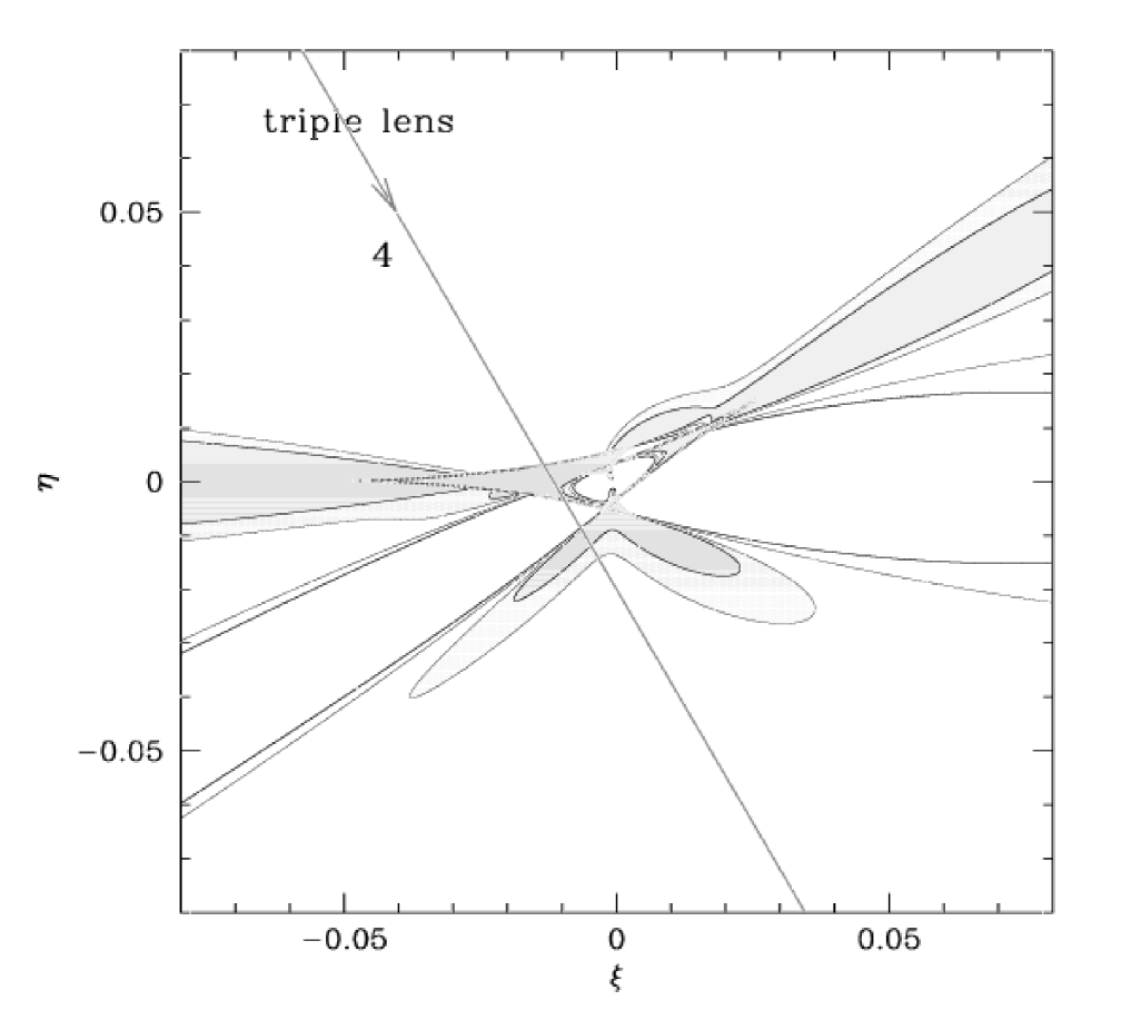
Figure 2: The blowup of the central caustic region of the amplification excess map presented in the upper panel of Fig. 1.

In the upper panel of Figure 1, we present the constructed excess map of an example lens system. The lens system has two planets with mass ratios of $q_{1}=0.003$ and $q_{2}=0.001$, which respectively correspond to those of Jupiter- and Saturn-mass planets around a $\sim 0.3\ M_{\odot}$ star. The individual planets have projected separations (normalized by $\theta_{\rm E}$) of $b_{1}=1.3$ and $b_{2}=0.85$ and the orientation angle between the position vectors from the primary lens to the individual planets is $\phi=150^{\circ}$. In the map, the levels of excesses are represented by contours, which are drawn at the levels of $\epsilon=-10\%$, $-5\%$, 5%, and 10% and the regions of positive excess are distinguished by grey scales. To show the detailed excess patterns in the region around the central caustic, the map of the region is expanded and presented separately in Figure 2.

From the investigation of the map, one may notice an interesting point that the locations of the outer caustics are very similar to those of the planetary caustics of the individual planet-primary binary pairs. To show this similarity more closely, in the lower panel of Fig. 1 we present the excess map constructed by superposing the excesses of the two single-planet lens systems where the individual planet-primary pairs act as independent lens systems (binary superposition), i.e.

$$\epsilon_{\rm bs}=\sum_{i=1}^{2}{A_{{\rm b},i}-A_{0}\over A_{0}},$$ (7)

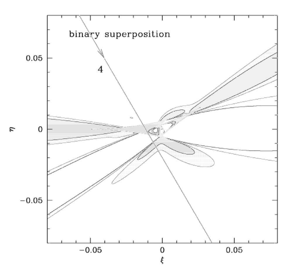
Figure 3: The blowup of the central caustic region of the amplification excess map presented in the lower panel of Fig. 1.

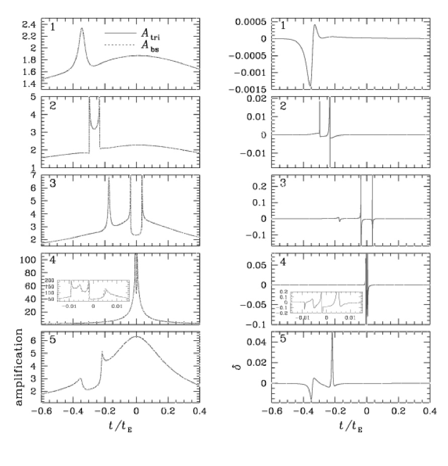
Figure 5: Left panels: The light curves of the events resulting from the source trajectories marked in Fig. 1. The number in each panel corresponds to the trajectory number. Right panels: The curves of the fractional deviations of the amplification obtained by the binary superposition approximation from that of the exact triple lens system.

where $A_{{\rm b},i}$’s represent the binary-lensing amplifications of the individual planet-primary pairs. In Figure 3, we also present the blowup of the central region of the map. From the comparison of the excess patterns in the outer deviation regions, one finds that not only the locations of the outer caustics but also the excess patterns around them are very similar each other. This can be seen also from the comparison of the light curves of events caused by the triple lens system (solid curves in the left panels of Figure 5) to those obtained by the binary superposition (dotted curves in the same panels of the same figure), which are obtained by

$$A_{\rm bs}=A_{0}(1+\epsilon_{\rm bs})=\sum_{i=1}^{2}A_{{\rm b},i}-A_{0}.$$ (8)

From the comparison of the maps in Fig. 2 and 3, one finds that the excess patterns in the region around the central caustic are also similar each other, although the similarities are not as exact as those in the outer deviation region.

To more systematically investigate how accurately the multiple-planet lensing properties can be represented as binary superposition, we compute the fractional deviation of the amplification obtained by the binary superposition from that of the exact triple lens system by

$$\delta={A_{\rm tri}-A_{\rm bs}\over A_{\rm tri}}.$$ (9)

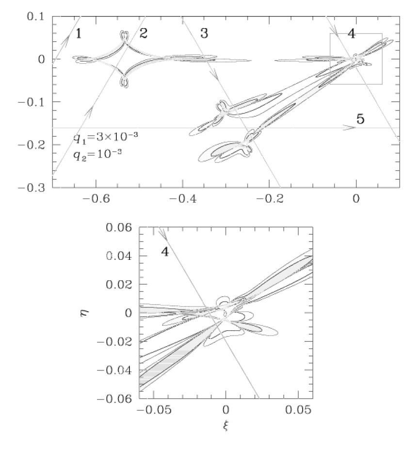
Figure 4: The contour map of the fractional deviation of the amplification obtained by the binary superposition approximation from that of the exact triple lens system. The map is for the same lens system whose excess map is presented in Fig. 1. The contours are drawn at the levels of $\delta=-1\%$, $-0.5\%$, 0.5%, and 1% and the regions of positive $\delta$ is distinguished by grey scales. The lower panel is the blowup of the map in the region around the central caustic.

In Figure 4, we present the contour map of $\delta$ for the same lens system whose excess map is presented in Fig. 1. We note that in the map the contours are drawn at the levels of $\delta=-1\%$, $-0.5\%$, 0.5%, and 1%, which are much smaller than those of the contours in the map of $\epsilon$. In the right panels of Fig. 5, we also present the deviation curves of $\delta$ for the events resulting from the source trajectories marked in Fig. 1. From the map and deviation curves, one finds that the differences occur only in small localized regions very close to the caustics. The spikes in the deviation curves are caused by the shift of the caustics. However, we note that the shift is very small ($\sim 10^{-3}\theta_{\rm E}$), corresponding to the time shift of approximately half an hour for a typical Galactic bulge event with $t_{\rm E}\sim 20$ – 30 days. Considering the photometric precision ($\mathrel{\hbox{\hbox to0.0pt{\hbox{\lower 4.0pt\hbox{$\sim$}}\hss}\hbox{$>$}}}1\%$) and monitoring frequency ($\sim 3$ times/night) of the current microlensing follow-up observations, it will be difficult to notice the caustic shifts. In addition, the modified light curve can be fit by a light curve with very slightly changed lensing parameters. Therefore, the binary superposition will be a good approximation for the description of the example multiple-planet system.

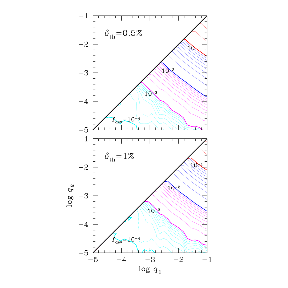
Figure 6: The contours of constant $f_{\rm dev}$, which represents the fraction of the area within the Einstein ring where the binary superposition approximation deviates from the exact lensing amplification more than a threshold value $\delta_{\rm th}$ for the lens systems composed of two planets with mass ratios $q_{1}$ and $q_{2}$. The presented $f_{\rm dev}$ are the values averaged for lens systems with planets having relative orientation angle in the range $0\leq\phi\leq 2\pi$ anf located in the lensing zone, i.e. $0.6\mathrel{\hbox{\hbox to0.0pt{\hbox{\lower 4.0pt\hbox{$\sim$}}\hss}\hbox{$<$}}}b_{i}\mathrel{\hbox{\hbox to0.0pt{\hbox{\lower 4.0pt\hbox{$\sim$}}\hss}\hbox{$<$}}}1.6$. The upper and lower panels are the maps constructed with the threshold deviations of $\delta_{\rm th}=0.5\%$ and $1\%$, respectively.

Then, to what companion mass ratios is the approximation of binary superposition valid for the description of the lensing behavior of multiple-companion systems? To answer this question, we compute the fraction of the area within the Einstein ring where the binary superposition approximation deviates more than a threshold value $\delta_{\rm th}$ for lens systems with various combinations of mass ratios, $f_{\rm dev}(\delta_{\rm th})$. In Figure 6, we present the contours of constant $f_{\rm dev}$ in the parameter space of ${\rm log}\ q_{1}$ and ${\rm log}\ q_{2}$. We note that the presented $f_{\rm dev}$ are the values averaged for lens systems with planets having relative orientation angles in the range $0\leq\phi\leq 2\pi$ and located in the lensing zone, i.e. $0.6\mathrel{\hbox{\hbox to0.0pt{\hbox{\lower 4.0pt\hbox{$\sim$}}\hss}\hbox{$<$}}}b_{i}\mathrel{\hbox{\hbox to0.0pt{\hbox{\lower 4.0pt\hbox{$\sim$}}\hss}\hbox{$<$}}}1.6$. The upper and lower panels represent the maps constructed with the threshold deviations of $\delta_{\rm th}=0.5\%$ and $1\%$, respectively. From the maps, one finds that most lens systems with heavier companion mass ratios of $q_{1}\mathrel{\hbox{\hbox to0.0pt{\hbox{\lower 4.0pt\hbox{$\sim$}}\hss}\hbox{$<$}}}10^{-2}$ have $f_{\rm dev}\leq 1\%$, implying that the lensing behaviors of multiple-planet systems are well approximated by the binary superposition. We note, however, that if $q_{1}\mathrel{\hbox{\hbox to0.0pt{\hbox{\lower 4.0pt\hbox{$\sim$}}\hss}\hbox{$>$}}}0.05$, the fraction becomes considerable [$f_{\rm dev}(\delta_{\rm th}=0.5\%)\mathrel{\hbox{\hbox to0.0pt{\hbox{\lower 4.0pt\hbox{$\sim$}}\hss}\hbox{$>$}}}8\%$ and $f_{\rm dev}(\delta_{\rm th}=1\%)\mathrel{\hbox{\hbox to0.0pt{\hbox{\lower 4.0pt\hbox{$\sim$}}\hss}\hbox{$>$}}}4\%$], implying that the binary superposition approximation will not be appropriate to describe the lensing behavior of systems composed of very heavy planets (with masses $\mathrel{\hbox{\hbox to0.0pt{\hbox{\lower 4.0pt\hbox{$\sim$}}\hss}\hbox{$>$}}}10\ M_{\rm J}$) and brown-dwarf-mass companions.

4 Implications

In the previous section, we show that the patterns of amplification excesses of a lens system composed of multiple planets can be well approximated by the superposition of excesses induced by the planets of the individual planet-primary binary pairs. This finding has the following implications in describing the lensing behaviors of events caused by multiple planetary systems and determining their planet parameters.

The first implication of our finding is that even if an event is caused by a multiple-planet lens system, a simple single-planet lensing model will be good enough for the description of most type I anomalies. This is because the excess pattern in the outer deviation region caused by one of the planets is hardly affected by the other planet component(s). Complication might occur if the outer deviation regions induced by the individual planets occur at a similar place. However, this case is rare since the outer excess region induced by a planet-mass companion occupies a small area.

However, the situation becomes complicated for the type II anomalies. This is because the central deviation regions of the individual planets always occur in the same region regardless of their orientations. As a result, the pattern of anomalies induced by one planet in this region can be significantly affected by the existence of other planet(s), as pointed out by Gaudi et al. (1998). Since one should apply complex multiple-planet lensing models for the description of anomalies occurred in this region, accurate determinations of the planet parameters from the observed light curves will be difficult, as pointed out also by Gaudi et al. (1998).

5 Conclusion

We have investigated the properties of anomalies in lensing light curves induced by multiple planets. From the analysis of the maps of excess amplification and resulting light curves, we find that the excess patterns of a multiple-planet lens system are well described by the superposition of the excesses of the single-planet systems where the individual planet-primary pairs act as independent lens systems. This finding has an important implication that a simple single-planet lensing model is good enough for the description of most type I anomalies even if an event is caused by a lens system composed of multiple planets.

Another interesting point to be mentioned is that detection of the anomalies resulting from the source trajectory passing both the outer regions of deviation induced by more than two planets (e.g., the trajectory designated by a number ‘3’ in Fig. 1) will provide a new channel of detecting multiple planets. The previously suggested method of detecting multiple planets by analyzing anomalies occurred by the source’s passage of the central caustic region (such as the trajectory ‘4’ in Fig. 1) has significant limitations in identifying the existence of multiple planets and determining their parameters due to the degeneracy of the resulting light curves from those of single-planet lensing and the complexity of multiple-planet lensing models. On the other hand, if a multiple-planet lens system is detected through the new channel, one can better determine the planet parameters because the individual anomalies are well approximated by relatively simple single-planet lensing models. We defer a more systematic analysis of this method and estimation of multiple planet detection probabilities for future work.

We thank to B. S. Gaudi for making helpful comments on multiple planetary lensing. This work was supported by a grant (2000-015-DP0449) from the Korea Research Foundation (KRF).

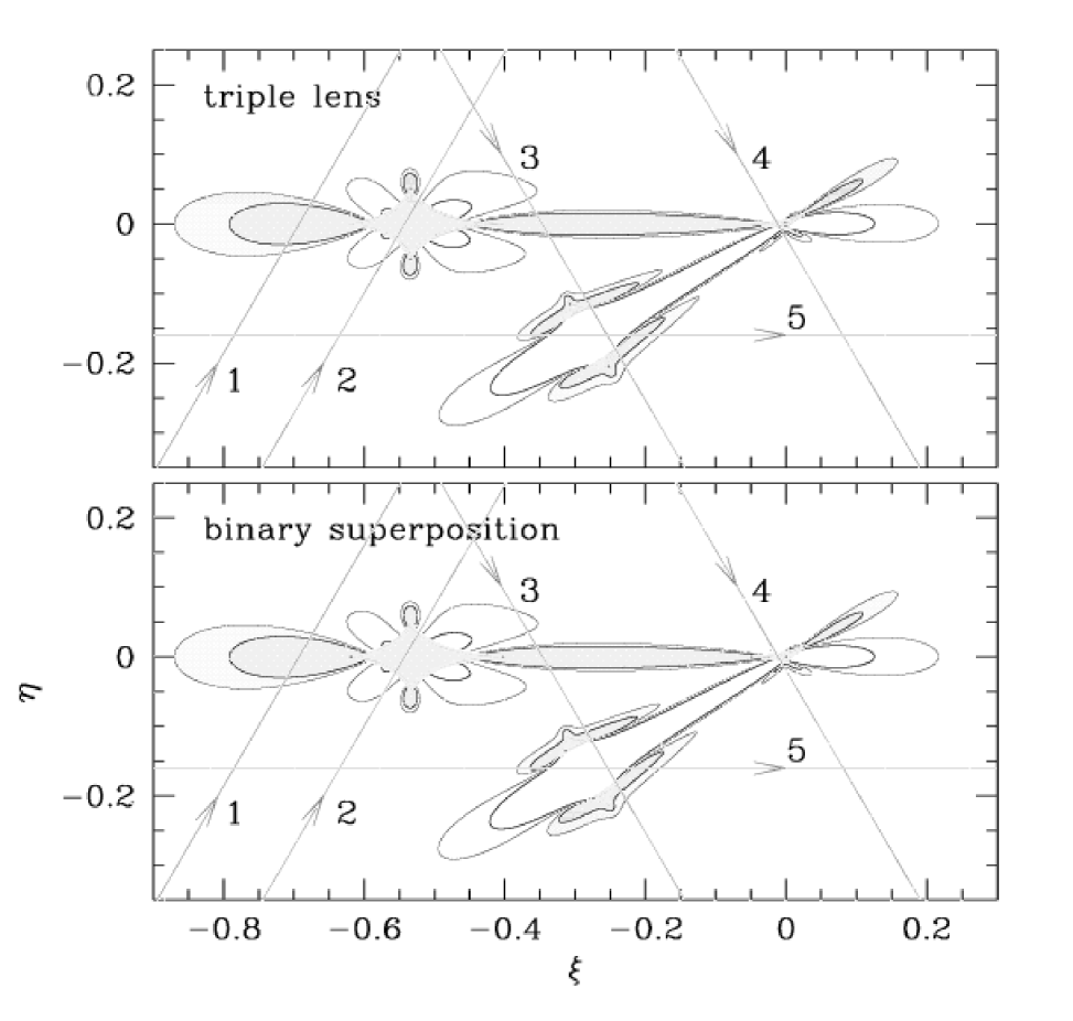
Figure 1: Upper panel: The contour map of amplification excesses of a lens system composed of multiple planets. The lens system has two planets with the ratios of mass to that of the primary of $q_{1}=0.003$ and $q_{2}=0.001$ and the projected separations from the primary of $b_{1}=1.3$ and $b_{2}=0.85$, respectively. The locations are set so that the primary is at the center. The heavier planet is located on the $\xi$ axis on the left side of the primary and the orientation angle between the position vectors to the individual planets (with respect to the primary) is $150^{\circ}$. The contours are drawn at the levels of $\epsilon=-10\%$, $-5\%$, 5% and 10% and the regions of positive excesses are distinguished by grey scales. Lower panel: The excess map constructed by the superposition of excesses of the single-planet lens systems where the individual planet-primary pairs acts as independent lens systems. For both maps, the figures drawn by thick solid line represent the caustics and the straight lines with arrows are the source trajectories of events whose resulting light and excess curves are presented in Fig. 5.

References

- [1] Abe F., et al., 1997, in Variable Stars and Astrophysical Returns of Microlensing Surveys, eds. R. Ferlet, J.-P. Milliard, & B. Raba (Cedex: Editions Frontiers), 75
- [2] Albrow M. D., et al., 1998, ApJ, 503, 325
- [3] Alcock C., et al., 1993, Nature, 365, 621
- [4] Aubourg E., et al., 1993, Nature, 365, 623
- [5] Bennett D., Rhie S. H., 1996, ApJ, 172, 660
- [6] Bolatto A. D., Falco E. E., 1994, ApJ, 436, 112
- [7] Butler R. P., Marcy G. W., 1996, ApJ, 464, L153
- [8] Butler R. P., et al., 1999, ApJ, 526, 916
- [9] Cochran W. D., Hatzes A. P., Butler R. P., Marcy G. W., 1997, ApJ, 483, 457
- [10] Dominik M., 1999, A&A, 341, 943
- [11] Gaudi B. S., 1998, ApJ, 506, 533
- [12] Gaudi B. S., Gould A., 1997, ApJ, 486, 85
- [13] Gaudi B. S., Naber R. M., Sackett P. D., 1998, ApJ, 502, L33
- [14] Gaudi B. S., Sackett P. D., 2000, ApJ, 528, 56
- [15] Gould A., Leob A., 1992, ApJ, 396, 104
- [16] Griest K., Safizadeh N., 1998, ApJ, 500, 37
- [17] Han C., Kim Y.-G., 2001, ApJ, 546, 975
- [18] Kayser R., Refsdal S., Stabell R., 1986, A&A, 166, 36
- [19] Mao S., Paczyński B., 1991, ApJ, 374, L37
- [20] Marcy G. W., Butler R. P., 1996, ApJ, 464, L147
- [21] Marcy G. W., et al., 2001a, ApJ, 555, 418
- [22] Marcy G. W., Butler R, P., Fischer D., Vogt S. S., Lissauer J. J., Livera E. J., 2001b, ApJ, 555, 418
- [23] Mayor M., Naef D., Pepe F., Queloz D., Santos N. C., Udry S., Burnet M., 2001, in ASP Conf. Ser., in press
- [24] Mayor M., Queloz D., 1995, Nature, 378, 355
- [25] Peale S. J., 1997, Icarus, 127, 269
- [26] Peale S. J., 2001, ApJ, 552, 889
- [27] Rhie S. H., Becker A. C., Bennett B. R., Fragile P. C., Johnson B. R., King L. J., Peterson B. A., Quinn J., 1999, ApJ, 522, 1037
- [28] Safizadeh N., Dalal N., Griest K., 1999, ApJ, 522, 512
- [29] Schneider P., Weiss A., 1986, A&A, 164, 237
- [30] Udalski A., Szymański M., Kaluzny J., Kubiak M., Krzemiński W., Mateo M., Preston G. W., Paczyński B., 1993, Acta Astron., 43, 289
- [31] Wambsganss J., 1997, MNRAS, 284, 172
- [32] Witt H. J., 1990, A&A, 263, 311
- [33] Wolszczan A., Frail D. A., 1992, Nature, 355, 145
- [34] Wolszczan A., 1994, Science, 264, 538