A SCUBA Scan-map of the HDF: Measuring the bright end of the sub-mm source counts

Abstract

Using the 850$\,\mu$m SCUBA camera on the JCMT and a scanning technique different from other sub-mm surveys, we have obtained a 125 square arcminute map centered on the Hubble Deep Field. The one-sigma sensitivity to point sources is roughly 3 mJy and thus our map probes the brighter end of the sub-mm source counts. We find 6 sources with a flux greater than about 12 mJy ($>4\sigma$) and, after a careful accounting of incompleteness and flux bias, estimate the integrated density of bright sources $N(>12\,\rm{mJy})=164^{+77}_{-58}\,\rm{degree}^{-2}$ (68 per cent confidence bounds).

1 Introduction

Detections of submillimetre emission from high redshift galaxies highlight the importance of dust in the early history of galaxy formation. Observations using the Submillimetre Common User Bolometer Array (Holland et al. 1999) of small fields down to the confusion limit allow us to estimate the source counts of 850$\,\mu$m sources below 10 mJy. In order to learn more about source counts (and hence to constrain models), the next step is to search for brighter $(>10\,$mJy) objects over somewhat larger $(>100\,$square arcminute) fields.

The population of bright sub-mm sources is not well understood. Current models (Fall, Charlot & Pei 1996; Blain & Longair 1996; Blain 1998; Eales et al. 2000; Rowan-Robinson 2001) for source counts in the sub-mm have been able to account for the observed sources by invoking evolution which follows the $(1+z)^{3}$ form required to account for IRAS galaxies at 60$\,\mu$m, and the powerful radio-galaxies and quasars (Dunlop & Peacock 1990). Euclidean models with no evolution have a slope of roughly $-1.5$ (i.e. $N(>S)\,{\propto}\,S^{-3/2}$), which cannot possibly account for the lack of sources observed. With reasonable evolution (in IRAS-motivated models), the counts steepen sharply at the 10’s of mJy level to roughly $S^{-2.5}$. Given the additional constraint of not overproducing the sub-mm background, the counts of relatively weak sources lead to little variation between the models. However, at the $10$–$30\,$mJy brightness level various evolutionary models (e.g. Guiderdoni et al. 1998) show more parameter dependence. Moreover, given that brighter sources are easier to follow up at other wavelengths, their investigation may help understand the composition of galaxy types and their evolution.

In this paper, we present a new estimate for the number density of sources which are brighter than $12\,$mJy at 850$\,\mu$m. A general discussion of how sources are detected is presented in the next section. To convert the detections into a source count requires a careful study of the flux bias and incompleteness, which are unavoidable due to confusion and non-linear thresholding. Section three describes Monte-Carlo studies used to estimate and correct for these effects and provide a proper number count estimate. Finally we discuss correlations between the SCUBA scan-map and other sub-mm data sets. Comparison with data from other wavelengths is reserved for a longer paper in preparation (Borys et al. 2002).

2 Data collection and analysis

The SCUBA detector is a hexagonal array of bolometers with a field of view of about 2 arcmin. Using a dichroic filter, the radiation is separated into 850 and 450$\,\mu$m bands which are directed toward 37 and 91 element arrays respectively. To sample a large region of the sky, the telescope scans this array along one of three special directions with respect to the array, chosen to ensure that sky is fully sampled. The secondary mirror is chopped at a frequency of $7\,$Hz between a ‘source’ and ‘reference’ position in order to remove fluctuations due to atmospheric emission.

The standard SCUBA scan-map observing strategy uses multiple chop throws in two fixed directions on the sky and an FFT-based deconvolution technique. This may be appropriate for regions where structure appears on all scales, but it is not optimal for finding point sources. The off-beam pattern gets diluted (making it more challenging to isolate faint sources) and the map noise properties are difficult to understand. Our approach is to use a single chop direction and throw, fixed in orientation on the sky. The result is a map that has, for each source, a negative ‘echo’ of equal amplitude in a predictable position. Although the chop was fixed, we scanned in all three directions in order to better distinguish signal from instrumental noise and sky fluctuations.

A total of 61 scans were obtained in 3 separate runs between 1998 and 2000. The shape of the region mapped was a square centred on the HDF and was oriented along lines of constant right ascension and declination. Using SURF (Jenness & Lightfoot 1998) and our own custom software, we are able to isolate and remove large scale features in the maps and estimate the per-pixel noise level by a careful accounting of the per-bolometer noise and the frequency with which each particular pixel is sampled.

2.1 Scan mapping versus Jiggle map mosaics for large surveys

Most extra-galactic sub-mm surveys previously done use a series of jiggle maps to fully sample a large area of the sky. To ensure uniform noise coverage, the number of integrations on a particular jiggle-map field has to be adjusted according to the weather at the time of observation. The noise level across a scan-map composed of individual scans is very uniform, since each pixel is sampled by many different bolometers, whose noise is constant throughout a scan. One advantage of jiggle-mapping is that it is the most used SCUBA observing mode and thus is already well understood. Also, it is known that the observing efficiency, $\epsilon$ (the ratio of time spent collecting data to elapsed real time) for the jiggle-map mode is higher than for scan-mapping, but this is a slightly misleading measure for reasons discussed below.

In section 2.3 we describe how we measure fluxes of point sources by fitting the beam pattern to the map. We denote the reduction in noise by fitting the beam pattern, as opposed to fitting the positive beam alone, by $\xi$. In the case of scan-mapping, where the beam weights are $+1$ and $-1$, we have $\xi_{S}=\sqrt{2}$. The beam weights for jiggle-mapping, $-0.5,+1,-0.5$ lead to $\xi_{J}=\sqrt{3/2}$. We have determined that the observing efficiencies are $\epsilon_{J}\simeq 0.77$ and $\epsilon_{S}\simeq 0.52$ for jiggle and scan-mapping respectively. The nature of the loss of efficiency in both modes is related to the time needed to read out data after each exposure. In the scan-map mode, the sky is sampled 8 times more often than in jiggle-mode, and hence the readout time is longer.

The overall sensitivity to point sources is $\propto\xi\epsilon^{-0.5}$ and, given the numbers above, the jiggle-map and scan-map mode are found to be almost equally sensitive.

The advantage of using scan-mapping over jiggle-maps in studies of the clustering of SCUBA sources is that the latter mode is insensitive to scales larger than the array size. This, coupled with the uniform noise level and nearly equivalent effective sensitivity should make scan-mapping the preferred mode when planning large field surveys.

2.2 Pointing and flux calibration

Reliably determining the pointing of scan-maps containing no bright sources is problematic. To check for evidence of systematic pointing errors in our data, we re-analysed the Barger et al. (2000) HDF/radio fields, which are a set of smaller maps taken within the HDF flanking field. These maps were taken in the well-used jiggle-map mode and were accompanied by several pointing checks and calibration measurements. We compared the maps against our scan-map using a nulling test, finding a shift of $4\,\pm\,3\,$  arcsec  to the west. There is no evidence that this shift is variable across the field. The source of this pointing offset is not entirely understood, though we note the 3 arcsec per sample scan rate of the telescope and that the shift is along the direction of the chop.

The calibration of our map was determined by fitting the beam model to observations of standard calibrators taken during the run. However, many of the scan-map calibrations turned out to be unusable and we had to rely on photometric and jiggle mode calibrations obtained during the runs. Although scan-map flux conversion factors differ from those measured in other modes, it is reasonable to assume that they are related by a constant multiplicative factor. Hence we were able to derive a relative calibration between nights, and by comparing the scan-map against the Barger data, were were able to determine the absolute calibration.

2.3 Source detection

To construct a model beam-shape we artificially added a very bright source into the data and created a map using our analysis pipeline. The positive lobe of the beam was Gaussian, but the negative lobe showed some evidence of smearing. This is not surprising considering that some of the observations were inadvertently taken using an azimuthal chop (4 out of 61 scans), and other observations were affected by the ‘chop-track bug’, which caused the off-beams of some SCUBA datasets to rotate on the sky even though a fixed coordinate frame was requested.

Sources were found by fitting the dual beam pattern, in a least-squares sense, to each pixel in the map. Note that this is equivalent to a convolution of the map with the beam (Eales et al. 2000) except that it also accounts for the pixel by pixel noise.

A total of six sources were found that have a peak to error-of-fit ratio greater than 4. We also rotated the dual-beam pattern by $180^{\circ}$ and used that as a model; only 3 sources were found, two of which are associated with the two brightest sources in the map. Monte-Carlo simulations suggest that the other false positive is not unexpected. As an additional check, the 3 runs were compared by eye to ensure that each source was evident in all subsets of the data. An additional 6 sources were recovered with a S/N between 3.5 and 4.0. Though more likely to be spurious sources, they are still relatively bright and are included to facilitate comparison with data at other wavelengths. A complete list of sources is given in Table 1.

The map shown in Figure 1 is the output from the source fitting algorithm. It must be pointed out that by convolving with the beam, the dual-beam pattern is converted into a triple beam. The positive source now has two negative echos of half the amplitude spaced by the chop throw on either side.

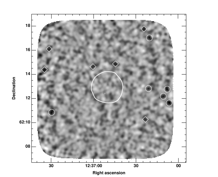
Figure 1: The 850$\,\mu$m HDF scan-map. Black corresponds to positive flux density. The map size is approximately $11.25\times 11.25$ arcminutes. The chop is 40 arcseconds and is roughly east-west. The circles outline the six $>4\sigma$ sources detected in our survey and the diamonds the 6 addition detections above $3.5\sigma$. The region covered by Hughes et al. (1998) is denoted by the white outline near the centre of the map, with their strongest detection, HDF850.1 indicated by the white cross.

Table 1: 850$\,\mu$m detections in the HDF scan-map. The top half of the table lists the $>4\sigma$ sources in order of increasing RA. The last six entries are the weaker detections, again ordered according to RA.

ID	RA(2000)	DEC(2000)	$S_{850}$ (mJy)	S/N
HDFSMM$-$3606+1138	12:36:06.4	62:11:38	$15.4\pm 3.4$	4.5
HDFSMM$-$3608+1246	12:36:07.8	62:12:46	$13.8\pm 3.3$	4.2
HDFSMM$-$3611+1211	12:36:10.6	62:12:11	$12.2\pm 3.0$	4.0
HDFSMM$-$3620+1701	12:36:20.3	62:17:01	$13.2\pm 2.9$	4.6
HDFSMM$-$3621+1250	12:36:21.1	62:12:50	$11.4\pm 2.8$	4.0
HDFSMM$-$3730+1051	12:37:29.7	62:10:51	$14.3\pm 3.2$	4.5
HDFSMM$-$3623+1016	12:36:23.3	62:10:16	$10.3\pm 2.9$	3.5
HDFSMM$-$3624+1746	12:36:24.2	62:17:46	$12.6\pm 3.4$	3.7
HDFSMM$-$3644+1452	12:36:44.5	62:14:52	$11.4\pm 2.9$	3.9
HDFSMM$-$3700+1438	12:37:00.4	62:14:38	$10.1\pm 2.9$	3.5
HDFSMM$-$3732+1606	12:37:31.6	62:16:06	$12.1\pm 3.3$	3.6
HDFSMM$-$3735+1423	12:37:34.9	62:14:23	$13.4\pm 3.8$	3.6

3 Source counts

3.1 Completeness correction

In order to estimate the density of sources brighter than some flux threshold $S^{\prime}$, $N(>S^{\prime})$, we must account for several anticipated statistical effects on our list of detected sources.

1. The threshold for source detection, $S_{T}=m\sigma$ is not uniform across the map due to pixel to pixel noise variation.

2. Due to confusion and detector noise, sources dimmer than $S_{T}$ might be scattered above the detection threshold.

3. Similarly, sources brighter than $S_{T}$ might be missed.

Item (iii) is simply the completeness of our list of sources, and must take into account edge effects and possible source overlaps. For a source density $N(S)$ which falls with increasing flux, item (ii) typically exceeds item (iii), resulting in Eddington bias. Thus measured fluxes tend to be brighter than the true fluxes of the sources.

Using Monte Carlo simulations, these two effects are quantified by measuring $f_{m}(S)$, the fraction of sources at flux $S$ which we would detect above the threshold $S_{T}=m\sigma$. Artificial sources with a range of known fluxes are added to the time series corresponding to random locations (but constrained not to overlap each other) and run through our source detection pipeline.

One can calculate the ratio of the integrated source count to the number of sources we detect,

$$\gamma(S^{\prime})={{{\int_{S^{\prime}}^{\infty}{N(S)dS}}}\over{{\int_{0}^{\infty}f_{m}(S)N(S)dS}}}$$ (1)

where $N(S)dS$ is the number of sources between a flux $S$ and $S+dS$. Note that $f_{m}(S)$ ranges between zero to unity but $\gamma(S^{\prime})$ can be larger than one depending on the form of $N(S)$ and choice of $S^{\prime}$.

The calculation of $\gamma(S^{\prime})$ from the Monte Carlo estimates of $f_{m}(S)$ requires a model of the source counts. We employ the two power-law phenomenological form of Scott and White (1999),

$$N(>S)={N_{0}}{{\left({S}\over{S_{0}}\right)}^{-\alpha}}{{\left(1-{{S}\over{S_{0}}}\right)}^{-\beta}}.$$ (2)

and use $S_{0}=10\,$mJy, $\alpha=0.8$, $\beta=2.5$, and $N_{0}=1.55\times 10^{4}\,{\rm deg}^{-2}$.

Obviously the factor $\gamma$ is influenced by what model is used in the calculation, and other forms of the source spectrum are found in the literature. We find $\gamma$ varies by no more than 10 per cent across a wide range of reasonable parameter values.

This calculation combines all three effects listed above. In the present case, effects (ii) and (iii) balance out almost exactly. We calculate $\gamma(12\,$mJy$)=0.95$, and therefore obtain $N(>12\,$mJy$)=164^{+77}_{-58}\,{\rm deg}^{-2}$ (68 per cent confidence limit) based on the six $4\sigma$ sources found in the 125 square arcminute map. This value is plotted along with estimates from other studies in Figure 2.

3.2 Flux bias correction

Our Monte-Carlo studies confirm the results of Eales et al. (2000) that detected sources tend to be Eddington biased upwards in flux. At the $4\sigma$ level used in this work, our simulations indicate that the boost is 20 per cent in apparent flux; Eales et al. estimate a 40 per cent boost for their $3\sigma$ sources. Note there is no need to use this factor to adjust our estimate of the source counts because it is inherently taken care of in the Monte Carlo simulation and the counts-weighting; We could equivalently quote a somewhat higher source density at 10 mJy.

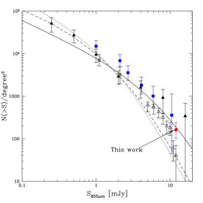
Figure 2: The 850$\,\mu$m source counts. The solid circle shows the result from the current work. Counts derived from cluster studies by Chapman et al. (2001) and Blain et al. (1999) are shown by the solid squares and triangles respectively. The UK 8 mJy survey counts (Scott et al. 2001) are shown as open triangles. Crosses represent the counts from Hughes et al. (1998). Some points are slightly offset along the flux axis for clarity. Overlaid is the two power-law model of Scott & White (solid line), and two predictions based on the models of Rowan-Robinson (2001). The dashed line represents a universe with $\Omega_{M}=1.0$ and $\Omega_{\Lambda}=0.0$ while the dotted line is $\Omega_{M}=0.3$ and $\Omega_{\Lambda}=0.7$.

4 Discussion

We have used other available sub-mm data sets in order to assess the authenticity of our detections. The map of the HDF itself by Hughes et al. (1998) cannot be used for direct comparison because their brightest sources are well below the noise level of this scan-map. Some of sources in the Barger HDF fields previously mentioned are also slightly too faint to be securely detected given the sensitivity of our scan-map, but the brighter ones are found. The average 850$\,\mu$m flux from the seven sub-mm sources in the original Barger catalogue (Barger et al. 2000) is $8.4\pm 0.6\,$mJy in our re-analysis of those data. The average flux from the scan-map at the same seven positions is $8.1\pm 1.1\,$mJy.

Perhaps the most striking feature of the scan-map is the group of three sources on the eastern edge (the first three sources in Table 1). Since the group fits within a single jiggle-map field, we obtained time via the CANSERV program to confirm the existence of these three sources. HDFSMM$-$3606+1138 and HDFSMM$-$3611+1211 differ by no more than $2.5\,$mJy between the scan-map and jiggle-map. HDFSMM$-$3608+1246 is fainter by roughly $5\,$mJy but is still reasonably consistent with the flux derived from the scan-map.

If this trio of sources represent true clustering, then the source count derived here may be biased by cosmic variance. Peacock et al. (2000) have found weak evidence of clustering in the $\sim 2\times 2\,$ arcminute map of Hughes et al. (1998). The UK 8 mJy survey (Scott et al. 2000) which covers over 250 square arcminutes, also shows signs of clustering. However these results are inconclusive, and what is needed is a very large $(\sim\,1$ degree) survey.

We have significantly improved statistics on sub-mm source counts at the $>10\,$mJy level. Because these sources are brighter than typical SCUBA detections, they may be easier to follow up at other wavelengths. Preliminary analysis already indicates good correlation with $\mu$Jy radio sources and hard x-ray sources, but little indication of optical counterparts (as found in other studies).

Based on the re-reduction of the Barger HDF data, we have also found that a careful treatment of the noise map allows us to improve the S/N for point sources by about 15%. Furthermore, we find that scan-mapping is an efficient method for making large maps for cosmological studies. Large-scale spatial instrumental effects do not appear to be a significant limitation for analysis of such maps.

Our careful data-reduction, confirmation in independent jiggle-maps and extensive Monte-Carlo studies lead us to be quite confident in the reality of our six $4\sigma$ sources. We also provide a list of six additional sources between $3.5-4.0\,\sigma$ to aid in comparison with other studies.

References

- [1] Barger A. J., Cowie L. L., Richards E. A., 2000, AJ, 119
- [2] Barger A. J., Cowie L. L., Sanders D. B., 1999, ApJ, 518L
- [3] Blain, A.W., 1998, MNRAS, 295
- [4] Blain A.W., Longair M.S., 1996,MNRAS, 279
- [5] Blain A.W., Smail I., Ivison R., Kneib J., 2000 in A. J. Bunker & W. J. M. van Breughel eds, ASP Conf. Ser. Vol. 193, ASP: San Francisco
- [6] Borys C., Chapman S.C, Halpern M., Scott D. 2002, in preparation.
- [7] Chapman S.C., Scott D., Borys C., Fahlman G., 2002, MNRAS, 330
- [8] Dunlop J.S., Peacock J.A., 1990, MNRAS, 247
- [9] Eales S., Edmunds M.G., 1996, MNRAS, 280
- [10] Eales S., Lilly S., Webb T., Dunn L., Gear W., Clements D., Yun M., 2000, AJ, 120
- [11] Fall S.M., Charlot S., Pei Y.C., 1996, ApJ, 464
- [12] Guiderdoni B., Hivon E.,Bouchet F.R., Maffei B., 1998, MNRAS, 295
- [13] Holland W.S., et al., 1999, MNRAS, 303
- [14] Hughes D.H., et al., 1998, Nature, 394
- [15] Jenness T., Lightfoot J.F., 1998, Starlink User Note 216
- [16] Peacock J., et al., 2000, MNRAS, 318
- [17] Rowan-Robinson M., 2001, ApJ, 549
- [18] Scott D., White M., 1999, A&A, 346
- [19] Scott S., et al., 2001, MNRAS, submitted