THE CLUSTERING PROPERTIES OF LYMAN–BREAK GALAXIES AT REDSHIFT $z\sim 3$

Abstract

We present a new measure of the angular two–point correlation function of Lyman–break galaxies (LBGs) at $z\sim 3$, obtained from the variance of galaxy counts in 2–dimensional cells. By avoiding binning of the angular separations, this method is significantly less affected by shot noise than traditional measures, and allows for a more accurate determination of the correlation function. We used a sample of about 1,000 galaxies with ${\cal R}\leq 25.5$ extracted from the survey by Steidel and collaborators, and found the following results. At scales in the range $30\lower 2.15277pt\hbox{$\;\buildrel<\over{\sim}\;$}\theta\lower 2.15277pt\hbox{$\;\buildrel<\over{\sim}\;$}100$ arcsec, the angular correlation function $w(\theta)$ can be accurately described as a power law with slope $\beta=0.50^{+0.25}_{-0.50}\,(1\,\sigma\,\,{\rm random})\,{}_{-0.10}\,({\rm systematic})$, shallower than the measure presented by Giavalisco et al. However, the spatial correlation length, derived by Limber deprojection, is in very good agreement with the previous measures, confirming the strong spatial clustering of these sources. We discuss in detail the effects of both random and systematic errors, in particular of the so called “integral constraint” bias, to which we set a lower limit using numerical simulations. This suggests that the current samples do not yet provide a “fair representation” of the large–scale distribution of LBGs at $z\sim 3$. An intriguing result of our analysis is that at angular separations smaller than $\theta\lower 2.15277pt\hbox{$\;\buildrel<\over{\sim}\;$}30$ arcsec the correlation function seems to depart from the power–law fitted at larger scales and become smaller. This feature is detected at the $\sim 90$% confidence level and, if real, it can provide information on the number density and spatial distribution of LBGs within their host halos as well as the size and the mass of the halos.

1 INTRODUCTION

A key paradigm of cosmology is that the formation of galaxies, and of the large–scale structure in their spatial distribution, occurred as a result of the action of gravity, which amplified small fluctuations in the primordial mass–density field. Bound structures such as clusters, groups and galaxies formed by gravitational collapse of density perturbations, and star formation took place wherever the local physical conditions have permitted the baryonic gas to condense and cool (White and Rees 1979). Testing this scenario and reconstructing its timing sequence are two major goals of the observations.

A number of studies in the local and moderately distant universe have attempted to use the clustering properties and peculiar velocities of galaxies to test the gravity paradigm (see, for example, Peacock et al. 2001 and references therein). The difficulty with this approach is that, in general, galaxies do not necessarily trace the mass–density field, and their “bias” as generic statistical tracers of the mass distribution is not directly measurable from the data. This bias is also very difficult to model, since it strongly depends on the physics of star formation in galaxies, which is currently poorly understood. While this limitation is probably not severe in the local universe, because the average bias of the present galaxy populations is small (e.g. Taylor et al. 2000; Padmanabhan, Tegmark & Hamilton 2001; Scoccimarro et al. 2001; Feldman et al. 2001), this is not the case at high redshifts, where the bias is very likely significantly larger. Furthermore, peculiar velocities of high redshift galaxies are extremely difficult to measure.

A different approach is to directly compare the observed properties of the galaxy distribution to the predictions of the theory, in which the effects of the bias are explicitly taken into account either by means of specific recipes of star formation coupled with N-body simulations (e.g. Kauffmann et al. 1999; Benson et al. 2000; Wechsler et al. 2001) or with hydrodynamic simulations (Katz, Hernquist & Weinberg 1999; Lewis et al. 2000). In this way, one actually assumes gravity as the main interaction responsible for galaxy and structure formation and tests if this, in combination with the adopted physics of star formation, can satisfactorily reproduce the data. This technique is becoming increasingly popular at high redshifts (e.g. $z>2$), where relatively large and well controlled samples of galaxies are becoming available.

Recently, refinements in color selection criteria have made possible empirical studies of galaxy clustering in the high–redshift universe. Color selection, such as the Lyman–break technique (Steidel et al. 1996, 1998; Madau et al. 1996; Lowenthal et al. 1997) or the photometric redshift one (Budavári et al. 2000; Fernandez–Soto et al. 2001), allows one to efficiently identify classes of galaxies in a preassigned redshift range based on their spectral energy distribution. This has resulted in the compilation of large and well–controlled samples of galaxies at $z>2$ which are suitable for clustering studies (Giavalisco et al. 1998, G98 hereafter; Adelberger et al. 1998, A98 hereafter; Connolly et al. 1999; Arnouts et al. 1999; Giavalisco and Dickinson 2001). Since “Lyman–break galaxies” (LBGs hereafter) essentially consist of actively star–forming galaxies (in comparison, quiescent galaxies at high redshifts are much less efficiently identified with the current instrumentation), a major goal of these studies is to provide empirical information on the physics of star formation and on the effects of the light–to–mass bias in determining the final observed clustering properties of the galaxies.

The most widely used statistics to quantify galaxy clustering is the two–point correlation function, both in its angular – $w(\theta)$ – and spatial –$\xi(r)$– versions. These functions measure the excess probability (with respect to a Poisson point–process) of finding galaxy pairs with a given angular or spatial separation (e.g. Peebles 1980). At high redshifts, where the samples are still too small for more sophisticated studies, the two–point functions are often the only statistics that can be practically used. The important result that came from the high–redshift samples is that at $z\sim 3$ star–forming galaxies are apparently rather strongly clustered, with a (comoving) two–point correlation length that rivals that of the galaxies in the local universe (Steidel et al. 1998; G98; A98; Connolly et al. 1998; Arnouts et al. 1999; Giavalisco & Dickinson 2001). This is interesting, because if the distant galaxies trace the mass in the same way as the local galaxies do, a spatial clustering at $z\sim 3$ almost as strong as at $z=0$ is very difficult to explain simply in terms of gravitational instability. This is true for any reasonable choice of the background cosmology in which the power spectrum of linear density fluctuations is normalized to reproduce the present–day abundance of massive clusters (Eke, Cole & Frenk 1996; Jenkins et al. 1998). If gravity is the interaction responsible for structure formation in the universe, the strong clustering at high redshifts implies that the galaxies at $z\sim 3$ were more biased tracers of the mass distribution than their current counterparts are today, and, in particular, that they resided in regions of the mass–density field that were spatially more clustered than the mass itself on average.

A simple explanation for the strong bias is provided by the theory of biased galaxy formation (White & Rees 1978; Kaiser 1984; Peacock & Heavens 1985; Bardeen et al. 1986) which postulates that galaxies form within virialized dark matter haloes. A general prediction is that the clustering amplitude of the most massive halos at any given epoch is amplified with respect to that of the mass distribution, while very small halos are nearly good tracers of the mass–density field (e.g. Mo & White 1996; Catelan et al. 1997; Porciani et al. 1998). The mechanism explains the observations if the observed galaxies form within relatively massive halos (G98; A98), and also suggests a method to constrain the mass spectrum of the observed galaxies under the assumption of a cosmological model and a spectrum of linear density fluctuations (Giavalisco & Dickinson 2001). In general, the strong clustering of high–redshift galaxies has been regarded as indication of the overall robustness of the theory and as evidence of the reality of galaxy biasing (cf. Pierce et al. 1999; Baugh et al 1999; Governato et al. 1998).

While the detection of a somewhat strong clustering at high redshifts seems to be robust, however, the current samples of LBGs still contain too few objects and cover too small an area of the sky (the largest survey so far covers only $\approx 0.3$ square degrees— cf. Steidel et al. 1999) to accurately measure the correlation function or other clustering statistics. Not only the signal–to–noise of the current measures is of the order of $\sim 3$ at best, but the dispersion of different measures suggests the possibility of systematic errors. Thus, an important goal of the observations is to asses how reliably the clustering properties of LBGs have been determined, and to accurately measure the shape of the correlation function. For example, the correlation length measured by Steidel et al. (1998) and A98 is somewhat larger than the one reported by G98. Giavalisco & Dickinson (2001) find evidence that the correlation length might depend on the UV luminosity of the galaxies, possibly decreasing by as much as a factor of $\approx 3$ when going from ground–based samples with flux limit ${\cal R}\sim 25.5$ to the HDF with ${\cal R}\sim 27$. However, Arnouts et al. (1999) find that the correlation function of galaxies at $z\sim 3$ in the HDF identified with photometric redshifts is only marginally smaller than that of the LBGs of the ground–based sample.

In this paper we present a new, more accurate measure of the two–point angular correlation function, $w(\theta)$, of Lyman–break galaxies at $z\sim 3$ with ${\cal R}\leq 25.5$, and a study of the systematic and random errors involved in the measure. Currently, redshift surveys of LBGs do not yet allow direct, robust measures of their (small–scale) three–dimensional clustering. A valid alternative is to use the available redshift information in the form of a distribution function and deproject the angular (two–dimensional) clustering of the galaxies to derive the spatial one (Peebles 1980). Although projection effects decrease the signal–to–noise ratio in the clustering signal, angular samples generally contain many more galaxies than the redshift ones, and are easier to compile because less subject to the systematics induced by the sampling technique. Moreover, they are insensitive to the effects of redshift–space distortions induced by peculiar velocities. In the case of the LBGs at $z\sim 3$ the method is particularly advantageous, because the redshift distribution is accurately known (e.g. Steidel et al. 1999) and covers a relatively small interval of redshift (see the discussion in G98).

The new measure is based on the method of the counts–in–cells (CIC) applied to the angular positions of the galaxies. We use a sample of 971 LBGs photometrically selected from a ground–based survey in 8 distinct fields. This sample contains $\sim 100$ galaxies more than the compilation of catalogs used by G98; however, the primary motivation to revisit the measure of $w(\theta)$ with the CIC is that this method is significantly less affected by shot noise (and hence more accurate) compared to the estimators used by G98. The CIC technique automatically combines information coming from different scales (in practice, all the separations smaller than a threshold value), as opposed to the traditional estimators, where the distribution of angular separations is binned into relatively small intervals. Since discreteness errors represents the major source of uncertainty at small angular separations, the technique allows one to measure the clustering on small scales with improved accuracy. On the other hand, using the CIC technique one does not really measure the angular correlation function $w(\theta)$, but rather its average over the distribution of separations between all the pairs of points which lie within a cell, $\bar{w}(\Theta)$, as a function of the cell size $\Theta$ (see equations (6) and (B-8) for details). One also has to deal with highly correlated data points when fitting models to the data. These are relatively minor penalties, however, particularly if the correlation function has a simple shape, for example a power-law as it turns out to be the case for LBGs, because then it is straightforward to derive the parameters of $w(\theta)$ from $\bar{w}(\Theta)$ (these functions are directly proportional to each other).

The outline of the paper is as follows. In Section 2 we describe our sample of LBGs. In Section 3 we discuss how we estimated the galaxy correlation function and its uncertainty. In Section 4 we describe our technique for fitting a power-law model to the observed correlation function. In Section 5 we discuss a series of tests to assess the statistical significance of an apparent break in the scale–invariant properties of LBGs at small angular separations. Results from the CIC analysis are cross–checked with a different measure of the correlation function obtained counting galaxy pairs in Section 7. Finally, in Section 8, we summarize our results and discuss their implications for the properties of the hosting halos of LBGs and for models of galaxy formation.

2 THE DATA SET

The high efficiency of the Lyman–break technique at $z\sim 3$ (Steidel, Pettini & Hamilton 1995; Madau et al. 1996; Lowenthal et al. 1997; Dickinson 1998), and the relative ease with which color selection criteria can be quantified and modeled (Steidel et al. 1999), make it particularly advantageous for constructing large and well controlled samples of galaxies that are nicely suited to study galaxy clustering at high redshift (G98; A98; Giavalisco & Dickinson 2001).

Most of the data used in this work have been presented and discussed by G98, and the sample of LBGs considered here largely overlaps with the “PHOT” sample discussed by Giavalisco & Dickinson (2001). The only difference consists in the addition of one more field, dubbed CDFb in Table 1, which was acquired shortly after G98 was written. This field has been obtained with the same instrumental configuration and in similar conditions as the other ones (except the Westphal field —see the discussion in G98), and it reaches the same flux limit. The whole sample thus consists of 8 fields imaged in the custom photometric system $U_{n}G{\cal R}$, which has been designed to enhance the sensitivity to relatively unreddened star–forming galaxies at $z\sim 3$ through the Lyman–break technique (Steidel et al. 1999). As in the previous studies of the clustering properties of LBGs (e.g. see G98; A98; Giavalisco & Dickinson 2001), we have considered as LBG candidates all the objects whose colors satisfy the following relations

$$(U_{n}-G)\geq 1.0+(G-{\cal R})\;;\quad(U_{n}-G)\geq 1.6\;;\quad(G-{\cal R})\leq 1.2\;,$$ (1)

with the additional requirement ${\cal R}\leq 25.5$ imposed to produce a reasonably complete sample. It is important to keep in mind that color criteria designed to select LBGs are, to some extent, arbitrary (see, e.g., Dickinson 1998; Steidel et al. 1999). The definition above is a relatively stringent color cut, and other criteria can certainly be defined that would result in larger samples of high–redshift galaxies. However, as a result of the combined effects of intrinsic scatter in the galaxies’ spectral energy distribution and photometric errors, these would also contain a non negligible number of interlopers at lower redshifts. Since one of the goals of this paper is to measure the spatial correlation length of LBGs by deprojecting the angular correlation function, interlopers represent a source of systematic errors that would bias our estimates, and need to be minimized. With the spectroscopic information available, we have defined the color cuts in equation (1) in order to obtain an optimal balance between the competing requirements of having as large a sample as possible which is also as free of low–redshift interlopers as possible, i.e. maximizing the efficiency (see the discussion in Steidel et al. 1999). In this case, the only significant source of interlopers are galactic stars ($3.4\pm 0.8\%$), and all the galaxies that satisfy equation (1) and that have been confirmed spectroscopically were found to have redshift in the expected range for $U_{n}$-band dropouts, i.e. $2.2\lower 2.15277pt\hbox{$\;\buildrel<\over{\sim}\;$}z\lower 2.15277pt\hbox{$\;\buildrel<\over{\sim}\;$}3.8$. LBG candidates that remain unidentified have spectra with too low a signal–to–noise ratio to allow a secure measure of the redshifts, and in no case was an identified redshift found outside the range expected for LBGs selected using equation (1). It useful to remember, in any case, that conclusions on the clustering properties of the galaxies selected through Equation 1 do not necessarily apply to galaxies at similar redshift that are undetected by these color criteria.

Table 1 details the essential statistics of the individual fields that compound the sample, which includes 971 galaxies that satisfy equation (1), after removing all the objects spectroscopically classified as stars (see Steidel et al. 1999). The average surface density of LBGs with ${\cal R}\leq 25.5$ and its standard deviation are $1.25\pm 0.22$ arcmin^-2, while the mean density over the whole sample is $1.24$ arcmin^-2. Only 469 of these galaxies have spectroscopic redshifts, and we expect some stellar contamination among the $\sim 52$% galaxies of the sample without redshift identification, which we have estimated to be $\sim 1.4\%$.

For the purpose of measuring the clustering properties, we recall that in presence of an unclustered population of spurious objects (with negligible cross-correlation with the LBGs) that contaminate the sample by the fractional amount $f$, the estimated and “true” correlations differ by a factor $1/(1-f)^{2}$ (e.g. Maddox, Efstathiou & Sutherland 1996). This bias affects the amplitude of the two–point correlation function, but does not change its shape. Thus, stellar contamination will systematically bias low our estimates by $\sim 3$%. Note that from the spectroscopic yield of the survey ($\mathrel{\hbox to0.0pt{\lower 3.0pt\hbox{$\mathchar 536\relax$}\hss}\raise 2.0pt\hbox{$\mathchar 318\relax$}}80\%$, Steidel et al. 1999) a strict upper limit to the contamination $1/(1-f)^{2}\sim 1.5$ is obtained if one assumes that all the missed spectroscopic identifications of LBG candidates are interlopers.

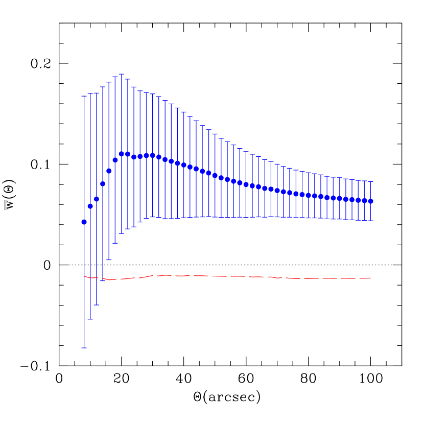
Figure 1: Average correlation function of LBGs (points) estimated computing the factorial moments of the counts, and relative uncertainty (errorbars). The long-dashed line shows the bias of the estimator used to determine $\bar{w}$.

The redshift distribution $N(z)$ of the galaxies selected by means of equation (1) has been very well measured by an extensive spectroscopic program (see Steidel et al. 1999 for a discussion of the observations). We refer to Figure 1 of Giavalisco & Dickinson (2001) for a plot of the function $N(z)$ of the sample discussed here. We will use this function when computing the Limber deprojection of the angular correlation function.

3 MEASURING THE ANGULAR CORRELATION FUNCTION FROM COUNTS–IN–CELLS

We shall now describe how we have measured the correlation function of LBGs from the count statistics. A proper treatment of the shot noise is crucial to reliably extract the information on $w(\theta)$ from low signal–to–noise data like ours. For this reason we have followed two different methods to reconstruct $w(\theta)$ from the counts that adopt very different strategies to account for the shot noise. In one, discussed in §3.1, the contribution of the shot noise is estimated and subtracted. In the other, presented in §3.4, the measure is based on maximum likelihood criteria, adopting a model for the galaxy CPDF. As we shall see, the two methods give consistent results.

3.1 Counts–in–Cells and Factorial Moments

The clustering properties of a distribution of points are completely characterized by the count probability distribution function (CPDF), $P_{N}$, defined as the probability of finding $N$ objects in a randomly placed cell of fixed shape and size. In principle, the CPDF can be estimated from galaxy catalogs (e.g. Szapudi & Colombi 1996) by placing a number $C\gg 1$ of identical cells of given size and shape at random in the sample’s volume, and counting the fraction of cells that contain $N$ objects, i.e.

$$\hat{P}_{N}=\frac{1}{C}\sum_{i=1}^{C}\delta_{N_{i}N}\;,$$ (2)

where $\hat{P}_{N}$ is the estimator of the CPDF, $N_{i}$ is the number of galaxies found in the $i$-th cell, and $\delta_{ij}$ the Kronecker delta symbol .

In practice, even though the CPDF contains all the information about the clustering process, it is often more convenient to look at simpler and more directly interpretable statistics. Commonly used in clustering analysis are the central moments and cumulants of $P_{N}$, which are directly related to the galaxy $N$–point correlation functions (see Appendix A). The factorial moments of order $k$ of the CPDF are defined as

$$F_{k}\equiv\langle(N)_{k}\rangle=\sum_{N}P_{N}(N)_{k}\;,$$ (3)

where $(N)_{k}=N(N-1)\dots(N-k+1)$ is the $k$-th falling factorial of $N$ (e.g. Kendall, Stuart & Ord 1987). Factorial and standard moments are related through the Stirling numbers of the second kind, $S(m,k)$, as follows $\langle N^{m}\rangle=\sum_{k=0}^{m}S(m,k)F_{k}$ (e.g. Szapudi & Szalay 1993). If the point process under analysis (in our case, the galaxy distribution) is obtained by Poisson sampling of an underlying continuous field, the $k$-th factorial moment of the CPDF is equal to the $k$-th standard moment of the continuous field. Then, estimating the factorial moments in a galaxy sample is equivalent to computing the standard moments of the CPDF plus subtracting the shot–noise contribution (see Appendix A).

An unbiased and consistent estimator of $F_{k}$ is

$$\hat{F}_{k}=\frac{1}{C}\sum_{i=1}^{C}\frac{(N_{i})_{k}}{p_{i}^{k}}$$ (4)

(Szapudi & Szalay 1996), where $p_{i}$ is the probability that a galaxy in the cell $i$ has been included in the catalogue (i.e. the product of the selection function and the sampling rate). In the following we will assume that $p_{i}$ has the same (unknown) value for all the cells contained in a given catalogue (i.e. we neglect any small–scale fluctuations due to extinction and inhomogeneities in the CCD frames). We further assume (except where explicitly stated) that fluctuations between the selection functions of different catalogues are negligible (for a detailed discussion about plate to plate variations, see G98).

Szapudi & Colombi (1996) and Szapudi, Colombi & Bernardeau (1999) discussed in detail the problem of estimating the errors of the factorial moments of $P_{N}$. They showed that the proper error generating function (and thus the errors themselves) for a galaxy catalogue which covers a solid angle $S$, and is sampled with $C\gg 1$ cells, $E^{C,S}$, is given by

$$E^{C,S}=\left(1-\frac{1}{C}\right)E^{\infty,S}+E^{C}\;,$$ (5)

where $E^{\infty,S}$ is the error associated with the finiteness of the catalogue (hereafter denoted as “cosmic error”), and $E^{C}$ is the measurement error due to the finite number of cells used for computing $\hat{P}_{N}$. Only $E^{\infty,S}$ quantifies intrinsic properties of the galaxy catalog under analysis, and it represents the minimum uncertainty that can be obtained by extracting the whole information on galaxy clustering from the data. Note that systematic errors introduced during the observation and data reduction are not taken into account by equation (5). To accurately sample the tails of the CPDF it is important to consider the largest possible number of cells. It can be shown that, for large $C$, $E^{C}\propto C^{-1}$ and the corresponding constant of proportionality increases for smaller cells (Szapudi & Colombi 1996). The measurement error then can be made negligible respect to the cosmic variance by considering a sufficiently large number of cells . The ideal case of infinite sampling can actually be achieved in practice using an algorithm developed by Szapudi (1998). Unfortunately, because of the complex geometrical structure of our samples, we could not adopt this method in our analysis.

3.1.1 Estimating the correlation function of LBGs

The connected moments of the galaxy distribution, i.e. the $n$–point correlation functions, can be estimated using non–linear combinations of the factorial moments (Szapudi & Szalay 1993, see also Appendix A). For example, the average of the two–point correlation function over a cell of linear size $\Theta$, which is defined as

$$\bar{w}(\Theta)=\frac{1}{\Sigma^{2}}\int_{\Sigma}d\Omega_{1}\int_{\Sigma}d\Omega_{2}\,w(|\theta_{2}-\theta_{1}|)\;,$$ (6)

where the angles $\theta_{i}$ and $\phi_{i}$ specify a line of sight in the sky, $d\Omega=\sin(\theta)\,d\theta\,d\phi$ is the differential solid angle, $\Sigma=\Sigma(\Theta)$ is the solid angle subtended by the cell, and $w(\theta)$ is the two–point angular correlation function expressed in terms of the angular separation $\theta=|\theta_{2}-\theta_{1}|$, can be estimated using

$$\hat{\bar{w}}=\frac{\hat{F}_{2}}{\hat{F}_{1}^{2}}-1\;.$$ (7)

In practice, we estimated $P_{N},F_{1},F_{2}$ and $\bar{w}$ for our samples in circular cells with 47 (linearly equispaced) radii in the range $8\leq\Theta\leq 100$ arcsec. As we shall discuss below in more detail, the upper limit for the cell size was chosen to minimize edge effects, while the lower bound was set because the shot-noise increases rapidly with decreasing $\Theta$. For each cell size, we have determined the number of cells necessary to estimate the CPDF and its moments as follows. We initially set $C=10^{6}$ and estimated $\bar{w}$ several times times using different seeds for the pseudo–random number generator to determine the actual positions of the cells. If the variance between the estimates was found larger than the $1\%$ of the corresponding average value, we increased $C$ by a factor of ten and repeated the procedure. We found the following optimal values: $C=10^{8}$ for $11<\Theta<25$ arcsec, $C=10^{7}$ for $25\leq\Theta<55$ arcsec, and $C=10^{6}$ for $\Theta\geq 55$ arcsec. All the sets of counts–in–cells used to determine the variance have then been combined together to estimate the CPDF. In order to minimize CPU-time, we used $C=10^{8}$ also for $\Theta=8$ and $10$ arcsec even though this corresponds to $\sim 3\%$ measurement error. As we shall see in the next section, the uncertainty in the estimate of $\bar{w}$ due to cosmic variance decreases from $\sim 200$% to $\sim 30$% when the cell radius is increased from 8 to 100 arcsec. Thus, a random error of $\sim 1$–3% is, for practical purposes, negligible compared to the cosmic error. Note that using $C=10^{6}$ at $\Theta=8$ arcsec would have caused a measurement error of order of $40\%$.

Figure 1 shows the average correlation function measured with the CIC technique described above together with the error bars, computed as described in the following section. Note that $\hat{\bar{w}}$ decreases monotonically for $\Theta>30$ arcsec, it is approximately constant in the range $20$ and $30$ arcsec, and it decreases again for $\Theta\lower 2.15277pt\hbox{$\;\buildrel<\over{\sim}\;$}20$ arcsec. As we will discuss in Section 4, for $\Theta\lower 2.15277pt\hbox{$\;\buildrel>\over{\sim}\;$}40$ arcsec $\bar{w}(\Theta)$ is very well modeled by power-law with slope $\sim-0.5$. At smaller scales this model does not adequately describe the data. It is important to determine if this apparent break in the scale–invariant clustering properties of the LBGs is real, derives from systematic errors in our analyses, e.g. from incorrect shot-noise subtraction, or is simply due to statistical fluctuations. This will be the subject of §5.

3.2 Error estimation

To leading order in $\Sigma/S$ ($\Sigma$ and $S$ are, respectively, the solid angles subtended by a cell and the survey) and assuming Poisson sampling (hereafter PS, see Appendix A), the cosmic error in the estimate of the factorial moments (and, thus, of the correlation functions of any order) can be broken into three components (see, e.g., Szapudi & Colombi 1996):

• the discreteness error. Sampling a continuous field with a finite number of points always causes loss of information. In particular, recovering the statistical properties of the underlying field from the analysis of the corresponding point process becomes increasingly uncertain when the average density of sampling points is decreased. For counts–in–cells studies, this error increases towards small scales and considering higher order statistics;

• the edge effect error. To minimize boundary effects, only cells which are completely included in the galaxy sample must be considered. As a result, the central part of each field is oversampled with respect to the regions lying near the boundaries. This introduces a bias in $\hat{P}_{N}$ whose magnitude increases with the cell size. In our case, for $\Theta=100$ arcsec (circular cells) the effective surface of the LBGs samples (i.e. the area containing the centers of the cells) only covers the $\sim 45\%$ of the whole sample. Moreover, the fraction of cells included in each individual field is proportional to its effective surface. Thus, as a result, the weight of the Westphal sample in the estimate of $\hat{P}_{N}$ increases with the cell size. For instance, considering circular cells with radii in the range from 8 to 100 arcsec, the fraction of cells lying in the Westphal frame moves from 0.30 to 0.39;

• the finiteness error. Estimating the clustering properties of a point–process from a finite sample is, in general, affected by random statistical uncertainties, which arise from the lack of information on the fluctuations of the density-field on scales larger than the sample size. This finite–volume error is proportional to the average of the two–point correlation function over the whole sample. The ensemble average of the finiteness error is known as the integral constraint bias (e.g. Peebles 1980).

Szapudi & Colombi (1996) computed the leading order contributions to the errors for $\hat{F}_{1}$ and $\hat{F}_{2}$ assuming PS and hierarchical scaling of the moments. Their results depend on the field geometry, galaxy surface density and the correlation functions of third and fourth order. Unfortunately, in the case of the LBGs, no information on the $n$–point functions with $n>2$ is available (a discussion on the higher order cumulants of the CPDF will be presented in a future work). Furthermore, our sample consists of a number of sub–samples with different sizes. For these reasons, we did not derive the errors analytically, and we estimated the variance and bias of our statistics with a non-parametric method, namely using the bootstrap resampling technique (Efron 1979). In particular, to account for galaxy correlations, we adopted a variant of the (unmatched) blockwise–bootstrap method developed for the analysis of time–series (Künsch 1989). First, we divided the whole sample into 10 sub–samples covering nearly the same area on the sky. In particular, each of the seven $9\times 9$ arcmin² fields of Table 1 has been considered as a sub–sample, while the Westphal field has been separately divided into 3 additional sub–samples. We then built $B=100$ “bootstrap samples” each of them composed by 10 sub–samples randomly drawn from the set described above. The sub–samples were not matched together to build larger fields, since this procedure would have changed the galaxy clustering properties. Estimates of the CPDF, $\hat{P}_{N}^{\rm(b)}$, the first two factorial moments, $\hat{F}_{1}^{\rm(b)}$ and $\hat{F}_{2}^{\rm(b)}$, and for the average correlation function, $\hat{\bar{w}}^{\rm(b)}$, have been derived for each artificial sample with the same procedure adopted for the real data, and we have estimated the variance of the statistics $\hat{\cal S}$ as

$$\hat{\sigma^{2}}_{\hat{{\cal S}}}=\displaystyle{\frac{1}{B-1}}\displaystyle{\sum_{b=1}^{B}}\left[\hat{{\cal S}}^{\rm(b)}-\langle{\hat{{\cal S}}^{\rm(b)}}\rangle\right]^{2}\;,$$ (8)

where $\langle\hat{\cal S}^{\rm(b)}\rangle=\sum_{b=1}^{B}\hat{\cal S}^{\rm(b)}/B$. The absence of a large, Westphal–like sub–sample is the only difference between the original samples and the bootstrap galaxy samples. This implies that edge and finite–volume effects will be slightly more important in the bootstrap samples, particularly for large cells, and we expect that the error bars will be slightly overestimated.

Our estimates of $(\hat{\sigma^{2}}_{\hat{{\cal S}}})^{1/2}$ are shown in Figure 1. Note that the signal–to–noise ratio for the average correlation function equals 1 at $\Theta\simeq 15$ arcsec. We compared our results with the predictions of Szapudi & Colombi (1996) evaluated for a single $9\times 9$ arcmin² subcatalogue, adopting reasonable values for the hierarchical amplitudes of the higher order correlations of the LBGs – i.e., assuming that they are of the same order of magnitude of the values for local galaxies measured from the APM survey (Gaztañaga 1994; Szapudi et al. 1995). Bootstrap and analytical variances show the same trend with the cell size; however, as expected, the bootstrap estimates of $\sigma_{\hat{F_{1}}}$ and $\sigma_{\hat{F_{2}}}$ are approximately a factor of $\sim 3$ smaller than their analytical counterparts, since we combined together the data from all the samples, while we could compute the analytical one only from one. Furthermore, Colombi et al. (2000) have shown that analytical methods overestimate error amplitudes by a factor of $\sim 2$ at small scales, although this result has been obtained for three-dimensional data, in a regime with negligible discreteness errors.

The mean value of a non–linear combination of two stochastic variables with non–vanishing variance generally differs from the same combination of their mean values. Therefore, the statistics $\hat{\bar{w}}$, which is obtained from the ratio of the unbiased statistics $\hat{F}_{1}$ and $\hat{F}_{2}$, is a biased estimator of $\bar{w}$, namely $\langle\hat{\bar{w}}\rangle\neq\bar{w}$. To quantify the bias let us introduce the parameter $b_{\hat{\bar{w}}}=\langle\hat{\bar{w}}\rangle-\bar{w}$. Analytical estimates for the expectation value of $b_{\hat{\bar{w}}}$ are available to leading order in $\Sigma/S$ (Bernstein 1994; Hui & Gaztañaga 1999; Szapudi, Colombi & Bernardeau 1999), and show that the bias results from a combination of discreteness, edge, and finite volume effects. Thus, we expect $b_{\hat{\bar{w}}}$ to decrease if the variances of $\hat{F}_{1}$ and $\hat{F}_{2}$ become smaller, i.e. by considering larger and larger galaxy samples. Note that $b_{\hat{\bar{w}}}$ includes also the so–called “integral constraint” bias (e.g. Peebles 1980) which derives from using the observed galaxy number density as an estimator of the mean density of the parent population. For relatively small samples, this is, more probably, an overestimate because of the existence of positive correlations between the galaxy positions at small separations. In other words, identifying the sample mean density with the population value corresponds to assuming that the average correlation function over the surveyed region vanishes, i.e. positive correlations at small scales are balanced by a spurious lack of power at large separations. In our case, the galaxy sample is actually the combination of several fields obtained in different areas of the sky, and since all the sub–samples are covered with cells of the same size and shape, we automatically used the average density over the whole sample to normalize the correlation function. This reduces the integral constraint bias. If $S_{i}$ is the surface of the $i$-th sub–sample and $\Theta_{i}$ its linear size, the integral constraint bias of $\hat{\bar{w}}$ is proportional to $[\sum_{i}S_{i}^{2}\bar{w}(\Theta_{i})]/(\sum_{i}S_{i})^{2}$. This result neglects the contribution by discreteness effects as in Bernstein (1994) and Hui & Gaztañaga (1999; see Szapudi, Colombi & Bernardeau (1999) for the general case). As expected, the combination of statistically independent data leads to an increased accuracy.

We estimated the bias of $\hat{\bar{w}}$ using the blockwise bootstrap method, namely

$$\hat{b}_{\hat{\bar{w}}}=\langle{\hat{\bar{w}}^{\rm(b)}}\rangle-\hat{\bar{w}}\;,$$ (9)

where we computed $\hat{\bar{w}}$ from the whole sample with no resampling. Results are shown in Figure 1 together with the measure of $\bar{w}(\Theta)$. As expected (Szapudi, Colombi & Bernardeau 1999; Hui & Gaztañaga 1999), on average, the biased estimator $\hat{\bar{w}}$ tends to underestimate the actual clustering amplitude at all scales. For small angular separations, the bias is negligible with respect to the scatter due to cosmic variance. At larger scales, $\hat{b}_{\hat{\bar{w}}}$ and $(\hat{\sigma^{2}}_{\hat{\bar{w}}})^{1/2}$ become comparable because of increasingly larger edge–effects.

3.3 Analysis Of the Individual Catalogues

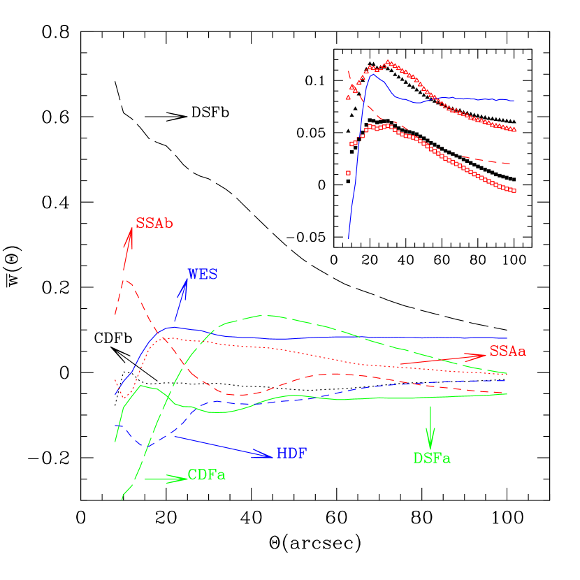
Figure 2: Average correlation function of LBGs estimated computing the factorial moments of the counts in 8 different field. In the inset, the average of the correlations shown in the main panel (squares) is compared with the results obtained in Section 3.1 (triangles). Open and filled symbols refer to quantities computed excluding or including the Westphal field, respectively. The dashed line shows the standard deviation between the functions shown in the main panel. The continuous line marks the correlation function in the Westphal field.

In Section 3.1, we computed the angular two-point correlation function of LBGs combining together all our data. The results have been obtained throwing cells, at random, over all the fields simultaneously (hereafter, method 1). In principle, this can generate systematic errors due to field-to-field variations of the actual limiting magnitude, and photometric zero-points. Many physical effects as variable atmospheric conditions, galactic obscuration, and intergalactic extinction can be responsible for such inhomogeneities. Hence, to minimize spurious inter-field fluctuations of the density of objects, we also measured $\hat{\bar{w}}$ for each single field, and averaged the results over the catalogues (hereafter, method 2). The drawback of this method is that it is affected by a strong integral constraint bias, which, following the discussion in §3.2, we estimate to be at least $5$ times larger than for the technique used in Section 3.1 (this is obtained assuming negligible field-to-field variations). Our results are presented in Figure 2. As expected, fluctuations between the functions $\hat{\bar{w}}$ of different fields are huge, often larger than the correlations themselves. This happens for two reasons, the presence of intrinsic fluctuations of the clustering amplitude among the different samples, and large fractional fluctuations in the mean density reflecting either that inter-field variations are large, or that the correlation function on the scale of the fields is not negligible. It is practically impossible to distinguish between the contributions due to the different effects. As discussed in Section 3.2 of G98, however, we do not expect field–to–field variations due to “observational accidents” (i.e. due to varying observing conditions) to introduce a large spurious contribution to the observed clustering signal. The discrepancy between the results derived with the two methods should be mostly ascribed to the integral constraint bias, which is proportional to the average correlation function, $\bar{w}$, evaluated on the typical scale of a single field. An estimate of the correlation function on the scale of $\sim 9$ arcmin can be obtained from the variance of galaxy counts in our $9\times 9$ arcmin² fields. However, since we only have 7 “cells”, the measurement error is large. We find $\hat{\bar{w}}=0.026\pm 0.013$. Note that this is probably an underestimate since we treated the different fields as independent. The discrepancy between the correlation function obtained averaging over the fields (represented by squares in the inset of Figure 2) and the results obtained with method 1 (shown with triangles) is $\sim 0.05$, independently of the scale. This is an estimate of the difference between the integral constraint bias of method 2 and the (probably small) systematic error arising from inter-field variations (for method 1). Note that the resulting bias is of the same order of magnitude of the signal. Estimators similar to method 2 have been used by G98, who assumed that systematic errors due to the integral constraint were negligible. Their estimates for the correlation function of LBGs might then be biased low.

3.4 The Maximum Likelihood Analysis

In this section we will remeasure the function $\bar{w}(\Theta)$ with a maximum likelihood analysis, avoiding any direct shot-noise subtraction. In this case, discreteness effects are taken into account adopting a model for the galaxy CPDF. The motivation for such a study is to determine how different treatments of shot-noise affect the measure of the galaxy correlation function. In particular, it is fundamental to check if the somewhat surprising behaviour of $\bar{w}(\Theta)$ at $\Theta<30$ arcsec shown in Figure 1 is caused by discreteness effects (see also §5 for a specific discussion). For this reason, the results of the maximum likelihood analysis will be cross–checked with those obtained in the previous sections by measuring the factorial moments of the CPDF.

The method of maximum likelihood provides a robust solution to the problem of estimation. Its key idea is that the best estimate of a parameter is that giving the highest chances that the observed set of measurements will be obtained. Knowledge of the probability of obtaining a set of observations from a population is then required. In order to apply maximum likelihood analyses to the case of galaxy counts–in–cells, it is therefore necessary to make a strong “a priori” assumption for the shape of the population CPDF (and, depending on the method adopted, for the nature of the fluctuations of its estimates, obtained from finite samples, around the expectation value). Inappropriate models or assumptions will obviously result in biased estimates for the average correlation function.

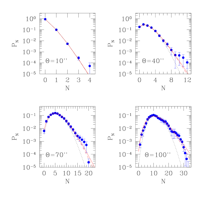
Figure 5: Best-fitting models to the measured CPDF obtained using the Kolmogorov–Smirnov test. Points denote the best estimates of the CPDF from the data. Bootstrap errorbars are also drawn. The dotted lines show the Poisson distributions with the same average counts of the observed CPDF. The dashed and continuous lines represent, respectively, the best-fitting negative binomial and lognormal models.

To the best of our knowledge, no theoretically justified model for the CPDF of the projected distribution of galaxies is available. For the maximum likelihood analysis, we then adopt two phenomenological models for the CPDF, the first is an extension of the negative binomial distribution and the second is the result of Poisson sampling a lognormal distribution. In both cases, the agreement with the data (see Figure 5) seems good enough to justify their use as first analytical approximations to the observed distribution.

3.4.1 The Negative Binomial Distribution

The negative binomial (or modified Bose–Einstein) distribution has been used to describe the PDF of discrete counts in a number of different fields ranging from various branches of physics, to biostatistics and econometrics. In a series of independent binary events (success or failure), having the same chances of success, the negative binomial distribution accounts for the probability of the number of trials necessary for the occurrence of a given number of successes. Among the most widely used discrete distributions, it represents the classical example for overdispersion (with respect to the Poisson distribution), since it is characterized by $\langle(N-\bar{N})^{2}\rangle>\bar{N}$, where $\langle N\rangle=\bar{N}$. In cosmology, it has been originally adopted to describe the distribution of galaxy counts in a Zwicky cluster (Carruthers & Minh 1983) and then it has been extensively used in three-dimensional counts-in-cells analyses (e.g. Ueda & Yokoyama 1996 and references therein).

The dispersion of negative binomial distribution is characterized by an integer parameter. We adopt here a modified version in which the measure of the correlation is real valued:

$$P^{\rm nb}_{N}=\frac{\bar{N}^{N}}{N!}(1+\bar{w}\bar{N})^{-N-1/\bar{w}}\prod_{i=1}^{N-1}(1+i\bar{w})\;.$$ (10)

Elizalde & Gaztañaga (1992) showed how this distribution is obtained by modifying the Poisson process to account for binary interactions between the points. In practice, $\bar{w}$ corresponds to a attraction/repulsion parameter, and $P_{N}^{\rm nb}$ is obtained populating the cells sequentially (adding one object at a time), and assuming that the probability that a point belongs to a cell is proportional to the number of points which are already occupying this cell.

3.4.2 The Discretized Lognormal Distribution

The PDF of the mass density contrast is expected to be lognormal to a good approximation (e.g. Coles & Jones 1991; Kofman et al. 1994; Bernardeau & Kofman 1995). Because of this, it has often been assumed that also the three-dimensional galaxy counts are lognormally distributed. Here, we use a Poisson-sampled lognormal distribution to model the two-dimensional galaxy counts

$$P_{\rm ln}=\frac{1}{N!}\int_{-\infty}^{\infty}\frac{dz}{[2\pi\ln(1+\bar{w})]^{1/2}}\exp{\left\{\displaystyle{Nz-\exp(z)-\frac{\{z-\ln[\bar{N}/(1+\bar{w})^{1/2}]\}^{2}}{2\ln(1+\bar{w})}}\right\}}\;,$$

This choice is not inspired by any theoretical motivation, and it is mainly dictated by simplicity.

Note that both $P^{\rm ln}_{N}$ and $P^{\rm nb}_{N}$ are hierarchical (i.e. the correlation functions of order $j$ $\bar{w}_{j}=K_{j}\bar{w}^{j-1}$ with $K_{j}$ a constant) and reduce to the Poisson distribution when $\bar{w}\to 0$.

3.4.3 Likelihood for the CPDF

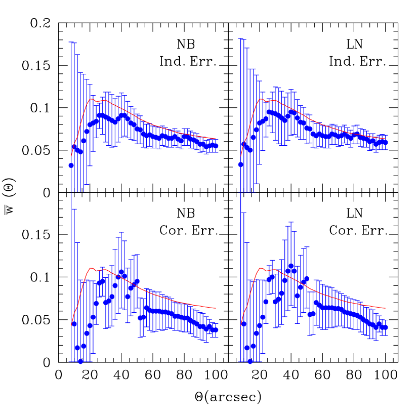
Figure 3: Average correlation function of LBGs estimated performing a maximum likelihood analysis of the CPDF (points with errorbars). The continuous line shows the best estimate of $\bar{w}$ in Figure 1. Left and right panels have been obtained assuming that the CPDF approximates a negative binomial and a Poisson sampled lognormal distribution, respectively. For each $\Theta$, to reduce the effects of statistical fluctuations, only the values of $N$ that have been measured in at least 1000 different cells have been considered for the maximum likelihood analysis. In the top panels, errors in the CPDF at different values of $N$ are assumed to be statistically independent. In the bottom panels, principal component analysis is used to deal with correlated errors. The number of principal components included in the analysis has been fixed by requiring that they accounted for the 95% of the total variance.

It has been recently proposed to directly use the CPDF for maximum likelihood analyses (Kim & Strauss 1998). For this purpose, it is necessary to know how the estimates $\hat{P}_{N}$, derived from finite samples, are distributed around the corresponding population values $P_{N}$. For three-dimensional counts–in–cells, this problem has been addressed by Szapudi et al. (2000) using very large $N$-body simulations. For our two–dimensional problem, we studied the nature of these fluctuations ($\Delta P_{N}=\hat{P}_{N}-P_{N}$) using bootstrap resampling. As Szapudi et al. (2000), we also find that the distribution of each $\Delta P_{N}$ is non-Gaussian (and, for a given cell’s size, its skewness depends on $N$). Only in the tails of the CPDF, where $P_{N}$ is very low, errors nearly follow a Poisson distribution (cf. Kim & Strauss 1998). Moreover, fluctuations at different values of $N$ are correlated (the covariance matrix of the $\Delta P_{N}$ must be singular because of the normalization constraint of the CPDF, $\sum_{N=1}^{\infty}P_{N}=1$). Writing a likelihood function which takes into account all these constraints is extremely challenging. Luckily, useful approximations that also provide some insight into the characteristics of the unknown distribution functions are available. In order to allow for correlations, we use a principal component analysis (see §4.1 for a brief definition) of the $\Delta P_{N}$ resulting from the bootstrap analysis, and, to work with with a relatively simple likelihood function, we assume Gaussian errors. This seems to be a reasonable approximation, since the distribution of the eigenvectors of the covariance matrix (i.e. the principal components) indeed closely resemble a Gaussian function. Note that, when only a subset of principal components is considered, the assumption of gaussianity does not imply assuming that all the $\Delta P_{N}$ are normal variables, which in general will not be true. Subsequently, we write a Gaussian likelihood function (taking into account a finite number of principal components of $\Delta P_{N}$) and we look for its maximum value by varying $\bar{w}$. To deal with a one-dimensional minimization procedure, a value for $\bar{N}$ must be specified a priori. We considered two possibilities: the average density for the whole sample and $\hat{F}_{1}$ corresponding to the cell size under analysis. Similar results are obtained in the two cases. The use of $\hat{F}_{1}$, however, results in a smoother correlation function. The results, shown in Figure 3, are in good agreement with our previous findings, confirming the presence of a small-scale break in the estimated angular correlation function. The most striking feature is that the new estimate of the correlation are biased low respect to those derived from the factorial moments of the CPDF. These results change only slightly when Gaussian and independent errors for $\Delta P_{N}$ are assumed.

The Gaussian assumption could be easily released deciding not to keep track of cross-correlations between different values of $N$ (e.g. Kim & Strauss 1998). In this case, we could directly adopt the probability distribution deriving from the bootstrap analysis: ${\cal L}(\bar{w})\propto\Pi_{N}P_{\rm boot}(\Delta P_{N})$. However, an accurate determination of the tails of $P_{\rm boot}$ would require extremely large amounts of CPU time, and the results would be in any case questionable. We did not follow this approach.

3.4.4 Likelihood for Cell Counts

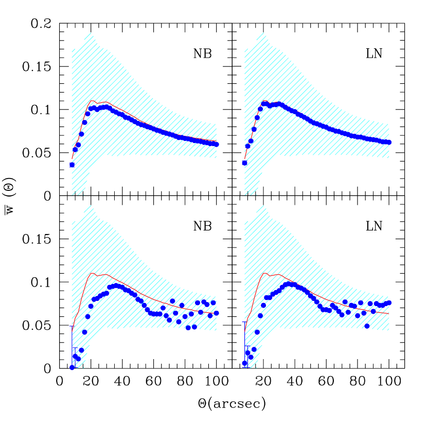
Figure 4: Top: Average correlation function of LBGs estimated performing a maximum likelihood analysis of the counts–in–cells (filled points). Errorbars (which are smaller than the symbols used to mark the best fitting values) denote only measurement errors, and should be combined with cosmic errors to obtain the full uncertainties. The continuous line and the shaded region show the best estimate for $\bar{w}$ in Figure 1 and its total uncertainty. Left and right panels have been obtained assuming a negative binomial and a Poisson sampled lognormal CPDF, respectively. Bottom: Average correlation function for LBGs estimated performing a Kolmogorov–Smirnov test on the CPDF. The notation is as in the top panel.

A widely diffused technique for the estimation of $\hat{\bar{w}}$ consists in applying maximum likelihood methods directly to cell counts (e.g. Efstathiou et al. 1990; A98). In this case, the likelihood is simply the joint probability distribution of the observed counts. This quantity reduces to the product of one–point probabilities whenever the cells are statistically independent (strictly speaking, this never happens when the cells are extracted from the same catalogue because of the density modes with wavelength larger than the separation between the centers of the cells). Independence is obviously violated in our case of overlapping cells. However, if we assume to have a fair sample of galaxies, one can invoke ergodicity to associate the counts in different cells with different realizations of the density field. In other words, if the size of the survey under analysis is much larger than any correlation length, statistically independent cells will dominate the spatial average (Szapudi & Colombi 1996). In practice, this means that, if one analyzes a fair sample, results obtained maximizing the likelihood function ${\cal L}(\bar{w})\propto\Pi_{i=1}^{C}P_{N_{i}}$ should be correct even though the assumption of statistical independence of the cells in the observed sample is not. Biased estimates for $\bar{w}$ are obtained if the sample under analysis is not representative of the whole universe. Note the similarity between this method and the analysis of factorial moments: in both cases massive oversampling of a finite portion of a process is used to extract information about expectation values over the ensemble. We used this method to estimate $\bar{w}$. Our results are shown in the top panels of Figure 4. The almost perfect agreement with the correlation obtained computing the factorial moments is striking and reinforces our confidence on the overall robustness of our measure. Note that the error bars, determined looking for the interval that corresponds to a decrement of $\log{\cal L}$ by $1/2$ from its maximum value, quantify only measurement errors and do not include cosmic errors.

3.4.5 Kolmogorov-Smirnov Test

Since none of the maximum likelihood analyses discussed in the previous section is rigorous from the conceptual point of view, in this section we apply the Kolmogorov–Smirnov test to compare the observed cumulative distribution function ${\cal C}_{N}=\sum_{j=0}^{N}P_{N}$ to the negative binomial and lognormal models (cf. Ueda & Yokoyama 1996). The value for $\bar{w}$ which corresponds to the highest significance level is taken as the estimate for the population value. Results are shown in the bottom panels of Figure 4. An apparent small–scale break in the correlation function is observed in this case as well.

Note the discrepancy at large scales between the different estimates of $\bar{w}$, whose nature can be understood by looking at Figure 5: neither of the two models for $P_{N}$ adopted in the maximum likelihood analysis is able to accurately describe the measured galaxy counts for large cell’s sizes. This is because the observed $P_{N}$ sharply drops when $N$ reaches a maximum value, while the models predict a smooth decrement of the count probability. An excess of counts with respect to the model is also detected for values of $N$ slightly smaller than the cutoff. We tested that the observed drop is not caused by the finite number of cells used in our analysis. After increasing by a factor of 10 the total number of cells used in the CIC analysis, we verified that the shape of the CPDF remained unchanged.

4 FITTING THE DATA WITH A POWER–LAW MODEL

It is customary to fit the observed correlation function (or its average, as in our case) with a power–law model, $\bar{w}(\Theta)=A\Theta^{-\beta}$. In this section, we describe how we have combined a least squares method with a principal component analysis of the bootstrap errors to derive the best fitting power–law to the results obtained with the CIC analysis (Figure 1). Since both the techniques that we have used to estimate $\bar{w}(\Theta)$ consistently return a correlation function that departs from a power–law on small scales, we have separately considered a fit over large angular scales only as well as a “global” fit. We have then compared the results obtained in these two cases to quantify the statistical significance of the apparent “break”.

4.1 Principal Component Analysis of the Errors

Cosmic errors for the average correlation function evaluated at different angular separations are strongly correlated. After defining $\Delta_{i}=[\hat{\bar{w}}(\Theta_{i})-\langle\hat{\bar{w}}(\Theta_{i})\rangle]/\sigma_{\hat{\bar{w}}(\Theta_{i})}$ (with $\sigma_{\hat{\bar{w}}}$ the standard deviation of the estimator $\hat{\bar{w}}$), we estimate the covariance matrix $C_{ij}=\langle\Delta_{i}\Delta_{j}\rangle$ using the bootstrap method described in Section 3.2, $\hat{C}_{ij}=[\sum_{b=1}^{B}\Delta_{i}^{\rm(b)}\Delta_{j}^{\rm(b)}]/(B-1)$, with $\Delta_{i}^{\rm(b)}=[\hat{\bar{w}}^{\rm(b)}(\Theta_{i})-\langle\hat{\bar{w}}^{\rm(b)}(\Theta_{i})\rangle]/[\hat{\sigma^{2}}_{\hat{\bar{w}}(\Theta_{i})}]^{1/2}$. It turns out that $\hat{C}_{ij}$ is a quasi-singular matrix, since all its components differ from one by less than a few percent.

The principal components of a $N$-dimensional random vector are linear combinations of its $N$ components, that are statistically orthonormal and form a complete basis. Since any covariance matrix is symmetric, the principal components of the correlation errors coincide with the eigenvectors of $\hat{C}_{ij}$. In fact, the eigenvectors of the covariance matrix are linear combinations of the errors, $E_{i}^{(n)}=\alpha_{ij}\,\Delta_{j}$, whose variances are given by the corresponding eigenvalues, $\lambda_{n}$. Different eigenvectors are statistically orthogonal (i.e. $\langle E^{(n)}\,E^{(m)}\rangle=\lambda_{n}\,\delta_{nm}$), and uncorrelated (since $\langle\Delta_{i}\rangle=0$) . By ranking the eigenvectors in the order of descending eigenvalues (starting from the largest), one can create an ordered orthogonal basis with the first eigenvector having the direction of the largest variance of the data.

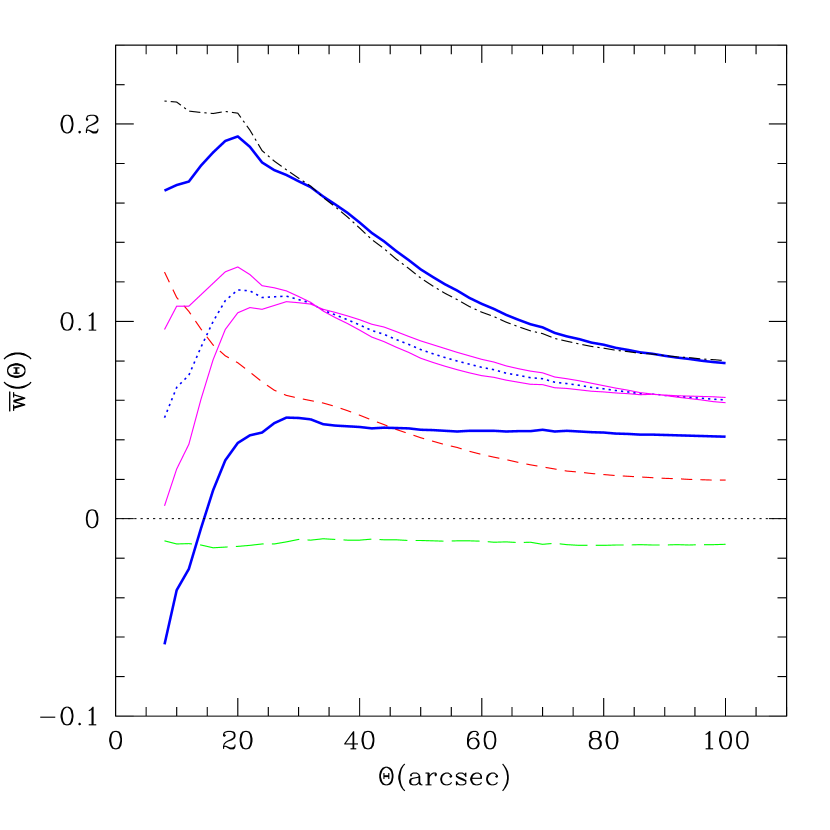
Figure 6: Principal components of the correlation errors. The best estimate of the average correlation function is marked by the points. The short dashed line denotes the size of the 1$\sigma$ errorbars in Figure 1. Note that the signal-to-noise ratio equals 1 for $\Theta\simeq 15$ arcsec. The long-dashed line shows the bias of the estimator used to determine $\bar{w}$. The continuous lines are obtained displacing the data points proportionally to the first two principal components of the errors. The top and bottom heavy lines correspond to a pure first principal component error with amplitude $\pm 1/\sqrt{\lambda_{1}}$ (which, in a standard least squares analysis corresponds to $\chi^{2}=1$). The intermediate light lines correspond to a pure second principal component error with amplitude $\pm 1/\sqrt{\lambda_{2}}$ (again corresponding to $\chi^{2}=1$). The dash–dotted line is obtained combining first and second principal components each with amplitude $1/\sqrt{\lambda_{i}}$ (i.e. has $\chi^{2}=2$). Note how the shape of the correlation function is poorly constrained by the data, especially on small scales.

We reduced the covariance matrix $\hat{C}_{ij}$ to its diagonal form using the LAPACK routines for singular value decomposition (Anderson et al. 1999). The first principal component (which is the minimum distance fit to a line in the $\Delta$-space) comes out to be $E^{(1)}\simeq(1,\dots,1)/\sqrt{N_{\rm fit}}$ and $\lambda_{1}\simeq N_{\rm fit}$, with $N_{\rm fit}$ the dimension of the $\Delta$-space (as discussed in the next section we consider data sets with different dimensionality). Note that the $E^{(1)}$ accounts for a large fraction (typically, $\mathrel{\hbox to0.0pt{\lower 3.0pt\hbox{$\mathchar 536\relax$}\hss}\raise 2.0pt\hbox{$\mathchar 318\relax$}}96\%$) of the variance of the bootstrap data. This means that the $N_{\rm fit}$ residuals lie along a line with a relatively small scatter. In other words, for a given realization, cosmic errors tend to have the same sign and the same amplitude when expressed in units of $(\hat{\sigma^{2}}_{\hat{\bar{w}}})^{1/2}$. As a consequence of this, the normalization of the average correlation function and its shape are poorly constrained by the data. This is another manifestation of large uncertainty in the mean surface density of LBGs due both to statistical fluctuations and to the fact that galaxies are spatially correlated on the sample scale. Figure 6 shows how $\hat{\bar{w}}$ is affected by the most typical error configurations: a monotonically decreasing correlation on all-scales, as well as a flat curve for $\Theta>30$ arcsec are compatible with the data.

4.2 Least Squares Fitting

In order to fit a power-law function to the data for the average correlation function, we use a least squares method. In practice, we minimize

$$\chi^{2}=\sum_{i}\frac{\epsilon_{i}^{2}}{\lambda_{i}}\;,$$ (11)

where $\epsilon_{i}$ represents the projection of the vector of the residuals,

$$\Delta^{\rm(fit)}=\left\{\frac{A\Theta_{1}^{-\beta}-\hat{\bar{w}}(\Theta_{1})}{\left[\hat{\sigma^{2}}_{\hat{\bar{w}}(\Theta_{1})}\right]^{1/2}},\dots,\frac{A\Theta_{N}^{-\beta}-\hat{\bar{w}}(\Theta_{N})}{\left[\hat{\sigma^{2}}_{\hat{\bar{w}}(\Theta_{N})}\right]^{1/2}}\right\}$$ (12)

along the $i$-th principal component, namely $\Delta^{\rm(fit)}=\sum_{i}\epsilon_{i}E^{(i)}$. Note that, for $N_{\rm fit}=47$, the eigenvalues of $\hat{C}_{ij}$ span over 8 orders of magnitude, and can be as small as $\sim 10^{-7}$ (we verified this by solving for the eigenvalues of the correlation matrix using the LAPACK routines for singular value decomposition). Thus, the value of $\chi^{2}$ will be typically dominated by the contribution coming from the principal components with the smallest variances. However, fitting functions which deviate from the data only along the highest-order principal components should not be necessarily rejected. In fact, $\hat{C}_{ij}$ is only an estimate of the “true” covariance matrix and contains an intrinsic uncertainty. These errors propagate in the computation of eigenvalues and eigenvectors combining also with numerical round-off errors, especially for quasi–singular matrices. It is therefore reasonable to consider only the most-stable linear combinations of the data (i.e. the eigenvectors of $\hat{C}_{ij}$ corresponding to the largest eigenvalues) in the fitting procedure. The problem is to determine how many principal components must be discarded. This issue is obviously related to the size of the uncertainties in the correlation matrix. We can identify two sources of errors: the finite number of bootstrap resamplings we used to compute the ensemble average, and the finite number of cells we used to compute the factorial moments. We know that the latter is going to produce $\sim 1\%$ relative errors in $\hat{\bar{w}}$, which cause $C_{ij}$ to be systematically underestimated by $\sim 10^{-4}[(\bar{w}_{i}/\sigma_{\hat{w}_{i}})^{2}+(\bar{w}_{j}/\sigma_{\hat{w}_{j}})^{2}]$. The off-diagonal elements of the matrix $C_{ij}-\hat{C}_{ij}$ should then lie in the range $10^{-3}-10^{-4}$ (all the diagonal elements are, by definition, equal to 1).

What about the other source of error? An unbiased estimate of the random uncertainty due to the finite number of resamplings for $k_{2}=\langle[\hat{\bar{w}}^{\rm(b)}(\Theta_{i})-\bar{w}^{\rm(b)}(\Theta_{i})]^{2}\rangle$ is given by $(2B\hat{k}_{2}+(B-1)\hat{k}_{4})/[B(B+1)]$, where $\hat{k}_{2}$ is computed as in equation (8), $\hat{k}_{4}=B^{2}[(B+1)m_{4}-3(B-1)m_{2}^{2}]/[(B-1)(B-2)(B-3)]$ is the estimated $4^{\rm th}$ order cumulant of $\hat{\bar{w}}^{\rm(b)}(\Theta_{i})-\bar{w}^{\rm(b)}(\Theta_{i})$ with $m_{i}$ the sample $i$-th central moment (Kenney & Keeping 1951, 1962). The relative error on $k_{2}$ decreases with $\Theta$, ranging from $5\times 10^{-3}$ to $2\times 10^{-5}$ with typical values of $\sim 10^{-4}$. Assuming that errors on the $i-j$ covariances are of the same order of magnitude, one gets that uncertainties in $\hat{C}_{ij}$ are a few times $\Delta\hat{k}_{2}/\hat{k}_{2}$, i.e. of order $10^{-2}-10^{-5}$. As a final check, we split our bootstrap realizations into two halves and compared the corresponding correlation matrices: the maximum discrepancy was found to be of order $10^{-2}$, while the typical one was $\sim 10^{-3}$. It is important to remember that, if the errors in the components of a matrix are uncorrelated and of order $\epsilon$, then the errors in the eigenvalues are also of order $\epsilon$. Most importantly, errors significantly change the direction of the eigenvectors corresponding to $\lambda_{i}<\epsilon$. This would suggest to include in the $\chi^{2}$ calculation only the first few eigenvectors. However, the situation changes when the errors in the different components of a matrix are strongly correlated. In this case, the direction of the eigenvectors is barely affected by the errors. Therefore, there is no strict rule to select the number of principal components, but it could be risky to consider eigenvectors corresponding to noisy eigenvalues. Even though some simple (but totally empiric) criteria for the selection of the components are commonly used in factor analysis, we prefer here to explore a number of different cases, using the fraction of variance which has been accounted for as a guiding parameter.

Both bootstrap resampling and the analysis of mock galaxy catalogues (see §5.1) show that, analyzing a finite galaxy sample, it is more probable to underestimate $\bar{w}$ than to overestimate it. This becomes more and more evident with increasing $\Theta$. In absence of a robust maximum likelihood method (the probability density function of $\Delta_{i}$, and the correlation matrix $C_{ij}$ are not known a priori), a simple way to account for the positive skewness of the distribution of the residuals is realized by using our least–squares method after correcting the data for the bias of the correlation estimator. We will use this technique in the following section.

4.3 Results

Because of the shape of $\bar{w}(\Theta)$, which does not resemble a single power law over the whole range of angular separations that we have studied, we have determined the best–fitting power–law functions to the results obtained with the CIC analysis (Figure 1) in two different intervals, $8\leq\Theta\leq 100$ arcsec, and $40<\Theta\leq 100$ arcsec. We performed a number of $\chi^{2}$ minimizations, increasing the number of principal components of the residuals, and, for comparison, we also computed the best–fitting function assuming independent errors. The results, both with and without correction for the bias of our estimator, are listed in Table 2 and Table 3. The range of values of the parameters $A$ and $\beta$ that corresponds to $\Delta\chi^{2}<1$ (i.e., for Gaussian residuals, the $68\%$ confidence levels) is also given in the tables. The low values of $\chi^{2}_{\rm min}$ per degree of freedom ($\chi^{2}_{\rm min}/{\rm d.o.f.}$) obtained considering only the first few principal components suggest that they cannot efficiently discriminate among different power-law models. On the other hand, including too many principal components, one gets very high values of $\chi^{2}_{\rm min}/{\rm d.o.f.}$ and, as expected, the quality of fit worsen dramatically (not shown in the tables). In general, when a power-law gives a fairly good description of the data, the preferred values of $A$ and $\beta$ keep stable with increasing the number of principal components until a threshold is reached. Adding more components significantly changes the best–fitting values $A_{\rm best}$ and $\beta_{\rm best}$.

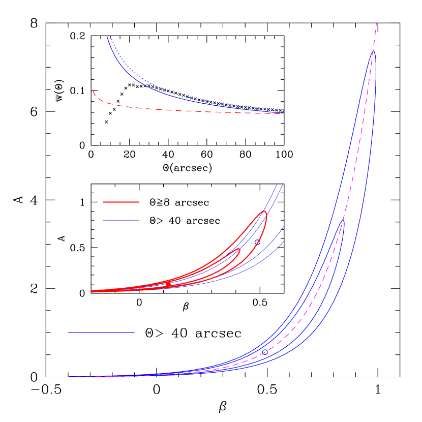
Figure 7: Contour levels of the $\chi^{2}$ function obtained by fitting a power-law model, $A\Theta^{-\beta}$, to the observed function $\bar{w}(\Theta)$ without correcting the data for the bias of the correlation estimator. The main body of the figure refers to the data at $\Theta>40$ arcsec. The open circle marks the position corresponding to the minimum value of the $\chi^{2}$ function. The continuous lines show the levels $\Delta\chi^{2}=2.30$ and $\Delta\chi^{2}=6.17$, which, for Gaussian residuals, correspond to the joint 68.3% and 95.4% confidence levels, respectively. The dashed line shows the function in equation 13. Bottom inset: The contours of the main panel are compared with those obtained from the data with $\Theta\geq 8$ arcsec. The levels $\Delta\chi^{2}=2.30$ and $\Delta\chi^{2}=6.17$ are marked by the heavy lines, while the parameters for the best-fitting model are denoted by a filled circle. Top inset: the measured correlation function (crosses) is compared with the best-fitting models at $\Theta>40$ arcsec with correlated errors (continuous line), and independent errors (dotted line). The best-fitting model for $\Theta\geq 8$ arcsec is marked by a dashed line.

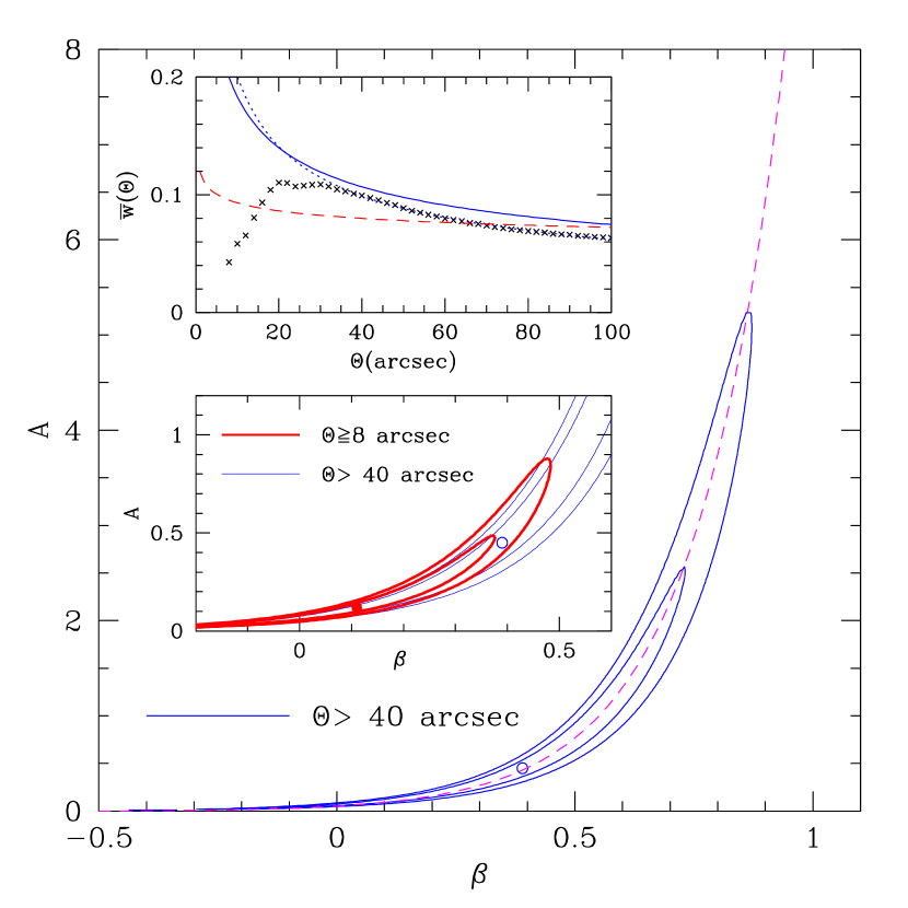
Figure 8: As in Figure 7 but for the bias-corrected data. The dashed line shows the function in equation 14.

An important result from the counts–in–cells analysis is that for $\Theta>40$ arcsec the correlation function of LBGs is very well described by a power–law model. While our data do not constrain separately the values of the parameters $A$ and $\beta$ with great accuracy, we find that the value $A^{\beta}$ is reasonably well determined. As the figures 7 and 8 show, $A$ and $\beta$ are strongly covariant, and regions of the plane with constant $\chi^{2}$ value are rather elongated and nearly unidimensional. When the data are not corrected for the bias of $\hat{\bar{w}}$, taking the analysis with 4 principal components as a reference case, we find that (for $\beta>0)$ these constant $\chi^{2}$ regions are centered around the line of equation,

$$A\simeq 0.62\,(0.49+\beta)^{3.8+2.7\,\beta}\;,$$ (13)

with a relatively small scatter. For bias corrected data, this becomes

$$A\simeq 0.56\,(0.56+\beta)^{4.1+2.6\,\beta}\;.$$ (14)

The ranges of variability for the single parameters $A$ and $\beta$ can be determined by projecting the curve corresponding to $\Delta\chi^{2}=1$ onto their axes. For the raw data, we find $\beta=0.50^{+0.25}_{-0.50}$, while allowing for for the bias of the correlation estimator corresponds to a slightly shallower slope, namely $\beta=0.40^{+0.25}_{-0.40}$. The amplitude of the best–fitting power–law model is even less precisely determined than the slope: when we do not correct for the bias we obtain $A=0.6^{+1.6}_{-0.6}$ arcsec^β, while when we account for $b_{\hat{\bar{w}}}$ we get $A=0.4^{+1.2}_{-0.4}$ arcsec^β. This difference, however, is significantly smaller than the error bar relative to $A$. It is also interesting that the corresponding best–fitting curves lie on opposite sides with respect to the data (see Figures 7 and 8). As we shall see is Section 8, the preferred values for $A$ and $\beta$ imply, through Limber deprojection, a strong spatial clustering, with a correlation length $r_{0}$ of a few Megaparsecs, in agreement with previous estimates by G98. Note that, before computing the best-fitting power–law models, we did not correct the data for the dilution of clustering caused by the residual contamination by stars in the galaxy catalogues, since this is negligible with respect to the overall uncertainty in the amplitude of the correlation function.

An intriguing result of our analysis is that the best power–law fit at $\Theta\lower 2.15277pt\hbox{$\;\buildrel>\over{\sim}\;$}40$ arcsec does not seem to describe well the average correlation function at smaller scales. Using the analysis with 4 principal components as a reference case, the best–model for $\Theta>40$ arcsec corresponds to $\Delta\chi^{2}=\chi^{2}-\chi^{2}_{\rm min}=2.73$ at $\Theta\geq 20$ arcsec, and to $\Delta\chi^{2}=5.95$ at $\Theta\geq 8$ arcsec . Taking these results at face value, it seems unlikely that our data are a realization of a point process with $\bar{w}=A\Theta^{-\beta}$ and $\beta\sim 0.5$ on scales $\Theta<40$ arcsec. As shown in the Figures 7 and 8, there is a relatively narrow region of the parameter space in which the value of $\Delta\chi^{2}$ for a power-law model is acceptable both for $\Theta>40$ arcsec and $\Theta\geq 8$ arcsec. Thus, we cannot rule out the possibility that the apparent break in the correlation function is just due to a statistical fluctuation. However, in this case, $\chi^{2}_{\rm min}/{\rm d.o.f.}>1$ for $\Theta\geq 8$ arcsec, making a single power–law over the whole range of angular separations an unlikely model, while the power–law fit is excellent for $\Theta>40$ arcsec. We will describe in moment a series of additional tests that we have performed to quantify the statistical significance of the observed behaviour of $\bar{w}(\Theta)$ at small scales.

5 THE SMALL–SCALE “BREAK”

There are three possible areas where we can look for the cause of a spurious “break” in the correlation function at small separations, namely biased data acquisition or reduction, systematic errors in the estimate of $\bar{w}$, and statistical fluctuations (e.g. due to shot noise or cosmic variance). This section is devoted to a discussion of these issues.

We can think of no obvious ways to introduce an artificial small–scale break in an otherwise correlated distribution of galaxies as a result of systematics during the observations and data reduction. This would require missing from an angular sample pairs of galaxies separated by $\sim 30$ arcsec or less, a scale which is about a factor of 20 or more smaller than the size of the fields we have observed, and a factor of $\sim 20$ larger than the typical isophotal size of a LBG. As discussed by G98, it is possible that the data are affected by slight variations of sensitivity from field to field and across the fields, with the central part being slightly deeper than the edges. Field to field variations would introduce a bias similar to the integral constraint, but they would not change the shape of the correlation function at small scales, in particular mimicking the break. Intra field variations would artificially increase the whole clustering signal over scales of the order of a few arcmin, but they would not affect it only at small scale.

It also seems unlikely that the break is an artifact of the data analysis. The most likely phase of the galaxy detection algorithm when systematics could be introduced is during the splitting of sources with blended isophotes. An improper splitting can potentially lead to underestimate the correlation function at very small angular separation if close pairs of galaxies are recorded as single objects by the detection software. We can estimate how many pairs could be potentially affected by undersplitting in our sample. For small angular separations, and assuming a power-law model $w(\theta)=A_{w}\theta^{-\beta}$ (with $\beta<2$), the number of expected pairs separated by less than $\theta$ is

$$N_{\rm pairs}(<\theta)\simeq\frac{1}{2}\,N_{\rm g}\,{\cal N}\,2\pi\int_{0}^{\theta}\theta^{\prime}\left[1+w(\theta^{\prime})\right]d\theta^{\prime}=\frac{1}{2}\,N_{g}\,{\cal N}\,\pi\theta^{2}\left[1+\frac{2A_{w}}{(2-\beta)\,\theta^{\beta}}\right]\;,$$ (15)

where ${\cal N}$ is the average surface density of LBGs, and $N_{\rm g}$ the total number of galaxies in our sample. Since the typical isophotal size of LBGs in the images is in the range $1<\Delta\theta<2$ arcsec, we expect than only pairs with $\theta<3$–4 arcsec can be mistakenly considered as single objects. For the best fitting power–law to our data at $\Theta>40$ arcsec, we find $N_{\rm pairs}(<4\,\,{\rm arcsec})\simeq 11.4$, comparable to 8 such close pairs observed in the real sample and suggesting that undersplitting is unlikely to be a factor in our sample. To quantify the effect of undersplitting, we have used a set of mock galaxy samples extracted from a correlated distribution with no break in the correlation function and artificially merged close pairs. These samples have the same average surface density and two–point correlation function (with no break at small scales) of the real LBGs (see Section 5.1 for details). Surprisingly, after merging all the pairs with angular separations $\theta<4$ arcsec, we found that the estimated values for $\bar{w}(\Theta)$ at $8\lower 2.15277pt\hbox{$\;\buildrel<\over{\sim}\;$}\Theta\lower 2.15277pt\hbox{$\;\buildrel<\over{\sim}\;$}40$ arcsec are actually larger than before. This is a consequence of the complex interplay between clustering and shot noise. What happens is that for $\Theta\geq 8$ arcsec, the second moment of the counts $\langle N^{2}\rangle$ is nearly unaffected by the merging of the close pairs, while $\langle N\rangle$ decreases by a factor $1+f_{\rm crowd}$, with $f_{\rm crowd}\ll 1$. Hence, the term $\langle N^{2}\rangle/\langle N\rangle^{2}$ increases by a factor $\sim 1+2\,f_{\rm crowd}$, while the shot noise term $1/\langle N\rangle$ increases only by a factor $\sim 1+f_{crowd}$. The net result is that the observed correlation function at $\Theta\lower 2.15277pt\hbox{$\;\buildrel<\over{\sim}\;$}8$ arcsec increases. In other words, since the average of the correlation function over the sample must vanish, imposing $w=-1$ at small separations corresponds to increasing its value at larger $\theta$. This shows that crowded isophotes cannot be the cause of the detected break in $\hat{\bar{w}}$.

Systematic errors could also have been introduced during the measure of the correlation function. An important test to carry out when assessing the significance of the break is to check if it is at all possible, with our data set, to detect in a statistically significant way deviations of the CPDF measured at small scales from a Poisson distribution. That this can be done is not obvious, since at $\Theta=8$ arcsec, $\langle N\rangle\simeq 0.07$, and the shot–noise contribution dominates the variance of the CPDF. Even if the large number of cells used in our analysis guarantees an optimal shot–noise subtraction (and the results of the maximum likelihood analysis presented in Section 3.4 agree with this expectation), it is possible that the break is simply the result of the inability to measure $\bar{w}(\Theta)$ at scales where the signal–to–noise is low . We carried out both the Kolmogorov–Smirnov and the Cramer–Smirnov–Von Mises (e.g. Eadie et al. 1971) tests and found that only at $\Theta\leq 10$ arcsec our data are compatible with being a random sampling from a Poisson distribution to the $95$% confidence level. In the interval $10\lower 2.15277pt\hbox{$\;\buildrel<\over{\sim}\;$}\Theta\lower 2.15277pt\hbox{$\;\buildrel<\over{\sim}\;$}30$ arcsec the data are significantly more clustered that the Poisson case, although less clustered than the extrapolation to small scales of the power law fit at $\Theta\lower 2.15277pt\hbox{$\;\buildrel<\over{\sim}\;$}30$ arcsec. Finally, we have also tested the stability of the break against artificially diluting our samples by a factor 4/3 and 2. Since shot noise is inversely proportional to the average density in the catalogue [see equation (A-4)], whenever discreteness effects are not subtracted correctly, changing the sampling rate introduces a bias in the estimate of $\bar{w}$. We noticed no significant change in the shape of $\bar{w}$ averaging over 20 different sparse sampled realizations. As a further test, we have also split our catalogue into two sub–samples and repeated the measure of $\bar{w}(\Theta)$ in each of them. We took one sub–sample to be the Westphal catalogue, and the other sub–sample the remainder of the fields. We measured $\bar{w}(\Theta)$ with the same techniques described above. As shown in the inset of Figure 2, we found that the correlation function of each sub–samples is characterized by a small–scale break similar to that of the whole sample, suggesting that it is not the result of statistical fluctuations, but it is a real feature of our sample.

5.1 Mock Catalogues

If the break is not the result of an improper measure (i.e. if it is present in our sample), that still does not mean that it reflects the clustering properties of the parent distribution, of which our galaxy fields are realizations. Since our sample of LBGs is relatively small, it could be, for example, that it is not representative of the parent distribution, and that the small–scale break is simply the result of normal fluctuations for the particular intrinsic clustering properties. In this section, we use numerical simulations to estimate the likelihood for this to occur.

Specifically, we measure $\bar{w}(\Theta)$ (with the method of the factorial moments) from a large number of realizations of a point process which has the same large–scale clustering properties of the LBGs but no small–scale break to estimate the probability to detect a significant deficit of close pairs in an artificial sample similar to the real one. We generate the mock LBG samples from a lognormal random field that has intrinsic $\bar{w}(\Theta)$ equal to the best power–law fit to the data for $\Theta>40$ arcsec, namely $\bar{w}(\Theta)=0.65/\Theta^{0.51}$, which is obtained assuming independent errors, and lies on top of the data points (note that using the other fitting functions discussed in Section 4 produces similar results). We generate the fields over a grid with physical size of $3600\times 3600$ arcsec² and grid step of 1.76 arcsec, smaller than the minimum distance between observed LBGs (1.92 arcsec). We subsequently extract the point sample by performing a Poisson sampling of the density field (see Appendix A). We assign a probability of finding “galaxies” at any given location as proportional to the intensity of the density field in that point, and we normalize it to obtain a distribution which has the same average density as the observed sample of LBGs. In this way, both the large–scale two point correlations and the surface density of objects are the same as those estimated from the galaxy sample (note that a grid point can host more than one galaxy). We generate eight different realizations of the field to extract eight samples of objects identical in shape and dimensions to the LBGs ones. We then estimate $\bar{w}$ from these mock catalogues by computing the factorial moments of the CDPF. The process is then repeated 1100 times to simulate the “cosmic variance”.

The results of the simulations are summarized in Figure 9, where the first two moments of the distribution of $\hat{\bar{w}}$ over the 1100 realizations are compared with the correlation function of the population. Note that the average correlation, $\langle\hat{\bar{w}}\rangle_{\rm mock}$, decreases monotonically with $\Theta$ on all scales. The cosmic bias is always negative, and, on large scales, comparable with the cosmic error. What do the simulations say about the statistical significance of the observed break? The probability distribution of $\hat{\bar{w}}(\Theta=10\,\,{\rm arcsec})$ over the 1100 realizations of the mock galaxy samples (Figure 10) shows that only in the 13% of the cases the measured correlation is smaller than the observed value, $\bar{w}_{\rm obs}$. This, however, does not quantify the significance of the break. Since data points at different angular separations are strongly correlated, in those realizations where galaxy correlations at $\Theta=10$ arcsec are feeble, $\hat{\bar{w}}$ tends to assume values that are smaller than the population value at every $\Theta$. For example, for $\Theta\geq 30$ arcsec, we find that only $\sim 10$% of these realizations have also $\hat{\bar{w}}\geq\bar{w}_{\rm obs}$. In other words, $\bar{w}(\Theta)$ of these samples does not show a break, it simply is small. What we need to test is how often a deviation from a smooth, power–law like behaviour is encountered, namely how often a correlation function which is monotonically decreasing with $\Theta$ on large scales changes its behaviour on small ones.

To test the shape of the correlation, we have used a non-parametric statistics as follows. First, for a given realization, we rank the values of $\hat{\bar{w}}(\Theta_{i})$ in order of increasing cell size $\Theta_{i}$. Subsequently, we generate a new set of ranks by sorting the values of $\hat{\bar{w}}(\Theta_{i})$ from the largest to the smallest. For a monotonically decreasing function, like a power–law with $\beta>0$, the two ranks coincide for every $\Theta_{i}$. In general, however, the correlation function evaluated at a given $\Theta_{i}$ will get different ranks in the two ordering schemes. This difference can be quantified using tests suited to compare sets of ordinal numbers, like the Spearman or Kendall rank correlation coefficients (Kendall & Stuart 1969). Finally, in order to find how many mock catalogues show a break in the small-scale correlation function, we looked for those realizations that have the same rank correlation coefficient of the observed data at $\Theta>30$ arcsec (which is 1, indicating perfect agreement between the two sets of ranks), and a rank correlation coefficient smaller or equal to that of the data at $\Theta\leq 30$ arcsec. Since we are interested in the global behaviour of the correlation function, to avoid local fluctuations, we considered only 10 values of $\Theta$, linearly equispaced between 10 and 100 arcsec. Independently of the correlation coefficient used, we found that these requirements are realized by $\sim 11\%$ of the realizations. Visual inspection has been used to check that, for the selected realizations, $\hat{\bar{w}}(\Theta)$ indeed showed a small-scale break.

Thus, the simulations show that if the population of LBGs is clustered at all scales with a correlation function similar to the best fitting power–law at $\Theta\geq 40$ arcsec, fluctuations produce a break similar to the observed one in $\sim 11$% of the cases. Such a confidence level is not high enough to conclude that the break is a true feature of the clustering properties of LBGs and not due to statistical fluctuations. However, it is not small enough to reject its detection with any confidence, either. Clearly, the reality of the break needs to be investigated with larger samples.

Other interesting conclusions can be drawn from the analysis of the mock catalogues. For instance, we can test the accuracy of the blockwise bootstrap method in estimating the variance and the bias of $\hat{\bar{w}}$. The comparison of the scatter of $\hat{\bar{w}}$ in the mock samples with that in the bootstrap realizations discussed in Section 3.2, shows that at worst they differ by $\sim 30$–40% on intermediate scales ($20\mathrel{\hbox to0.0pt{\lower 3.0pt\hbox{$\mathchar 536\relax$}\hss}\raise 2.0pt\hbox{$\mathchar 316\relax$}}\Theta\mathrel{\hbox to0.0pt{\lower 3.0pt\hbox{$\mathchar 536\relax$}\hss}\raise 2.0pt\hbox{$\mathchar 316\relax$}}60$ arcsec), with the bootstrap errors being larger. Note, however, that cosmic errors for $\hat{\bar{w}}$ depend on the three and four-point correlation functions, and these are different in the mock and real catalogues. Moreover, the bootstrap analysis includes also field–to–field variations that are not present in the mock catalogues. For this reason, to assess the quality of our method for estimating the errors in the correlation function, it would be preferable to compare bootstrap and true errors of the same point process. To do this, we pick up a mock realization at random, perform a bootstrap analysis on it, and compare the results with the true scatter among the 1100 mock realizations. We find that the size of bootstrap errors depend on the realization from which they have been generated. If its correlation function is strongly biased low with respect to the population value, the bootstrap errors tend to underestimate the uncertainties in $\hat{\bar{w}}$ by 40–50%. On the other hand, if the realization which has been bootstrapped shows particularly strong correlations, bootstrap errors will be overestimated. On average, we find that bootstrap errors are very reliable even though they tend to slightly underestimate the uncertainty in $\hat{\bar{w}}$. At the opposite, the bias of $\hat{\bar{w}}$ can be underestimated by a factor as large as $\sim 1.5$ using the bootstrap method.

We have also used the simulations to study how the PDF of the correlation estimator changes with the cell scale (see Szapudi et al. 2000 for a similar analysis in three dimensions). Accurate modeling of this would be extremely important for developing robust maximum likelihood methods. In Figure 12, we plot the PDF of $\hat{\bar{w}}$ for cells with $\Theta=10$ arcsec and $\Theta=100$ arcsec. To facilitate the comparison of the distributions, we plot them as functions of the normalized residuals $\Delta\bar{w}=(\hat{\bar{w}}-\langle\hat{\bar{w}}\rangle)/\sigma_{\hat{\bar{w}}}$, where $\sigma_{\hat{\bar{w}}}$ denotes the r.m.s. value of $\hat{\bar{w}}-\langle\hat{\bar{w}}\rangle$. In this way, both the probability distributions have vanishing mean and unitary variance. As expected, these distributions are positively skewed. However, the cosmic bias is always negative, meaning that it is more likely to underestimate the correlation function than to overestimate it. It is interesting to note that the skewness of these PDFs markedly increases when going from $\Theta=10$ arcsec (where shot–noise dominates the variance of the CIC) to $\Theta=100$ arcsec (where finite volume effects are the major source of uncertainty).

6 ARE CURRENT SAMPLES REPRESENTATIVE OF THE LBG POPULATION?

In this section, we consider the problem of whether or not the current samples provide a fair representation of the clustering properties of LBGs. For our purposes, a galaxy sample is “fair” if the correlation function measured from it differs from the population value by less than a specified (usually small) amount, within a reasonable confidence level. The analysis of the mock catalogs is very useful to gain some insight into this problem. The simulations show that if the true clustering strength of LBGs is as strong as the one that we have measured, then we should expect correlation estimates extracted from samples similar in size and geometry to ours to be significantly biased. In addition, the cosmic scatter between the measures obtained from different samples should be large. For example, Figure 11 shows that the probability that the measure of $\bar{w}(\Theta)$ from a sample with the size of our dataset differs from the population value by less than 20% is 34% and 25% for $\Theta=50$ and 100 arcsec, respectively. It also shows that the estimated value of $\bar{w}$ at $\Theta=50$ ($100$) arcsec is underestimated by more than a factor of 2 in the 21% (35 %) of the cases, while the probability of overestimating the correlation function by more than a factor 1.5 is instead very small, namely, 4% and 3% for $\Theta=50$ and 100 arcsec. This is consistent with the fact that the variance of $\hat{\bar{w}}$ on these scales is comparable with the observed correlation $\bar{w}_{\rm obs}$ (see Figure 9). The situation is worsened by the fact that also the bias of the estimator of the correlation function is of the same order of magnitude of $\bar{w}_{\rm obs}$, at least on large scales. Note also that the true bias is likely to be larger than the value derived from the simulations, because the intrinsic clustering strength of the galaxies is likely to be larger than the value used in the simulations. The fluctuations on the scales of our sample, therefore, will be larger.

Two conclusions emerge from this discussion. Firstly, it is clear that much larger samples are needed to obtain precision measures of the correlation function of LBGs. Secondly, the simulations show that the direction of the bias that affect the available samples is such that the clustering strength of LBGs is probably underestimated by the current measures. Thus, the conclusion that these sources are strongly clustered in space (as we shall quantify later) is very likely a robust statement.

7 THE CORRELATION FUNCTION FROM PAIR COUNTS

As a final check, and to understand the stability of our results with the method of analysis, we re-computed the angular correlation function of LBGs using a different set of estimators, not involving CIC. Specifically, we have measured the function $\widetilde{w}(\theta)$, defined as the fractional excess of LBG pairs at angular separations smaller than $\theta$ over the expectations from the Poisson distribution. This is expressed in terms of the two–point function $w(\theta)$ as

$$\widetilde{w}(\theta)=\frac{\displaystyle{\int_{0}^{\theta}\phi(\theta^{\prime})\,w(\theta^{\prime})\,d\theta^{\prime}}}{\displaystyle{\int_{0}^{\theta}\phi(\theta^{\prime})\,d\theta^{\prime}}}=\int_{0}^{\theta}\psi(\theta^{\prime})\,w(\theta^{\prime})\,d\theta^{\prime}\;,$$ (16)

where $\phi(\theta)$ is a weighting function which depends on the geometry of the sample as,

$$\phi(\theta)=\sum_{i}\int_{\Sigma_{i}}d\Omega_{1}\int_{\Sigma_{i}}d\Omega_{2}\,\delta_{D}(|\theta_{2}-\theta_{1}|)$$ (17)

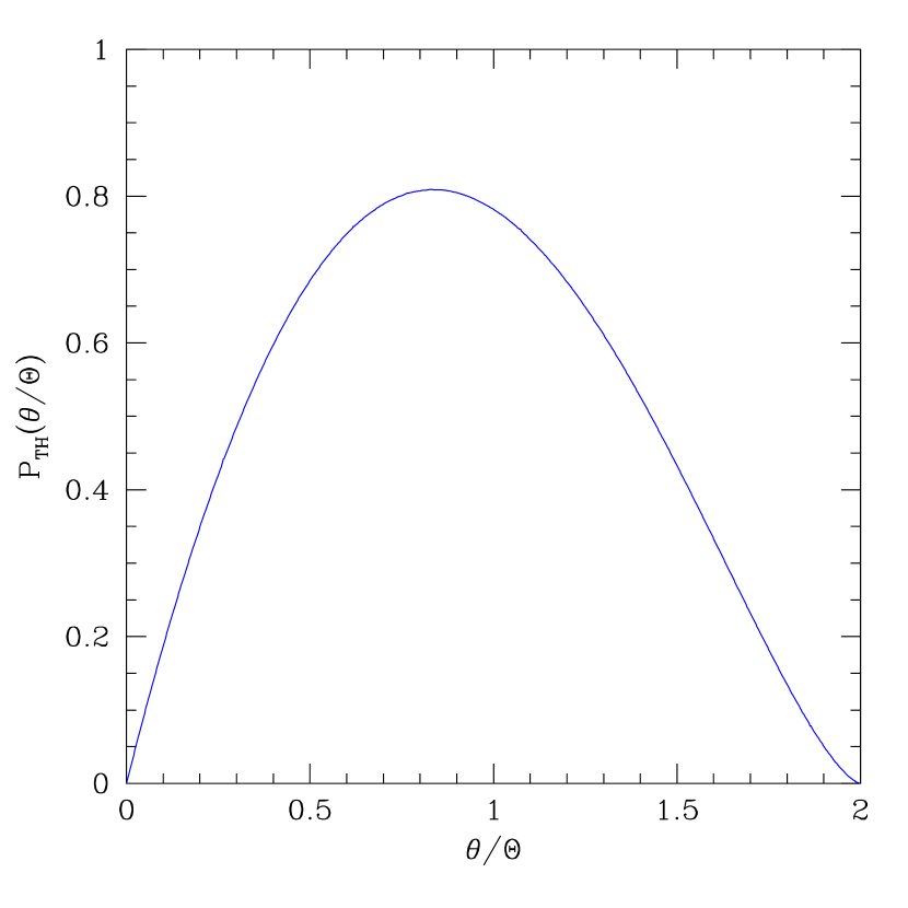
Figure B1: Distribution function of the normalized angular separations, $\theta/\Theta$, between points lying within a circular cell of radius $\Theta$. The analytic expression of this function is given in equation (B-10).

($\delta_{D}$ is the Dirac delta distribution, and the index $i$ runs over the different LBG fields). The function $\phi(\theta)$ can be determined by Monte Carlo integration. For our sample, the normalized distribution $\psi$ is very similar to the function given in equation B-10 (and shown in Figure B1) with $\Theta\sim 360$ arcsec, but has an extended tail at large angular separations (i.e. for $\theta>500$ arcsec). For angles much smaller than the sample size, $\phi\simeq 2\pi\theta$, and $\psi\simeq 2\theta$, and assuming $w(\theta)=A_{w}\theta^{-\beta}$ with $\beta<2$, one finds $\widetilde{w}(\theta)\simeq[2A_{w}/(2-\beta)]\theta^{-\beta}$. However, since in any finite sample there are less pairs of galaxies with separation equal to $\theta$ than in the projected sphere, $\widetilde{w}(\theta)$ will soon depart from its asymptotic behaviour, and, if $\beta>0$, it will assume larger values. This means that, if $w(\theta)$ is a power–law, $\widetilde{w}(\theta)$ is not, while $\bar{w}(\Theta)$ is. This is one of the reasons why we have used $\bar{w}$ as our primary statistics. Useful information, however, are obtained from $\widetilde{w}(\theta)$, as we will show in a moment.

A number of estimators of $\widetilde{w}(\theta)$ have been proposed. These account for boundary effects and the geometry of the sample by comparing the distribution of the angular separations between the galaxies to that of a high–density Poisson process covering the sample area. We used the three estimators

$$\hat{\widetilde{w}}_{1} = \frac{DD}{DR}-1$$ (18)

$$\hat{\widetilde{w}}_{2} = \frac{DD-2DR+RR}{RR}$$ (19)

$$\hat{\widetilde{w}}_{3} = \frac{DD\cdot RR}{DR^{2}}-1$$ (20)

proposed by Peebles (1980), Landy & Szalay (1993), and Hamilton (1993) respectively, where $DD$, $DR$, and $RR$ are the fractions of (distinct) data–data, data–random, random–random pairs with an angular separation smaller than $\theta$, suitably normalized. As in Section 3, in one case we computed $\widetilde{w}(\theta)$ by combining all the fields in a single sample (which minimizes the integral constraint bias); in another case, we took the average of the the measures from each single field (which minimizes spurious signals coming from field–to–field variations). For $\theta\mathrel{\hbox to0.0pt{\lower 3.0pt\hbox{$\mathchar 536\relax$}\hss}\raise 2.0pt\hbox{$\mathchar 316\relax$}}40$ arcsec, the values of $\widetilde{w}(\theta)$ from the two methods (for each estimator) differ at most by $\sim 0.05$, with the first method giving higher correlations as in the CIC analysis. The difference decreases with increasing $\theta$, becoming $\sim 0.01$ for $\theta\mathrel{\hbox to0.0pt{\lower 3.0pt\hbox{$\mathchar 536\relax$}\hss}\raise 2.0pt\hbox{$\mathchar 318\relax$}}100$ arcsec, suggesting that on large scales methods based on pair counts could be less affected by the integral constraint bias than CIC, perhaps because of they account for edge effects more effectively (see below).

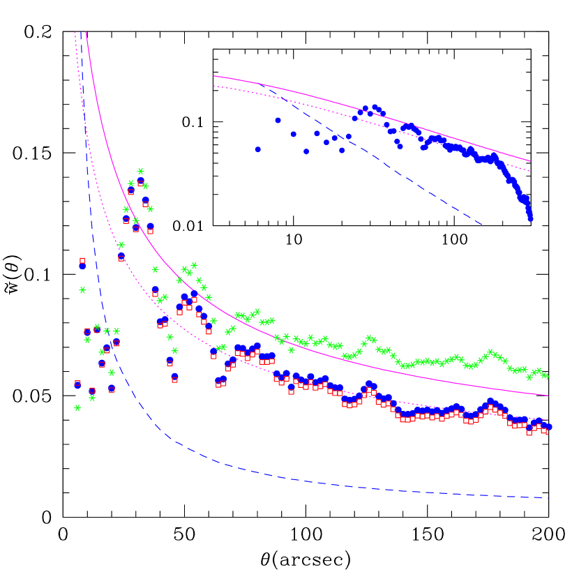
Figure 13: Average correlation function $\widetilde{w}(\theta)$ estimated from pair-counts. Filled dots, open squares and stars refer to the Landy & Szalay, Hamilton, and Peebles estimators, respectively. The dashed line marks the size of Poisson errors for the Landy & Szalay estimator. The continuous line shows the function $\widetilde{w}(\theta)$ corresponding to the power-law model $\bar{w}(\Theta)=0.65/\Theta^{0.51}$ (with $\Theta$ in arcsec) which approximates the results from the CIC analysis. The dotted line is obtained by multiplying the continuous curve by 0.8. The inset presents the results of the Landy & Szalay estimator in logarithmic space. The notation is as in the main panel.

Results obtained combining all the fields together are shown in Figure 13. The estimators by Hamilton (1993) and Landy & Szalay (1993) are in nearly perfect agreement, while $\hat{\widetilde{w}}_{1}$ gives stronger correlations on large scales. This latter estimator is subject to an uncertainty proportional to the error in the galaxy surface density, $\delta{\cal N}$ (e.g. Hamilton 1993). While this error tends to zero when a large number of catalogues is considered, the expectation value of $\widetilde{w}_{1}$ still differs from the true correlation. This bias, which is proportional to $\widetilde{w}$ evaluated on the scale of sample, scales like the variance of the errors in the galaxy surface density. On the other hand, $\hat{\widetilde{w}}_{2}$ and $\hat{\widetilde{w}}_{3}$ show fluctuations with respect to the expectation value which are proportional to $(\delta{\cal N})^{2}$, even when they are computed from the single fields. At separations which are small compared to the size of the single fields, the average over a large number of samples is affected by the same bias as $\hat{\widetilde{w}}_{1}$, while at large separations the precise form of the correction depends on the particular estimator used to measure the correlation function (Hamilton 1993; Landy & Szalay 1993; Maddox et al. 1996).

Essentially, $\bar{w}$ and $\widetilde{w}$ are averages of the same correlation function done with different weighting schemes. Specifically, $\bar{w}$ is obtained with a relatively wide smoothing kernel, while $\widetilde{w}$ is more sensible to local variations (at least for $\theta<300$ arcsec, where $\psi$ is increasing with $\theta$). Thus, $\bar{w}$ describes the global trend of the correlation function, while $\widetilde{w}$ emphasizes the scales at which large fluctuations with respect to the mean trend are found. This is useful, for instance, to study the clustering properties on very small scales, e.g. where $\bar{w}$ seems to depart from its smooth large–scale behaviour. This is illustrated in Figure 13, which shows that the pair–count statistics is in overall good agreement with the counts–in–cells analysis. On large scales, $\theta\mathrel{\hbox to0.0pt{\lower 3.0pt\hbox{$\mathchar 536\relax$}\hss}\raise 2.0pt\hbox{$\mathchar 318\relax$}}50$ arcsec, both $\hat{\widetilde{w}}_{2}$ and $\hat{\widetilde{w}}_{3}$ are well approximated by a power–law with slope $\beta\simeq 0.5$, while $\hat{\widetilde{w}}_{1}$ has a shallower one, $\beta\simeq 0.3$. The clustering amplitude from the CIC analysis is intermediate between the various pair–counts estimates. In particular, $\hat{\widetilde{w}}_{2}$ and $\hat{\widetilde{w}}_{3}$ are $\sim 20\%$ lower than the the CIC value (in agreement with the maximum likelihood analysis in Section 3.4.3), while $\hat{\widetilde{w}}_{1}$ is slightly higher. These differences reflect the magnitude with which the bias of the estimators affects the measures.

The function $\widetilde{w}(\theta)$ also shows a weaker clustering strength at small scales than the extrapolation of the corresponding large–scale fit, of similar statistical significance as the one observed for $\bar{w}(\Theta)$. For $\theta\mathrel{\hbox to0.0pt{\lower 3.0pt\hbox{$\mathchar 536\relax$}\hss}\raise 2.0pt\hbox{$\mathchar 316\relax$}}70$ arcsec, the correlation functions in Figure 13 show large oscillations relative to the fit at larger scales. A lack of galaxy pairs at $\theta\mathrel{\hbox to0.0pt{\lower 3.0pt\hbox{$\mathchar 536\relax$}\hss}\raise 2.0pt\hbox{$\mathchar 316\relax$}}25$ arcsec respect to the expectation from the same fit is observed as well. For example, there are 224 pairs of LBGs separated by less than 20 arcsec in our sample, while in absence of the break we would have expected $\sim 243.3$ pairs (this is obtained assuming $\bar{w}(\Theta)=0.65/\Theta^{0.51}$; if the galaxy correlation function is $20\%$ lower than the CIC results, $\sim 236.6$ pairs are expected). Since the measures of $\widetilde{w}(\theta)$ and $\bar{w}(\Theta)$ are differently affected by shot noise, we interpret this lack of small–scale signal in both statistics as an additional indication that the feature is due to a real lack of pairs with small angular separations in the data, albeit detected with low signal–to–noise ratio.

The function $\widetilde{w}$ is better suited than $\bar{w}(\Theta)$ to study the correlation function at large scales. When using the CIC, we avoided edge effects to contaminate the measure of $\bar{w}(\Theta)$ at large separations by considering only those cells that did not overlap with the boundaries of the samples, which implied some loss of information. On the contrary, all the galaxy–galaxy separations are used to estimate $\widetilde{w}$. Note that the relative weight of galaxies lying near the boundaries with respect to those sitting at the centre of a field increases with the angular separations. In particular, for separations much smaller than half the field size, objects at the edge have half the weight of those at the centre. The opposite situation is found for separations larger than half the sample size, where only objects at the edge can contribute. This suggests that large–scale correlations should be more reliably measured by $\widetilde{w}$ than by the CIC analysis. Using $\widetilde{w}$, we find that the correlation function of LBGs deviates from a power–law behaviour also at large scales ($\theta\mathrel{\hbox to0.0pt{\lower 3.0pt\hbox{$\mathchar 536\relax$}\hss}\raise 2.0pt\hbox{$\mathchar 318\relax$}}180$ arcsec, see the inset of Figure 13). This is evident with all the estimators we considered. However, we do not think that this feature is real. In fact, because of the integral constraint, we expect the estimated correlation function to oscillate around zero on scales comparable with the sample size. In correspondence of the first zero–crossing a sudden departure from any small–scale smooth behaviour is then expected. Since the break appears on a scale corresponding to one third of the linear size of our smallest fields, this could explain its presence. To test if the break is due to boundary effects of our estimators, we used the mock catalogues discussed in Section 5.1. We found that large-scale breaks similar to the observed one are quite common. Sometimes, adding a constant value to the correlation function is enough to restore the missing large-scale power. Note that the presence of this spurious break at $\theta\mathrel{\hbox to0.0pt{\lower 3.0pt\hbox{$\mathchar 536\relax$}\hss}\raise 2.0pt\hbox{$\mathchar 318\relax$}}180$ arcsec could explain the reason why G98 found a steeper correlation than reported here, since they considered all the data with angular separations $\theta<330$ arcsec to determine the best–fitting power–law.

8 DISCUSSION

One of the motivations that led us to revisit the measure of the angular correlation function of LBGs was to test the robustness of the previous results, namely that these galaxies are characterized by strong spatial clustering, with a correlation length that rivals that of local galaxies. The new measure discussed here confirms this result, and also gives some insight on the shape of the correlation function. Interestingly, our error analysis shows that the conclusion that the clustering strength of $z\sim 3$ LBGs is larger than that of the mass for essentially all commonly adopted cosmological models holds (at the $3\sigma$ level), implying that these sources are highly biased tracers of the mass distribution.

We have used the Limber transform to derive from the $\bar{w}(\theta)$ both the spatial correlation length and the bias parameter in a set of reference cosmological scenarios. We considered a matter dominated, low–density universe (OCDM) with present–day mass density parameter $\Omega_{\rm M}=0.3$, vacuum density parameter $\Omega_{\Lambda}=0$ and Hubble constant $H_{0}=100\,h\,{\rm km\,s^{-1}\,Mpc^{-1}}$, with $h=0.7$; a flat, vacuum dominated, low–density universe ($\Lambda$CDM) with $\Omega_{\rm M}=0.3$, $\Omega_{\Lambda}=0.7$ and $h=0.7$; and an Einstein–de Sitter model ($\tau$CDM) with $\Omega_{\rm M}=1$, $\Omega_{\Lambda}=0$ and $h=0.5$. In all cases, we have assumed that the linear power spectrum of density perturbations approximates the cold dark matter (CDM) one with primordial spectral index $n=1$, transfer function by Bardeen et al (1986), and with spectral shape parameter $\Gamma=0.21$. The amplitude of the power spectrum is fixed to reproduce the observed abundance of rich galaxy clusters in the local universe (e.g. Eke et al. 1996; Jenkins et al. 1998).

To derive the bias parameter of the LBGs we first computed the non-linear autocorrelation of mass density fluctuations at redshift $z$, $\xi_{\rm m}(r,z)$ (with $r$ in comoving units), adopting the algorithm by Peacock & Dodds (1996). We then used the small angle version of the Limber equation to calculate the angular correlation function of a set of objects which trace the mass density field, and are distributed in redshift like the LBGs, namely

$$w_{\rm m}(\theta)=\frac{\displaystyle{\int_{0}^{\infty}dz\,N^{2}(z)\int_{-\infty}^{\infty}[dx/R_{\rm H}(z)]\,\xi_{\rm m}\left\{\sqrt{[D_{\rm M}(z)\theta]^{2}+x^{2}},z\right\}}}{\displaystyle{\left[\int dz\,N(z)\right]^{2}}}\;,$$ (21)

with $N(z)\,dz$ the galaxy number counts in the redshift shell $z,z+dz$, $D_{\rm M}(z)$ the proper motion distance (known also as the transverse comoving diameter distance), and $R_{\rm H}(z)$ the Hubble radius at redshift $z$,

$$R_{\rm H}(z)=\frac{c}{H_{0}}(1+z)^{-1}\left\{1+\Omega_{0}z+\Omega_{\Lambda}\left[\frac{1}{(1+z)^{2}}-1\right]\right\}^{-1/2}\;.$$ (22)

This assumes that: i) $\theta\ll 1$ (with $\theta$ in radians); ii) the spatial correlation length ($r_{0}(z)$, such that $\xi[r_{0}(z),z]=1$) is much smaller than the depth of the survey; iii) the thickness of the comoving shell in which $N\neq 0$ is comparable with the depth of the survey. All these requirements are satisfied for both the LBGs and the mass distribution. We derived $N(z)$ from the redshift distribution presented by Giavalisco & Dickinson (2001), which includes 546 spectroscopic redshifts, and interpolated the histogram of redshifts with a cubic spline. Finally, we computed $\bar{w}_{\rm m}(\Theta)$ by averaging $w_{\rm m}(\theta)$ over the distribution of angular separations corresponding to a circular cell (see equation (B-10) and Figure B1). The effective bias parameter, $b_{\rm eff}$, is defined as $b^{2}_{\rm eff}(\Theta)=\bar{w}(\Theta)/\bar{w}_{\rm m}(\Theta)$, and we computed it in the same range of $\Theta$ where we studied $\bar{w}(\Theta)$. The effective bias as a function of the angular separation is plotted in Figure 14, which shows that independently of the underlying cosmological parameters, LBGs are strongly biased tracers of the mass distribution if this is similar to the CDM one. Moreover, for $\Theta>30$ arcsec, $b_{\rm eff}$ shows little evolution with $\Theta$. Choosing $\Theta=60$ arcsec as a reference case, from the raw data we find

$$b_{\rm eff}=2.2^{+0.5}_{-0.5},\,\,\,\,\,\,\,\,\,\,2.8^{+0.5}_{-0.6},\,\,\,\,\,\,\,\,\,\,3.9^{+0.8}_{-0.9}\;,$$

for OCDM, $\Lambda$CDM and $\tau$CDM, respectively. Correcting for the bias of the estimator, one gets

$$b_{\rm eff}=2.4^{+0.4}_{-0.5},\,\,\,\,\,\,\,\,\,\,3.0^{+0.5}_{-0.6},\,\,\,\,\,\,\,\,\,\,4.2^{+0.7}_{-0.8}\;,$$

in the three cases.

The Limber equation can also be used to deproject the observed angular correlation function and derive the spatial correlation length, $r_{0}$, of LBGs. For this calculation, we have neglected the possibility of the presence of a small–scale break in the two–point correlation function of LBGs, and used the best-fitting power–law model of the data at $\Theta>40$ arcsec as representative of the clustering properties of the population. The function $w(\theta)$ has been obtained using equation (B-7) in Appendix B. Note that we have assumed that the power–law model that describes the data at $\Theta\leq 100$ arcsec still provides a good approximation to the angular correlation function on scales which have not been tested by the observations. In principle, this (unavoidable) extrapolation could introduce strong systematic errors in the measure of the spatial correlation length. However, the observed scatter in the galaxy number density between the fields is compatible with this hypothesis (see Section 3.3). In this case, also the spatial correlation function, $\xi(r,z)$, is described by a power–law. In particular, if the redshift dependence of this function can be factorized as $\xi(r,z)=F(z)\,(r/r_{0})^{-\gamma}$, then, the corresponding $w(\theta)$ has the form $w(\theta)=A_{w}\theta^{-\beta}$, where $\beta=\gamma-1$ with

$$A_{w}=r_{0}^{\gamma}\,\sqrt{\pi}\,\frac{\Gamma[(\gamma-1)/2]}{\Gamma(\gamma/2)}\,\frac{\displaystyle{\int_{0}^{\infty}[dz/R_{\rm H}(z)]\,F(z)\,D_{\rm M}^{1-\gamma}(z)\,N^{2}(z)}}{\displaystyle{\left[\int_{0}^{\infty}N(z)\,dz\right]^{2}}}\;,$$ (23)

(Totsuji & Kihara 1969; Peebles 1980). The function $F(z)$ is not known, but in the case of LBGs this is not a limitation, since the corresponding distribution of cosmic time is considerably narrower (and more peaked) than that of traditional flux–limited redshift surveys, and little evolution of their clustering strength is expected over such a narrow range of cosmic time. In this case, the function $F(z)$ can be taken out of the integral in equation 23, and the quantity $r_{0}(z)=r_{0}[F(z)]^{1/\gamma}$ is the correlation length at the epoch of the observations. We have verified this approximation by considering the three cases of fixed clustering pattern in proper coordinates ($F(z)\propto(1+z)^{-(3-\gamma)}$), linearly growing clustering ($F(z)\propto D_{+}^{2}(z)$, with $D_{+}(z)$ the growth factor of linear density fluctuations), and fixed clustering pattern in comoving coordinates ($F(z)={\rm const}$). Using these approximations returns values for $r_{0}$ which differ by a few parts in a thousand.

Adopting the power–law models obtained using 4 principal components of the bootstrap errors to fit the raw data, we find:

$$r_{0}=3.5^{+1.0}_{-1.3}\,h^{-1}{\rm\,Mpc};\hbox{~{}~{}~{}~{}~{}}4.1^{+1.0}_{-1.5}\,h^{-1}{\rm\,Mpc};\hbox{~{}~{}~{}~{}~{}}2.4^{+0.7}_{-0.9}\,h^{-1}{\rm\,Mpc},$$

for OCDM, $\Lambda$CDM and $\tau$CDM, respectively. Correcting for the bias of the correlation estimator, one gets

$$r_{0}=3.9^{+1.1}_{-1.7}\,h^{-1}{\rm\,Mpc};\hbox{~{}~{}~{}~{}~{}}4.6^{+1.2}_{-2.0}\,h^{-1}{\rm\,Mpc};\hbox{~{}~{}~{}~{}~{}}2.7^{+0.8}_{-1.2}\,h^{-1}{\rm\,Mpc}.$$

The errorbars have been determined as follows. We assumed Gaussian residuals for the principal component analysis presented in Section 4 so that each point in the parameter space can be associated with a probability through the $\chi^{2}$ function. An histogram of $r_{0}$ values has then been constructed, mapping the parameter space and using the $\chi^{2}$ probabilities as weights. The 95% confidence level around the most probable value (determined by locating the $2.5$ and $97.5$ percentiles) has been taken as the uncertainty for $r_{0}$. Note that, the most probable values tend to be slightly higher than those presented above (we get $r_{0}=3.8,\,4.3,\,2.6\,h^{-1}{\rm\,Mpc}$ and $r_{0}=4.4,\,5.1,\,3.0\,h^{-1}{\rm\,Mpc}$ for the raw and bias corrected data, respectively). We preferred to quote the correlation length corresponding to the best–fitting power–law model since this is not affected by the assumption of Gaussian residuals. However, since $r_{0}$ is obtained with a non–linear transformation of the parameters $A$ and $\beta$, this could introduce some systematic error in the final estimates. When we do not correct for the bias of the estimator, our results are in very good agreement with G98. Thus, despite the CIC method yielded an angular correlation function which is shallower and with a smaller amplitude that that presented by G98, the implied correlation length seems to be robust. This is because the parameters of the power–law model are strongly covariant, and the comoving correlation length $r_{0}$ is much more tightly constrained than either $A$ or $\beta$ individually.

The interesting results of this study are that the correlation function of LBGs at $z\sim 3$ is very well approximated by a power–law at angular separations $40<\theta<180$ and, perhaps more importantly, that we confirm the strong spatial clustering, and hence implied large bias, reported in previous works (Steidel et al. 1998; G98; A98). The correlation length discussed here is somewhat smaller than that found by A98, who measured it using the counts–in–cells statistics in a three dimensional sample. Perhaps part of the difference can be explained by the possible presence of clustering segregation with the luminosity (Giavalisco & Dickinson 2001), since the spectroscopic sample considered by A98 is about 0.5 magnitudes brighter than the pure photometric samples used here and by G98. More likely the difference could be due to statistical fluctuations, since their sample is significantly smaller (in terms of number of galaxies) than the one discussed here and it includes less fields, making it more prone to cosmic variance effects. Redshift distortions, either due to peculiar motions or to uncertainties in the measure of the systemic redshifts of the galaxies (e.g. see Pettini et al. 2001) could also contribute to the observed discrepancy. We are currently investigating this possibility (Porciani & Giavalisco, in preparation). Note that our results for $b_{\rm eff}$ and $r_{0}$ might be biased towards high values if our sample is affected by significant field–to–field variations, while they might be biased towards low values if inter–field fluctuations are not important and the bootstrap method underestimates the bias of $\hat{\bar{w}}$.

The value of the slope of the correlation function is the main difference with the measure by G98, who report $\beta=0.98\pm 0.32$, somewhat larger than the value $0.50^{+0.25}_{-0.50}$ found here. This discrepancy could be a consequence of the wider range of angular separations considered by G98 for their power–law modeling of the data, i.e. $\theta\leq 330$ arcsec, in combination with the assumption that error bars at different angular separations are statistically independent. In fact, we found that the correlation function of LBGs has a large scale break at $\theta\mathrel{\hbox to0.0pt{\lower 3.0pt\hbox{$\mathchar 536\relax$}\hss}\raise 2.0pt\hbox{$\mathchar 318\relax$}}180$ arcsec probably due to the integral constraint bias. Note, however, that even though the best–fitting values for $\beta$ differ by a factor of 2, the $1\,\sigma$ errors significantly overlap. The result $\beta\sim 0.5$ is more in line with the values observed at intermediate redshift (Le Févre et al. 1996; Carlberg et al. 1997). This is an interesting and useful constraint to the models of galaxy formation.

The strong spatial clustering of LBGs suggests that they are associated with massive structures. In other words, to simultaneously reproduce the clustering strength and the spatial abundance of the LBGs in the framework of the cold dark matter model, their hosting dark matter halos must be relatively massive (e.g. see the discussion in G98; A98; Giavalisco & Dickinson 2001). Note that the individual galaxies need not coincide with the massive halos, but simply to trace their spatial position. For example, a strong clustering would also be observed in a scenario where LBGs are associated with sub–halos of low mass, which are satellites of massive ones (e.g. Kolatt et al. 1999; Wechsler et al. 2000). In this model, the sub–halos become active star formers, and thus observable, as a result of merging and interactions. Whatever the specific mechanism, it is important to realize that for strong clustering to be observable it is necessary that the galaxies that numerically dominate the sample must be associated with strongly clustered regions of the mass density field. An implication is that “field halos” of small mass (i.e. not associated with more massive ones), cannot significantly populate the samples, because they are much more numerous and less clustered than the observations would imply. Thus, as discussed in Giavalisco & Dickinson (2001), the clustering strength can be used, in conjunction with an assumed mass spectrum, to constrain the relationship between mass and UV luminosity.

An intriguing result of this study is the possibility that the correlation function has a break at small angular scales, $\Theta\lower 2.15277pt\hbox{$\;\buildrel<\over{\sim}\;$}30$ arcsec, where it seems to become smaller than the extrapolation of the power–law fitted at large scales. The $\chi^{2}$ test and the fact that the feature reproduces in each of the sub–samples if we split our LBG sample in two parts suggest that the break is real. On the other hand, the confidence level of the break detection taking the numerical simulations at face value is marginal, namely 90%, and more data are required to confirm it or reject it. It is nonetheless interesting to briefly discuss some of the implications.

A small–scale break means that there are too few pairs of galaxies luminous enough to be included in our sample that have angular separations smaller than $\sim 30$ arcsec, compared to the expectations of the power–law correlation function. This can occur, for example, if the substructure within the halos hosting the galaxies is such that only one galaxy per halo is, on average, bright enough to be detected by our survey (the presence of fainter galaxies is, of course, unconstrained). In this case the break is simply the result of the average size of the halos, namely of the fact that dark matter halos hosting LBGs have finite size and are mutually exclusive in space . At $z=3$, the scale of the break, say $\Theta_{\rm br}=25\pm 5$ arcsec, corresponds to a comoving size of $0.52\pm 0.10\,h^{-1}$ Mpc for OCDM, $0.54\pm 0.11\,h^{-1}$ Mpc ($\Lambda$CDM), and $0.36\pm 0.07\,h^{-1}$ Mpc ($\tau$CDM). Assuming that dark matter halos form from spherically symmetric density perturbations, and that their virialization epoch is twice the turnaround time, these lengths correspond to the diameters of objects with mass $2.1^{+1.5}_{-1.0}\times 10^{12}M_{\odot}$ (OCDM), $1.8^{+1.3}_{-0.9}\times 10^{12}M_{\odot}$ ($\Lambda$CDM), $2.5^{+1.7}_{-1.3}\times 10^{12}M_{\odot}$ ($\tau$CDM). Thus, the mass scale associated with the break is consistent with that of halos with mass and volume density required to reproduce the observed abundance and clustering strength (e.g. see Giavalisco & Dickinson 2001). Interestingly, these values are largely insensitive to the cosmology.

In view of the importance of the detection of the break as a possible indicator of the mass of the galaxies, we have compared the observed $\bar{w}(\Theta)$ to the prediction from the spatial exclusion model. We have assumed that there is only one visible LBG per dark matter halo, and that its position coincides with the “center” of the halo. Then, the correlation function of the galaxies coincides with that of the halos, and a simple model for their angular clustering, accounting for mutual exclusion, can be built as follows. We have also assumed that the cross–correlation function between halos of mass $M_{1}$ and $M_{2}$ at redshifts $z$ is given by

$$\xi_{\rm h}(r,M_{1},M_{2},z)=\begin{cases}{b(M_{1},z)b(M_{2},z)\,\xi_{\rm m}(r,z)},&\text{if $r>R_{1}+R_{2}$}\\ {-1},&\text{otherwise}\\ \end{cases}$$ (24)

where $b(M,z)$ is the linear bias parameter of dark matter halos of mass $M$ that have virialized at redshift $z$ (Mo & White 1996), and the Eulerian radii of the collapsed halos, $R_{1}$ and $R_{2}$, are determined assuming that halos originated from the collapse of spherically symmetric perturbations that virialized at the epoch corresponding to two turnaround times (e.g. Lacey & Cole 1993; Kochanek 1995; Bryan & Norman 1998). The mass density autocorrelation function, $\xi_{\rm m}(r,z)$ is computed using the method by Peacock & Dodds (1996), as described earlier. From that we have derived the halo correlation function using the Press–Schechter mass function $n(M,z)$ (Press & Schechter 1974) as

$$\xi_{\rm h}(r,z)=\frac{\displaystyle{\int dM_{1}\int dM_{2}\,n(M_{1},z)\,n(M_{2},z)\,\xi_{\rm h}(r,M_{1},M_{2},z)}}{\displaystyle{\left[\int dMn(M,z)\right]^{2}}}\;.$$ (25)

Finally, we have used the Limber equation in the small angle approximation to transform $\xi_{\rm h}$ into the angular correlation function of the halos (cf. Coles et al. 1998), and have calculated $\bar{w}(\Theta)$ using equations (B-8) and (B-10). Since our sample of LBGs is flux limited, we have considered mass–limited samples of halos in the calculation. Figure 15 shows the results obtained using dark matter halos with different mass thresholds compared to the observed correlation function in the $\Lambda$CDM cosmology. The halo exclusion effect is clearly observable in the model $\bar{w}(\Theta)$, despite the strong dilution of the clustering signal due to the angular projection. Although this model is rather crude (for example, it does not take into account effects such as non–linear biasing, which are expected to be important in the halo correlation function at small scales, cf. Catelan et al. 1997; Porciani et al. 1998; Porciani, Catelan & Lacey 1998), it is in general good qualitative agreement with the observations, predicting a $\bar{w}(\Theta)$ that reaches a maximum for $\Theta$ roughly equal to the angular size of the smallest halo in the mass–limited sample. At larger scales the model $\bar{w}(\Theta)$ approximates a power–law and is unaffected by the exclusion effect, in excellent agreement with the data. At smaller scales, it declines towards an asymptotic constant value, but unfortunately there the data are too noisy for any meaningful comparison.

The assumption of a mass–limited sample of halos as the one associated to a flux–limited sample of galaxies is most likely an oversimplification, since it implies a very tight correlation between UV luminosity and mass, which we do not expect. Releasing this assumption and allowing some dispersion between UV luminosity and mass has three effects. Firstly, by allowing a larger fraction of smaller halos (which are numerically more abundant than the massive ones), it decreases the overall clustering strength, in particular the value of $\bar{w}(\Theta)$ at large scales. Secondly, it affects the number density of the galaxies. And thirdly, it changes the angular scale of the the break, since this is dominated by the size of the most abundant type of halos in the sample. Our data are clearly not adequate to constrain these three effects in a realistic way, but this should be possible with future high–precision measures of the LBGs angular clustering, particularly if done as a function of the UV luminosity of the galaxies. Nonetheless, it is interesting to point out that the model with the best quantitative agreement with the observation is the one with $M>5\times 10^{11}$ M_⊙, which reproduces both the large–scale amplitude and the scale of the break of the observed $\bar{w}(\Theta)$, since it also predicts spatial abundances in good agreement with the observations (G98; A98; Giavalisco & Dickinson 2001).

Finally, we also remind that the clustering properties discussed here, including the slope of the correlation function, its amplitude and the possible detection of the small–scale break, are all relative to the galaxies selected with the color–criteria specified by Equation 1. Galaxies at similar redshifts as our LBG sample but with different spectral energy distribution (e.g. star–forming galaxies with substantial dust reddening or “old” galaxies) will elude such color criteria, and, in principle, can have different clustering properties. Since we do not know the properties of galaxies at $z\sim 3$ missed by the LBG selection criteria (but see the discussion in Steidel et al. 1999 and Adelberger & Steidel 2000), it is important to keep in mind that our knowledge of galaxy clustering at $z\sim 3$ comes from the samples of LBG galaxies discussed here.

In summary:

1. we made a new measure of the angular correlation function of LBGs at $z\sim 3$ using the count–in–cell statistics, which is significantly less affected by shot noise than the previous ones based on the pair counts. The new measure confirms the strong spatial clustering of these galaxies, and a Limber deprojection yields a comoving correlation length

   $$r_{0}=3.5^{+1.0}_{-1.3}\,h^{-1}{\rm\,Mpc};\hbox{~{}~{}~{}~{}~{}}4.1^{+1.0}_{-1.5}\,h^{-1}{\rm\,Mpc};\hbox{~{}~{}~{}~{}~{}}2.4^{+0.7}_{-0.9}\,h^{-1}{\rm\,Mpc},$$

   for OCDM, $\Lambda$CDM and $\tau$CDM, respectively. Very likely these values need to be corrected upwards by at least $10\%$ due to the integral constraint bias.

2. the strong clustering implies that LBGs are heavily biased tracers of the mass distribution. Assuming a CDM scenario, we derived the following values for their linear bias parameter

   $$b_{\rm eff}=2.2^{+0.5}_{-0.5},\,\,\,\,\,\,\,\,\,\,2.8^{+0.5}_{-0.6},\,\,\,\,\,\,\,\,\,\,3.9^{+0.8}_{-0.9}\;,$$

   in our three adopted cosmological models, respectively. Similarly to the correlation length, these values have probably been underestimated by at least $7\%$.

3. in the range of angular separations $30<\theta<100$ arcsec, the correlation function is very well approximated by a power–law with slope $\beta\sim 0.5$ (or spatial slope $\gamma=1.5$), significantly shallower than that from the pair–count measures of $w(\theta)$ (G98; Giavalisco & Dickinson 2001);

4. we used numerical simulations to quantify the effects of the integral constraint bias in our measure, and found that that present samples do not provide a fair representation of the LBG population, with the current measure of correlation length being very likely a lower limit;

5. at small angular scales ($\theta\mathrel{\hbox to0.0pt{\lower 3.0pt\hbox{$\mathchar 536\relax$}\hss}\raise 2.0pt\hbox{$\mathchar 316\relax$}}30$ arcsec), the correlation function seems to depart the power–law model that describes its large–scale behaviour, and becomes smaller. This effect is detected at the $\sim 90$% confidence level, and, if confirmed, it will set a strong constraint of the multiplicity function of the halos (Peacock & Smith 2001), namely the number of LBGs per halo detectable in our sample, which has flux limit ${\cal R}\leq 25.5$. Assuming the effect is real, the shape of $w(\theta)$ is consistent with one observable LBG per halo on average (the presence of fainter galaxies is, of course, unconstrained) and with the halos of hosting galaxies with $25\lower 2.15277pt\hbox{$\;\buildrel<\over{\sim}\;$}{\cal R}\lower 2.15277pt\hbox{$\;\buildrel<\over{\sim}\;$}25.5$ having mass of the order of $10^{12}$ $M_{\odot}$.

But perhaps the most important result of the discussion above is that it illustrates how the detailed knowledge of the clustering properties of LBGs can provide important constraints on the physics of galaxy formation, and highlights the importance of precision measures of the correlation function of galaxies at high redshift. This creates, we believe, a strong case for building larger, higher quality samples of galaxies at high redshifts. We plan to return on this issue with a future work, where we will discuss new data from a larger survey of LBGs at $z\sim 3$.

APPENDIX: Poisson Sampling and Shot Noise

Theoretical models for structure formation describe the cosmic mass distribution using a stochastic field with a continuous support . On the other hand, the galaxy distribution revealed by astronomical observations has a different nature, being, practically, a point process. In spite of this, it is sometimes convenient to describe the galaxy distribution by means of an (ideal) continuous random field. In this scheme, galaxy distributions are thought as discrete samplings of the continuous field. Two levels of stochasticity are implicit here: a given continuous density distribution is first drawn from the ensemble, and a set of discrete objects is subsequently generated from the selected realization. We will term as discreteness, or “shot noise”, terms those contributions to the statistics of galaxy counts that derive explicitly from the sampling procedure.

There is no unique way of building a discrete distribution out of a continuous field. This has been often overlooked, making the fortune of a particularly simple algorithm, originally proposed by Layzer (1956), and universally known as the “Poisson sampling” method (hereafter PS). The key assumptions of this sampling technique are that the probability of finding a galaxy in the infinitesimal volume $dV$ centered in ${\bf x}$ is i) proportional to the value of the continuous density field evaluated at ${\bf x}$; and ii) independent of the probability of finding a galaxy in the neighbouring volume elements. With this choice, the (ensemble averaged) spatial correlations of the final (discrete) distribution, being unaffected by the sampling procedure, coincide with those of the underlying continuous field. Since PS acts locally, the number of galaxies contained within a finite volume (of size $V$) is a random variable whose statistics depend only on the locally averaged overdensity $\delta_{V}$. In particular, the conditional probability of finding $N$ galaxies for a given value of $\delta_{V}$ is a Poisson distribution with mean $\lambda=n_{\rm g}(1+\delta_{V})V$, namely

$$p(N|\delta_{V})=\frac{[n_{\rm g}(1+\delta_{V})V]^{N}}{N!}e^{-n_{\rm g}(1+\delta_{V})V}\;,$$ (A-1)

with $n_{\rm g}$ the mean number density of galaxies. The probability of finding $N$ galaxies within a generic volume of size $V$ is then

$$P_{V}(N)=\int_{-1}^{\infty}{\cal P}(\delta_{V})p(N|\delta_{V})d\delta_{V}\;,$$ (A-2)

with ${\cal P}(\delta_{V})$ the probability density function (PDF) of the volume averaged overdensity.

It can be shown that, if the moment generating function of $\delta_{V}$, ${\cal M}(t)\equiv\langle\exp(it\delta_{V})\rangle$, exists and is well–behaved, the corresponding quantity for the discrete counts, $M(t)$, is obtained through the replacement $M(t)={\cal M}(e^{t}-1)$ (Fry 1985). In particular, one has (White 1979)

$$M(t)=\exp\left[\sum_{n=1}^{\infty}\frac{\lambda^{n}(t-1)^{n}}{n!}\int_{V}d^{3}r_{1}\dots\int_{V}d^{3}r_{n}\,\xi_{n}({\bf r}_{1},\dots,{\bf r}_{n})\right]\;,$$ (A-3)

i.e. the moment generating function of the counts depends on the full hierarchy of (connected) correlation functions, $\xi_{n}$, of the underlying continuous field. In all cases, the moments of the discrete counts are given by (e.g. Peebles 1980)

$$\langle N\rangle= \bar{N}$$

$$\langle(N-\bar{N})^{2}\rangle= \bar{N}+\bar{N}^{2}\bar{\xi}_{\rm 2}$$ (A-4)

$$\langle(N-\bar{N})^{3}\rangle= \bar{N}+3\bar{N}^{2}\bar{\xi}_{\rm 2}+\bar{N}^{3}\bar{\xi}_{\rm 3}$$

$$\dots\,\,\,\,\,\,\,\,\,\,\,\,= \dots\;,$$

with $\bar{\xi}_{n}\equiv V^{-n}\int_{V}d^{3}r_{1}\dots\int_{V}d^{3}r_{n}\,\xi_{n}({\bf r}_{1},\dots,{\bf r}_{n})$. When $\bar{N}$ is so small that the first term in the r.h.s. dominates for each moment, the distribution of counts reduces to a Poisson distribution with mean $\bar{N}$ and it is said to be discreteness (or shot-noise) dominated. On the other hand, when $\bar{N}$ is large, the distribution in $(N-\bar{N})/\bar{N}$ reverts to the input distribution in the continuous variable $\delta_{V}$. Analogous relations hold for the average angular correlations. In particular, for the two–point correlation considered in the main text, is simply

$$\bar{w}=\frac{\langle(N-\bar{N})^{2}\rangle}{\bar{N}^{2}}-\frac{1}{\bar{N}}\;,$$ (A-5)

where $N$ represents the counts performed in two–dimensional cells. The correlation function is obtained subtracting the shot-noise term $1/\bar{N}$ from a non–linear combination of the first two moments of the counts.

The standard approach in cosmology is to use equation (A-4) to define the average correlation function of the galaxy population, $\bar{\xi}_{n}$. However, it is important to keep in mind that the Poisson sampling is only a model to generate a population of discrete objects tracing a continuous density distribution, and we do not know if it is applicable to galaxies. It is easy to think of point processes that are not obtained from this description. Such a distributions, like the simple case of hard spheres, can even show sub-Poisson fluctuations $\langle(N-\bar{N})^{2}\rangle<\bar{N}$, while $\bar{\xi}_{2}\geq 0$ for a continuum distribution.

APPENDIX: Spectral Analysis of 2-D Random Fields

Let us consider the random field, $\delta({\bf x})$, defined on the Euclidean plane, ${\cal R}^{2}$, and having vanishing mean value. Such a field can be conveniently used to describe the galaxy overdensity field over small regions of the sky, where the curvature of the celestial sphere can be neglected. If we assume that $\delta$ is stationary (i.e. its statistical properties are invariant over spatial translations and rotations), its power-spectrum can be defined as follows:

$$\langle\tilde{\delta}({\bf k}_{1})\tilde{\delta}({\bf k}_{2})\rangle=(2\pi)^{2}\delta_{\rm D}({\bf k}_{1}+{\bf k}_{2})P_{2}(k_{1});,$$ (B-1)

where $\tilde{\delta}({\bf k})=\int\delta({{\bf x}})\exp{(-i{\bf k}\cdot{\bf x})}\,d^{2}x$ is the Fourier transform of the stochastic field, and $\delta_{\rm D}$ denotes the Dirac delta distribution. The autocorrelation function of $\delta$ is related to the power-spectrum through

$$w(r)\equiv\langle\delta({\bf x})\delta({\bf x}+{\bf r})\rangle=\int P_{2}(k)\exp{(i{\bf k}\cdot{\bf r})}\frac{d^{2}k}{(2\pi)^{2}}=\frac{1}{2\pi}\int_{0}^{\infty}kP_{2}(k)J_{0}(kr)dk\;,$$ (B-2)

with $J_{0}(x)$ the spherical Bessel function of zero order. In words: the power-spectrum and the autocorrelation function are the Hankel transform (rotationally symmetric Fourier transform) of each other. The inverse relation is

$$P_{2}(k)=2\pi\int_{0}^{\infty}rw(r)J_{0}(kr)dr\;.$$ (B-3)

In particular, for a scale-invariant power distribution $P_{2}(k)=Ak^{n}$, with $-2<n<-1/2$, one gets

$$w(r)=\frac{n2^{(n-1)}\Gamma(n/2)}{\pi\Gamma(-n/2)}\,A\,r^{-(n+2)}\;.$$ (B-4)

It is often convenient to “observe” the fluctuation field with a finite resolution $R$: $\delta({\bf x};R)\equiv\int\delta({\bf y})F(|{\bf y}-{\bf x}|;R)d^{2}y$. In this case, the observed power-spectrum, $P_{2}(k)W^{2}(kR)$ (with $W(kR)$ the Fourier transform of the smoothing kernel $F$), will be severely damped for $k\mathrel{\hbox to0.0pt{\lower 3.0pt\hbox{$\mathchar 536\relax$}\hss}\raise 2.0pt\hbox{$\mathchar 318\relax$}}1/R$ with respect to $P_{2}(k)$. Thus, the variance of the CPDF in cells of characteristic (one-dimensional) size $R$, $\bar{w}(R)$, can be directly computed integrating the power-spectrum

$$\bar{w}(R)\equiv\lim_{r\to 0}\langle\delta({\bf x};R)\delta({\bf x}+{\bf r};R)\rangle=\frac{1}{2\pi}\int_{0}^{\infty}kP_{2}(k)W^{2}(kR)dk\;.$$ (B-5)

The appropriate smoothing kernel for the circular “top-hat” cells discussed in the main text is

$$W_{\rm TH}(kR)=\frac{1}{\pi R^{2}}\int_{0}^{R}dr\int_{0}^{2\pi}d\theta\,r\exp{[-ikr\cos(\theta)]}=\frac{2}{kR}\,J_{1}(kR)\;,$$ (B-6)

with $J_{1}(x)$ the spherical Bessel function of order one. For $P_{2}(k)=Ak^{n}$, with $-2<n<2$, one eventually obtains

$$\bar{w}(R)=\frac{-A}{\pi^{3/2}}\frac{\Gamma[(1/2)-(n/2)]\Gamma(n/2)}{\Gamma(2-n/2)\Gamma(-n/2)}\,R^{-(n+2)}=\frac{-1}{n\pi^{1/2}2^{n-1}}\frac{\Gamma[(1/2)-(n/2)]}{\Gamma(2-n/2)}\,w(R)\;.$$ (B-7)

For isotropic random fields, the variance of the smoothed field, $\bar{w}(R)$, can be expressed as a weighted average of the correlation function $w(r)$,

$$\bar{w}(R)=\int_{0}^{\infty}w(xR)\,P(x)\,dx\;,$$ (B-8)

with $P(x)$ the probability density function of the normalized separations $x=r/R$ between points lying within the smoothing surface. This function can be determined by substituting equation (B-3) into equation (B-5). Exchanging the order of the two integrals, one obtains

$$P(x)=x\int_{0}^{\infty}y\,J_{0}(xy)\,W^{2}(y)\,dy\;.$$ (B-9)

In particular, for the window function in equation (B-6),

$$P_{\rm TH}(x)=4x\int_{0}^{\infty}\frac{1}{y}J_{0}(xy)\,J_{1}^{2}(y)\,dy\;.$$ (B-10)

This function has a bell shape, and reaches its maximum value for $x\simeq 0.84$ (see Figure B1). For $x\to 0$, $P_{\rm TH}(x)$ asymptotically matches the function $2x$, and, as expected, it vanishes for $x\geq 2$.

Table 1: The Observed Fields

#	Field	Size	N	${\cal N}$
1	0050+123 (CDF)	$159.8$	177	1.11
1a	0050+123 (CDFa)	$8.8\times 8.9$	80	1.02
1b	0050+123 (CDFb)	$9.1\times 9.1$	97	1.18
2	1234+625 (HDF)	$8.6\times 8.7$	106	1.41
3	1415+527 (Westphal)	$15.0\times 15.1$	287	1.27
4	2215+000 (SSA22)	$153.4$	190	1.24
4a	2215+000 (SSA22a)	$8.6\times 8.9$	116	1.49
4b	2215+000 (SSA22b)	$8.6\times 9.0$	75	0.97
5	2237+114 (DSF2237)	$159.7$	211	1.32
5a	2237+114 (DSF2237a)	$9.1\times 9.2$	89	1.07
5b	2237+114 (DSF2237b)	$9.0\times 9.1$	126	1.55

Table 2: Best-fitting parameters for $\bar{w}(\Theta)$. Power-law fit. No bias correction.

Data	Err.	$N_{\rm fit}$	$f_{\rm var}$	$A_{\rm best}$	$\beta_{\rm best}$	$\chi^{2}_{\rm min}/{\rm d.o.f.}$	$A$ range	$\beta$ range
						($\Delta\chi^{2}=1$)	($\Delta\chi^{2}=1$)
$40^{\prime\prime}<\Theta\leq 100^{\prime\prime}$	C	3	0.9991	0.57	0.49	$0.10/1$	$0.05\,\,\,\,\,2.31$	$0.00\,\,\,\,\,0.76$
$40^{\prime\prime}<\Theta\leq 100^{\prime\prime}$	C	4	0.9998	0.56	0.49	$0.11/2$	$0.05\,\,\,\,\,2.18$	$0.00\,\,\,\,\,0.75$
$40^{\prime\prime}<\Theta\leq 100^{\prime\prime}$	C	5	0.9999	051	0.47	$0.11/3$	$0.05\,\,\,\,\,2.01$	$0.03\,\,\,\,\,0.73$
$40^{\prime\prime}<\Theta\leq 100^{\prime\prime}$	C	6	0.9999	0.59	0.50	$0.28/4$	$0.08\,\,\,\,\,2.09$	$0.10\,\,\,\,\,0.74$
$40^{\prime\prime}<\Theta\leq 100^{\prime\prime}$	C	7	0.9999	0.64	0.52	$0.79/5$	$0.07\,\,\,\,\,2.25$	$0.08\,\,\,\,\,0.76$
$40^{\prime\prime}<\Theta\leq 100^{\prime\prime}$	C	8	0.9999	0.61	0.51	$1.01/6$	$0.06\,\,\,\,\,2.23$	$0.04\,\,\,\,\,0.76$
$40^{\prime\prime}<\Theta\leq 100^{\prime\prime}$	U	30	1.0000	0.65	0.51	$0.02/30$	$0.16\,\,\,\,\,2.04$	$0.20\,\,\,\,\,0.78$
$8^{\prime\prime}\leq\Theta\leq 100^{\prime\prime}$	C	3	0.9926	0.16	0.21	$2.22/1$	$0.03\,\,\,\,\,0.54$	$-0.13\,\,\,\,\,0.43$
$8^{\prime\prime}\leq\Theta\leq 100^{\prime\prime}$	C	4	0.9977	0.10	0.12	$3.61/2$	$0.01\,\,\,\,\,0.35$	$-0.23\,\,\,\,\,0.34$
$8^{\prime\prime}\leq\Theta\leq 100^{\prime\prime}$	C	5	0.9988	0.09	0.11	$4.89/3$	$0.01\,\,\,\,\,0.33$	$-0.21\,\,\,\,\,0.34$
$8^{\prime\prime}\leq\Theta\leq 100^{\prime\prime}$	C	6	0.9995	0.12	0.16	$5.07/4$	$0.03\,\,\,\,\,0.35$	$-0.12\,\,\,\,\,0.35$
$8^{\prime\prime}\leq\Theta\leq 100^{\prime\prime}$	C	7	0.9997	0.12	0.16	$5.23/5$	$0.03\,\,\,\,\,0.31$	$-0.13\,\,\,\,\,0.33$
$8^{\prime\prime}\leq\Theta\leq 100^{\prime\prime}$	C	8	0.9999	0.08	0.09	$6.17/6$	$0.02\,\,\,\,\,0.23$	$-0.20\,\,\,\,\,0.27$
$8^{\prime\prime}\leq\Theta\leq 100^{\prime\prime}$	U	47	1.0000	0.24	0.28	$2.42/45$	$0.14\,\,\,\,\,0.42$	$0.15\,\,\,\,\,0.40$

Table 3: Best-fitting parameters for $\bar{w}(\Theta)$. Power-law fit. Bias-corrected data.

Data	Err.	$N_{\rm fit}$	$f_{\rm var}$	$A_{\rm best}$	$\beta_{\rm best}$	$\chi^{2}_{\rm min}/{\rm d.o.f.}$	$A$ range	$\beta$ range
						($\Delta\chi^{2}=1$)	($\Delta\chi^{2}=1$)
$40^{\prime\prime}<\Theta\leq 100^{\prime\prime}$	C	3	0.9991	0.40	0.37	$0.08/1$	$0.05\,\,\,\,\,1.56$	$-0.05\,\,\,\,\,0.63$
$40^{\prime\prime}<\Theta\leq 100^{\prime\prime}$	C	4	0.9998	0.45	0.39	$0.14/2$	$0.07\,\,\,\,\,1.59$	$0.01\,\,\,\,\,0.64$
$40^{\prime\prime}<\Theta\leq 100^{\prime\prime}$	C	5	0.9999	0.34	0.33	$0.39/3$	$0.06\,\,\,\,\,1.31$	$-0.03\,\,\,\,\,0.59$
$40^{\prime\prime}<\Theta\leq 100^{\prime\prime}$	C	6	0.9999	0.39	0.36	$0.42/4$	$0.07\,\,\,\,\,1.33$	$0.03\,\,\,\,\,0.60$
$40^{\prime\prime}<\Theta\leq 100^{\prime\prime}$	C	7	0.9999	0.39	0.36	$0.48/5$	$0.07\,\,\,\,\,1.33$	$0.00\,\,\,\,\,0.60$
$40^{\prime\prime}<\Theta\leq 100^{\prime\prime}$	C	8	0.9999	0.37	0.35	$0.78/6$	$0.06\,\,\,\,\,1.29$	$-0.02\,\,\,\,\,0.59$
$40^{\prime\prime}<\Theta\leq 100^{\prime\prime}$	U	30	1.0000	0.42	0.37	$0.02/33$	$0.14\,\,\,\,\,1.31$	$0.15\,\,\,\,\,0.63$
$8^{\prime\prime}\leq\Theta\leq 100^{\prime\prime}$	C	3	0.9926	0.18	0.19	$1.78/1$	$0.04\,\,\,\,\,0.55$	$-0.11\,\,\,\,\,0.39$
$8^{\prime\prime}\leq\Theta\leq 100^{\prime\prime}$	C	4	0.9977	0.12	0.11	$3.23/2$	$0.02\,\,\,\,\,0.35$	$-0.26\,\,\,\,\,0.30$
$8^{\prime\prime}\leq\Theta\leq 100^{\prime\prime}$	C	5	0.9988	0.12	0.12	$4.90/3$	$0.02\,\,\,\,\,0.34$	$-0.25\,\,\,\,\,0.31$
$8^{\prime\prime}\leq\Theta\leq 100^{\prime\prime}$	C	6	0.9995	0.16	0.17	$5.52/4$	$0.06\,\,\,\,\,0.42$	$-0.03\,\,\,\,\,0.34$
$8^{\prime\prime}\leq\Theta\leq 100^{\prime\prime}$	C	7	0.9997	0.15	0.16	$6.08/5$	$0.05\,\,\,\,\,0.34$	$-0.07\,\,\,\,\,0.30$
$8^{\prime\prime}\leq\Theta\leq 100^{\prime\prime}$	C	8	0.9999	0.12	0.12	$6.38/6$	$0.04\,\,\,\,\,0.28$	$-0.10\,\,\,\,\,0.27$
$8^{\prime\prime}\leq\Theta\leq 100^{\prime\prime}$	U	47	1.0000	0.24	0.24	$2.05/45$	$0.14\,\,\,\,\,0.40$	$0.12\,\,\,\,\,0.34$

Figure 9: Average correlation function estimated computing the factorial moments of the counts in a set of mock galaxy catalogues with: the same average density, size, and large-scale correlation function of the observed sample. The continuous line shows the population correlation function, $\bar{w}(\Theta)=0.65/\Theta^{0.51}$ (with $\Theta$ in arcsec). The average of $\hat{\bar{w}}$ over 1100 realizations of the point process is denoted by filled squares. One $\sigma$ fluctuations of the estimator $\hat{\bar{w}}$ are marked by the shaded region. Filled circles represent the observed $\hat{\bar{w}}$ in Figure 1.

Figure 10: Probability distribution of the values assumed by the function $\hat{\bar{w}}$ at $\Theta=10$ arcsec in the mock catalogues described in Section 5.1 (histogram). The corresponding population value is marked by the short-dashed, vertical line. The mean and standard deviation of the distribution are shown with a continuous line and a horizontal errorbar, respectively. The long-dashed line denotes $\hat{\bar{w}}(\Theta=10\,\,{\rm arcsec})$ in Figure 1.

Figure 11: Probability distribution of the ratio between the estimated and the population values of $\bar{w}$ in the mock catalogues described in Section 5.1. Top and bottom panels refer, respectively, to $\Theta=50$ arcsec and $\Theta=100$ arcsec. The average and the standard deviation of the distribution are $0.80\pm 0.36$ ($\Theta=50$ arcsec) and $0.68\pm 0.37$ ($\Theta=100$ arcsec).

Figure 12: Probability distribution of the fluctuations of the estimator $\hat{\bar{w}}$ computed with respect to the average value and normalized to the standard deviation. The symbol $\gamma_{1}$ denotes the Fisher skewness of the distribution. The population value for $\bar{w}$ is marked by a vertical line. Top and bottom panels refer, respectively, to $\Theta=10$ arcsec and $\Theta=100$ arcsec.

Figure 14: Effective bias of LBGs as a function of the radius of the cells within which the counts are performed. Different panels refer to different cosmological models as described in Section 8.

Figure 15: Halo exclusion effects and galaxy correlation function. The continuous lines denote the correlation function for mutually excluding dark matter halos in four different mass ranges as indicated by the labels. Filled points and the shaded region indicate the observed correlation of LBGs and its uncertainty, as shown in Figure 1. The dashed line represents the mass correlation function multiplied by the square of the effective bias parameter for halos with $M>5\times 10^{11}$ $M_{\odot}$ and with the same redshift distribution of observed LBGs.

References

- (1)
- (2) Adelberger, K. L., Steidel, C. C. 2000, ApJ, 544, 218
- (3) Adelberger, K. L., Steidel, C. C., Giavalisco, M., Dickinson, M., Pettini, M., & Kellogg, M. 1998, ApJ, 505, 18, A98
- (4) Anderson, E. et al. 1999, LAPACK Users’ Guide (Philadelphia: Society for Industrial and Applied Mathematics)
- (5) Arnouts, S., Cristiani, S., Moscardini, L., Matarrese, S., Lucchin, F., Fontana, A., & Giallongo, E. 1999, MNRAS, 310, 540
- (6) Bardeen, J. M., Bond, J. R., Kaiser, N., & Szalay, A. S. 1986, ApJ, 304, 15
- (7) Baugh, C.M., Benson, A.J., Cole, S., & Lacey, C. 1999, MNRAS, 305, L21
- (8) Benson, A.J., Cole, S., Frenk, C.S., Baugh, C.M., & Lacey, C.G. 2000, MNRAS, 311, 793
- (9) Bernardeau, F., & Kofman, L. 1995, ApJ, 443, 479
- (10) Bernstein, G. M. 1994, ApJ, 424, 569
- (11) Budavári, T., Szalay, A. S., Connolly, A. J., Csabai, I., Dickinson, M. 2000, AJ, 120, 1588
- (12) Bryan G. L., & Norman M. L. 1998, ApJ, 495, 80
- (13) Carlberg, R. G., Cowie, L. L., Songaila, A., Hu, E. M. 1997, ApJ, 484, 538
- (14) Catelan, P., Lucchin, F., Matarrese, S., & Porciani, C. 1997, MNRAS, 297, 692
- (15) Carruthers, P., & Minh, D. 1983, Phys. Letters, 131B, 116
- (16) Cole, S., & Kaiser, N. 1989, MNRAS, 237, 1127
- (17) Coles, P., & Jones, B. 1991, MNRAS 248, 1
- (18) Coles, P., Lucchin, F., Matarrese, S., & Moscardini, L. 1998, MNRAS, 300, 183
- (19) Colombi, S., Szapudi, I., Jenkins, A., & Colberg, J. 2000, MNRAS, 313, 711
- (20) Connolly, A.J., Szalay, A.S., & Brunner, R.J. 1998, ApJ, 499, 125
- (21) Dickinson, M. 1998, in “The Hubble Deep Field” : Proceedings of the Space Telescope Science Institute Symposium, Baltimore, May 6–9, 1997. Eds. M. Livio, S. M. Fall, & P. Madau. New York: Cambridge University Press, (Space Telescope Science Institute symposium series; 11), p.219
- (22) Eadie, W. T., D. Drijard, F.E. James, M. Roos, & B. Sadoulet 1971, Statistical Methods in Experimental Physics, (Amsterdam: North Holland)
- (23) Efron B. 1979, Ann. Statist., 7, 1
- (24) Efstathiou, G., Kaiser, N., Saunders, W., Lawrence, A., Rowan–Robinson, M., Ellis, R. S. & Frenk, C. S. 1990, MNRAS, 247, L10
- (25) Eke, V. R., Cole, S. & Frenk, C. S. 1996, MNRAS, 282, 263
- (26) Elizalde, E. & Gaztañaga, E. 1992, MNRAS, 254, 247
- (27) Feldman, H. A., Frieman, J. A., Fry, J. N., & Scoccimarro, R. 2001, Phys. Rev. Lett., 86, 1434
- (28) Fernandez–Soto, A., Lanzetta, K. M., Chen. H. W., Pascarelle, S. M., & Yahata, N. 2001, ApJSS in press, astro-ph/007447
- (29) Fry, J. N. 1985, ApJ, 289, 10
- (30) Gaztañaga, E. 1994, MNRAS, 268, 913
- (31) Giavalisco, M. et al. 1998, ApJ, 503, 543, G98
- (32) Giavalisco, M., & Dickinson, M. 2001, ApJ, 550, 177
- (33) Governato, F., Baugh, C. M., Frenk, C. S., Cole, S., Lacey, C. G., Quinn, T., Stadel, J. 1998, Nature, 392, 359
- (34) Hoaglin, D. C. 1980, The American Statistician, 34, 146
- (35) Hui, L., & Gaztañaga, E. 1999, ApJ, 519, 622
- (36) Jenkins, A., et al. 1998, ApJ, 499, 20
- (37) Kaiser, N. 1984, ApJ, 284, L9
- (38) Katz, N., Hernquist, L., & Weinberg, D. H. 1999, ApJ, 523, 463
- (39) Kauffmann, G., Colberg, J. M., Diaferio, A., & White, S. D. M. 1999, MNRAS, 303, 188
- (40) Kendall, M. G., Stuart, A., & Ord, J. K. 1987, Kendall’s Advanced Theory of Statistics, Vol I: Distribution Theory, 6th ed. (New York: Oxford University Press)
- (41) Kenney, J. F., & Keeping, E. S. 1951, Mathematics of Statistics Pt. 2 (Princeton: Van Nostrand)
- (42) Kenney, J. F., & Keeping, E. S. 1962, Mathematics of Statistics Pt. 1 (Princeton: Van Nostrand)
- (43) Kim, R. S. J., & Strauss, M. A. 1998, ApJ, 493, 39
- (44) Kochanek, C. S. 1995, ApJ, 453, 545
- (45) Kofman, L., Bertschinger, E., Gelb, J. M., Nusser, A., & Dekel, A. 1994, ApJ, 420, 44
- (46) Kolatt, T. et al. 1999, ApJ, 523, L109
- (47) Künsch, H. R. 1989, Ann. Statist., 17, 1217
- (48) Lacey, C., & Cole, S. 1993, MNRAS, 262, 627
- (49) Landy, S. D., & Szalay, A. S. 1993, ApJ, 412, 64
- (50) Layzer, D. 1956, AJ, 61, 383
- (51) Le Fèvre, O., Hudon, D., Lilly, S. J., Crampton, D., Hammer, F., & Tresse, L. 1996, ApJ, 461, 534
- (52) Lewis, G.F., Babul, A., Katz, N., Quinn, T., Hernquist, L., & Weinberg, D.H. 2000, ApJ, 536, 623
- (53) Lowenthal, J.D., et al. 1997, ApJ, 481, 673
- (54) Madau, P., Ferguson, H. C., Dickinson, M. E., Giavalisco, M., Steidel, C. C., & Fruchter, A. 1996, MNRAS, 283, 1388
- (55) Maddox, S. J., Efstathiou, G., & Sutherland, W. J. 1996, MNRAS, 283, 1227
- (56) Matarrese, S., Lucchin, F., & Bonometto, S. A. 1986, ApJ, 310, L21
- (57) Mo, H. J., & White, S. D. M. 1996, MNRAS, 282, 347
- (58) Padmanabhan, N., Tegmark, M., Hamilton, A. J. S. 2001, ApJ, 550, 52
- (59) Peacock, J. A. 1997, MNRAS, 284, 885
- (60) Peacock, J. A., & Dodds S. J. 1996, MNRAS, 280, L19
- (61) Peacock, J. A., & Heavens, A. 1985, MNRAS, 217, 805
- (62) Peacock, J. A., & Smith R. E. 2000, MNRAS, 318, 1144
- (63) Peacock, J. A. et al. 2001, Nature, 410, 169
- (64) Peebles, P. J. E. 1980, The Large Scale Structure of the Universe (Princeton: Princeton University Press)
- (65) Pearce, F.R., et al. 1999, ApJ, 521, L99
- (66) Pettini, M., Shapley, A. E., Steidel, C. C., Cuby, J., Dickinson, M., Moorwood, A. F. M., Adelberger, K. L., & Giavalisco, M. 2001, ApJ, 554, 981
- (67) Porciani, C., Matarrese, S., Lucchin F., & Catelan, P. 1998, MNRAS, 298, 1097
- (68) Porciani, C., Catelan, P., & Lacey, C. 1999, ApJ, 513, L99
- (69) Press, W. H., & Schechter, P., 1974, ApJ, 187, 425
- (70) Scoccimarro, R., Feldman, H. A., Fry, J. N., & Frieman, J. A. 2001, ApJ,546 652
- (71) Steidel, C. C., Pettini, M. & Hamilton, D. 1995, AJ, 110, 2519
- (72) Steidel, C. C., Adelberger, K.L., Dickinson, M.E., Giavalisco, M., Pettini, M., Kellogg, M. 1998, ApJ, 492, 428
- (73) Steidel, C. C., Adelberger, K. L., Giavalisco, M., Dickinson, M. E., & Pettini, M. 1999, ApJ, 519,1
- (74) Szapudi, I. 1998, ApJ, 497, 16
- (75) Szapudi, I., & Colombi, S. 1996, ApJ, 470, 131
- (76) Szapudi, I., Colombi, S., & Bernardeau, F. 1999, MNRAS, 310, 428
- (77) Szapudi, I., Colombi, S., Jenkins, A. & Colberg, J. 2000, MNRAS, 313, 725
- (78) Szapudi, I., Dalton, G. B., Efstathiou, G., & Szalay, A. S. 1995, ApJ, 444, 520
- (79) Szapudi, I., Meiksin A., & Nichol, R. C. 1996, ApJ, 473, 15
- (80) Szapudi, I., & Szalay, A. S. 1993, ApJ, 408, 43
- (81) Szapudi, I., & Szalay, A. S. 1996, ApJ, 459, 504
- (82) Taylor, A. N., Ballinger, W. E., Heavens, A. F., & Tadros, H. 2000, submitted to MNRAS, astro-ph/0007048
- (83) Totsuji, H., & Kihara, T. 1969, PASJ, 21, 221
- (84) Ueda, H., & Yokoyama, J. 1996, MNRAS, 280, 754
- (85) Wechsler, R., et al. 2000, ApJ, in press (astro-ph/0011261)
- (86) White, S. D. M. 1979, MNRAS, 186, 145
- (87) White, S. D. M., & Rees, M. 1978, MNRAS, 183, 341