The SCUBA 8-mJy survey - I: Sub-millimetre maps, sources and number counts.

Abstract

We present maps, source lists, and derived number counts from the largest, unbiassed, extragalactic sub-mm survey so far undertaken with the SCUBA camera on the JCMT. Our maps are located in two regions of sky (ELAIS N2 and Lockman-Hole E) and cover 260 arcmin², to a typical rms noise level of $\sigma_{850}\simeq 2.5$ mJy/beam. We have reduced the data using both the standard JCMT SURF procedures, and our own IDL-based pipeline which produces zero-footprint maps and noise images. The uncorrelated noise maps produced by the latter approach have enabled us to apply a maximum-likelihood method to measure the statistical significance of each peak in our maps, leading to properly-quantified errors on the flux density of all potential sources.

We detect 19 sources with S/N $>4$, and 38 with S/N $>3.5$. To assess both the completeness of this survey, and the impact of source confusion as a function of flux density we have applied our source-extraction algorithm to a series of simulated images. The result is a new estimate of the sub-mm source counts over the flux-density range $S_{850}\simeq 5-15$ mJy, which we compare with estimates derived by other workers, and with the predictions of a number of models.

Our best estimate of the cumulative source count at $S_{850}>8$ mJy is $320^{+80}_{-100}$ per square degree. Assuming that the majority of sources lie at $z>1.5$, this result implies that the co-moving number density of high-redshift galaxies forming stars at a rate in excess of 1000$~{}{\rm M_{\odot}yr^{-1}}$ is $\simeq 10^{-5}~{}{\rm Mpc^{-3}}$, with only a weak dependence on the precise redshift distribution. This number density corresponds to the number density of massive ellipticals with $L>3-4L^{\star}$ in the present-day universe, and is also the same as the co-moving number density of comparably massive, passively-evolving objects in the redshift band $1<z<2$ inferred from recent surveys of extremely red objects. Thus the bright sub-mm sources uncovered by this survey can plausibly account for the formation of all present-day massive ellipticals. Improved redshift constraints, and ultimately an improved measure of sub-mm source clustering can refine or refute this picture.

1 Introduction

Over the past three years deep sub-millimetre surveys, carried out to a variety of depths (Smail et al. 1997, Hughes et al. 1998, Barger, Cowie & Sanders 1999, Blain et al. 1999, Eales et al. 2000, Borys et al. 2002) have highlighted the extreme importance of dust in the determination of the global star-formation history of the Universe. Optical/UV studies originally suggested a steep rise in the star-formation rate (SFR) as a function of redshift between $z=0$ and $z=1$ (Lilly et al. 1996), peaking at $1.0<z<1.5$, and declining to values comparable to those observed in the present day at $z\simeq 4$ (Madau et al. 1996). More recent optical/UV analyses have implied a much gentler trend in SFR density with epoch, Cowie et al. (1999) finding a more gradual slope ($\sim(1+z)^{1.5}$ for an Einstein de Sitter cosmology) at low redshift ($z<1$) than had previously been determined by Lilly et al. (1996), and at high redshift the Lyman break population (Steidel et al. 1999) suggesting an approximately uniform value for $1<z<4$. However, in heavily dust-enshrouded star-forming regions, much of the optical/UV radiation emitted by the young stars is absorbed, leading to the possibility that a significant amount of star formation, particularly at high redshift, may have been missed in these wavebands.

In order to quantify the star-formation density contributed by such highly-obscured objects, we must observe directly the rest-frame far-infrared (FIR) emission from the heated dust, which at redshifts greater than $z\sim 1$ is shifted into the sub-millimetre waveband. The steep spectral index of the thermal emission longwards of the peak at $\lambda\simeq 100$ ${\rm\mu m}$ results in a sufficiently large negative K-correction that the dimming effect of increasing cosmological distance is effectively cancelled over a wide range in redshift. Consequently, for a galaxy with fixed intrinsic FIR luminosity, we would expect to observe approximately the same 850 ${\rm\mu m}$ flux density for an object at $z=8$ as at $z=1$. The strength of this effect is obviously dependent on the assumed cosmology. It is most pronounced in an Einstein-de Sitter universe, in which the predicted flux density of an object of fixed luminosity actually increases slightly beyond $z\simeq 1$. If instead we adopt $\Omega_{M}=0.3$, $\Omega_{\Lambda}=0.7$, a very gentle decline in flux density is predicted over this same redshift range.

Indications that a large fraction of star-forming activity at high redshift is heavily enshrouded in dust have been provided, for example, by a deep sub-millimetre survey, of the northern HDF (Hughes et al. 1998). The discovery of 5 discrete sources with either very faint or presently undetected optical identifications, accounting for approximately $30-50\%$ of the sub-millimetre background observed by COBE-FIRAS (Puget et al. 1996, Fixsen et al. 1998, Hauser et al. 1998), have suggested a star-formation density at least a factor of $\simeq 5$ higher at $z>2$ than that originally deduced from optical/UV data. The results of Barger, Cowie & Richards (2000) and Eales et al. (2000) are also consistent with a high redshift SFR density up to an order of magnitude higher than that inferred in the optical/UV. These sources, are believed to be analogous to the local ultraluminous infrared galaxies (ULIRGs) and undergoing a period of massive star-formation at rates of $10^{2}-10^{3}\mathrm{M_{\odot}yr^{-1}}$.

The discovery of such objects at high redshift has important implications for the formation mechanism of massive elliptical galaxies. In current cold dark matter (CDM) based models, elliptical galaxies are created at modest redshift by the merging of intermediate-mass discs (Baugh, Cole & Frenk 1996). Although some recent semi-analytic results appear supportive of the formation of massive ellipticals at modest redshift by means of hierarchical mergers (Kauffman & Charlot 1998), observations continue to imply that a massive coeval starburst of timescale $\simeq 1$ Gyr at high redshift ($z>3$) is required to explain the properties of at least some ellipticals (Jimenez et al. 1999, Renzini & Cimatti 2000). Additionally, the connection between black-hole and spheroid mass (Magorrian et al. 1998, Kormendy & Gebhardt 2001) suggests that galaxies hosting an active nucleus may be more representative of the general population than had previously been thought, and might indicate a link between spheroid formation and the epoch of maximum quasar activity at $z=2-3$.

The discovery of the Lyman-break population at $z=2-4$ (Steidel et al. 1999) has prompted the suggestion that the formation of present-day galactic bulges and ellipticals has already been observed at optical wavelengths. However, the most massive ellipticals contain $10^{12}$ solar masses of stars, requiring a sustained SFR of $\sim 1000~{}{\rm M_{\odot}yr^{-1}}$ for formation over a 1 Gyr period. Even if the most optimistic corrections are made for the effects of dust, the inferred star formation rates in these objects (typically $3-30~{}\mathrm{M_{\odot}yr^{-1}}$) fall short by $1-2$ orders of magnitude. Moreover, the first direct tests of such corrections suggest they may indeed have been exaggerated. Direct measurements of the sub-millimetre/millimetre emission of the strongly-lensed Lyman-break galaxies MS 1512+36-cB58 (van der Werf et al. 2001, Baker et al. 2001, Sawicki 2000) and MS 1358+62-G1 (van der Werf et al. 2001) imply that the procedure used to predict the sub-millimetre emission of the Lyman-break population over-predicts the observed 850 ${\rm\mu m}$ flux densities by a factor of up to 14. A recent X-ray detection of MS 1512+36-cB58 (Almaini, Pettini & Steidel in prep) also supports the view that corrections for dust have been exaggereated, the level of X-ray emission implying a much lower SFR than that derived from the “dust-corrected” UV spectrum, but consistent with the measured 850 ${\rm\mu m}$ flux density, for a typical starburst SED.

One possibility is that spheroid formation is too widely distributed in space and/or time to give rise to such spectacular starbursts. However, observationally we may be missing massive starbursts in the optical as a result of dust obscuration or because they are at too great a redshift. Sub-millimetre detections of the $z\simeq 4$ radio galaxies 4C41.17 (Dunlop et al. 1994, Hughes, Dunlop & Rawlings 1997) and 8C1435+635 (Ivison 1995, Ivison et al. 1998) confirm that the Lyman-break population does not tell the full story. These extreme radio galaxies display the properties expected of youthful massive ellipticals, and have inferred dust masses $>10^{8}\mathrm{M_{\odot}}$ and SFRs $>1000~{}{\rm M_{\odot}yr^{-1}}$.

Here we present the first results from the ‘SCUBA 8 mJy Survey’, which is a wider-area, somewhat shallower survey than its earlier counterparts (HDF-N - Hughes et al. 1998; Clusters Survey - Smail et al. 1997, Blain et al. 1998; Hawaii Fields - Barger, Cowie & Sanders 1999; CUDSS - Eales et al. 2000), undertaken with the aim of constraining the brighter end of the 850 ${\rm\mu m}$ source counts in the region of 8 mJy. This survey has three key advantages over previous sub-millimetre surveys. Firstly, the relatively bright flux-density limit facilitates follow-up with existing instrumentation which should eventually yield an accurate astrometric position for every source via either the VLA, or in the case of the very high redshift sources ($z>3-4$) IRAM PdB. Secondly, the steep slope of the source counts makes confusion a serious issue when probing deeper than $\sim 2-3$ mJy. The number density of sources brighter than 8 mJy is a factor of $\simeq 3$ lower than at 3 mJy and so source-confusion is much less of a problem in this survey. Finally, any sources discovered in this survey must be as bright or brighter in the sub-millimetre than the extreme radio galaxies mentioned above. This survey is therefore optimally placed for detecting the most luminous starbursts with SFR $\simeq 1000~{}{\rm M_{\odot}yr^{-1}}$, and through an extensive follow up program already underway (Fox et al. 2002, Lutz et al. 2001) will provide clues to the formation of the most massive ellipticals.

This paper is laid out as follows. In Sections 2 and 3 we describe the observations and data reduction. In Section 4 we outline the source extraction algorithm used to create our source catalogues. This is described in full mathematical detail in Appendix A. In Section 5 we present and discuss the results of simulations carried out both in conjunction with the real data, and through the production of fully-simulated survey areas. In Section 6 we present our source lists, giving positions, along with 850 and 450 ${\rm\mu m}$ flux densities. In Section 7 we derive the resulting source counts (both raw and corrected using the simulation results). In section 8 we present 2-point auto-correlation functions for each of our survey fields. A full discussion of the results, including comparison with other surveys, calculated dust masses, star-formation rates, estimates of co-moving number density, and clustering properties is given in Section 9. Finally, our conclusions are summarised in Section 10. In subsequent papers, the cross-correlation of our SCUBA sources with deep X-ray and radio observations will be discussed by Almaini et al. (2002) and Ivison et al. (2002) respectively.

For the calculation of physical quantities we have assumed $H_{0}=67$ ${\rm kms^{-1}Mpc^{-1}}$ throughout, and all cosmological calculations have been performed for both an Einstein-de Sitter universe and a $\Lambda$-dominated flat cosmology with $\Omega_{M}=0.3$, $\Omega_{\Lambda}=0.7$.

		ELAIS N2	ELAIS N2	Lockman Hole East	Lockman Hole East
		Uniform noise	Full area	Uniform noise	Full area
Area (sq. arcmin)		63	102	55	122
% Differential	5 mJy	$12.3\pm 4.6\phantom{0}$	0$8.4\pm 3.2\phantom{0}$	$37.1\pm 10.3$	$20.5\pm 5.1$
completeness	8 mJy	$53.8\pm 10.2$	$34.1\pm 6.1\phantom{0}$	$68.3\pm 12.9$	$45.5\pm 7.7\phantom{0}$
at flux density	11 mJy	$84.5\pm 12.1$	$62.4\pm 8.2\phantom{0}$	$82.9\pm 15.4$	$47.8\pm 7.3\phantom{0}$
limit	14 mJy	$98.3\pm 12.8$	$74.0\pm 8.8\phantom{0}$	$97.7\pm 15.1$	$73.0\pm 9.1\phantom{0}$
% Integral	5 mJy	$45.4\pm 2.1\phantom{0}$	$30.8\pm 1.3\phantom{0}$	$50.2\pm 2.5\phantom{0}$	$31.6\pm 1.4\phantom{0}$
completeness	8 mJy	$79.5\pm 3.2\phantom{0}$	$57.8\pm 2.1\phantom{0}$	$80.7\pm 3.8\phantom{0}$	$52.2\pm 2.0\phantom{0}$
to flux density	11 mJy	$92.0\pm 4.3\phantom{0}$	$68.8\pm 2.9\phantom{0}$	$92.3\pm 5.2\phantom{0}$	$62.2\pm 2.8\phantom{0}$
limit	14 mJy	$98.2\pm 7.7\phantom{0}$	$73.0\pm 5.1\phantom{0}$	$96.0\pm 8.8\phantom{0}$	$72.4\pm 5.2\phantom{0}$
Boosting	5 mJy	$1.28\pm 0.05$	$1.28\pm 0.05$	$1.35\pm 0.06$	$1.59\pm 0.14$
factor	8 mJy	$1.16\pm 0.04$	$1.20\pm 0.04$	$1.12\pm 0.04$	$1.15\pm 0.04$
at flux density	11 mJy	$1.06\pm 0.03$	$1.08\pm 0.03$	$1.10\pm 0.03$	$1.14\pm 0.03$
limit	14 mJy	$1.02\pm 0.02$	$1.04\pm 0.02$	$1.03\pm 0.03$	$1.05\pm 0.02$
Positional	5 mJy	$2.42\pm 0.57$	$2.42\pm 0.57$	$4.52\pm 0.53$	$4.85\pm 0.49$
uncertainty	8 mJy	$3.63\pm 0.34$	$3.92\pm 0.38$	$3.87\pm 0.47$	$3.82\pm 0.40$
at flux density	11 mJy	$2.53\pm 0.27$	$2.60\pm 0.23$	$2.81\pm 0.28$	$2.96\pm 0.24$
limit /arcsec	14 mJy	$2.39\pm 0.18$	$2.65\pm 0.18$	$2.17\pm 0.17$	$2.45\pm 0.18$

Table 1: Results of the completeness simulations at the $3.50\sigma$ significance level, in which individual sources of the specified flux density given in column 2 were added into the unconvolved survey data taken up to and including 16th August 2000, and retrieved by means of the source extraction algorithm outlined in Section 4.

2 Observations

The survey is divided between two fields; the Lockman Hole East (centred at RA 10:52:8.82, DEC +57:21:33.8) and ELAIS N2 (centred at RA 16:36:48.85, DEC +41:01:48.5). These areas both have a vast quantity of multi-wavelength data available for follow-up studies, and were selected to coincide with deep Infrared Space Observatory (ISO) surveys at 6.7, 15, 90 and 175 ${\rm\mu m}$ (Lockman Hole East – Elbaz et al. 1999, Kawara et al. 1998; ELAIS N2 – Oliver et al. 2000, Serjeant et al. 2000, Efstathiou et al. 2000).

Pilot observations of the Lockman Hole East and ELAIS N2 fields began in March 1998 and July 1998 respectively, using the Sub-millimetre Common User Bolometer Array (SCUBA) (Holland et al. 1999) on the James Clerk Maxwell Telescope (JCMT) on Mauna Kea, Hawaii. In brief, SCUBA consists of two feedhorn-coupled bolometer arrays, both of which are arranged in a close-packed hexagon and have approximately a 2.3 arcmin field of view (slightly smaller on the short-wavelength array). The diffraction-limited beams delivered by the JCMT have FWHM of 14.5^′′ at 850 ${\rm\mu m}$ and 7.5^′′ at 450 ${\rm\mu m}$, and the bolometer feedhorns on the arrays are sized for optimal coupling to the respective beams. As a result, the long-wavelength (LW) array consists of 37 bolometers, and the short-wavelength (SW) array consists of 91 bolometers. Observations may be made simultaneously with both arrays by means of a dichroic beamsplitter. A ³He/⁴He dilution refrigerator cools SCUBA down to $\sim$ 90 mK, making observations with the array sky-background limited.

The most efficient mapping technique for sources smaller than the field of view is ‘jiggle-mapping’, and is the method employed in this survey. As explained above, the bolometers are arranged such that the sky is under-sampled at any instant and so the secondary is ‘jiggled’ in a hexagonal pattern to fill in the gaps. In order to fully sample the sky at both wavelengths a 64-point jiggle-map is required. Temporal variations and linear spatial gradients in the sky were removed by chopping and nodding. A 30-arcsec chop throw was chosen in order to optimise the sky subtraction. The chop direction is fixed in celestial co-ordinates, lying directly north-south in the Lockman Hole East, and 48^∘ east of north in ELAIS N2, parallel to the long axis of the survey area (to ensure the chop remains within the boundaries).

The preliminary observing strategy was to build up a linear strip in each field by overlapping SCUBA jiggle-maps, staggered by half the width of the array. The data collected from the pilot Lockman Hole East run in March 1998 were composed of a series of jiggle-maps, forming a deep strip at the centre of the survey area with $\sigma_{850}\simeq 1.6$ mJy/beam. In subsequent observing runs, the strategy was modified to that of an overlapping ‘tripod’ positioning scheme, with three offset grids of hexagonally-close-packed pointings, and the overall integration time reduced by a factor of $\sim 2$ to make more efficient use of the allocated observing time. Each tripod position received 3.0 hours of integration time, yielding a typical noise level of $\sigma_{850}\simeq 2.5$ mJy/beam. In order to give near homogeneous sky noise across the final coadded map, high and low airmasses were evenly distributed throughout. We have mapped a total area of 260 $\mathrm{arcmin^{2}}$, up to and including observations made in March 2001.

Prior to 15th December 1999, the observations were made using the narrow-band 850/450 ${\rm\mu m}$ filters. The majority of the observations carried out after this date made use of the more sensitive wide-band 850/450 ${\rm\mu m}$ filters. Since the central wavelength of the 850 ${\rm\mu m}$ filter did not change by more than 1 ${\rm\mu m}$, the data taken with the wide- and narrow-band filters were directly combined in producing the final images.

Skydips and pointings were carried out, on average, every $1.5-2$ hrs. The observations were carried out in dry weather conditions, under the constraint $\tau_{225\mathrm{GHz}}<0.08$. Primary/secondary calibration observations were taken at the start and end of every shift, with additional beam maps of the pointing source (0923+392 in the case of the Lockman Hole East, and 3C345 in the case of ELAIS N2) being made every 3-4 hours to provide tertiary flux-density calibration.

Figure 1: The dependence of positional error on input source flux density in the range $5-15$ mJy, based on a single template source repeatedly being added into and then retrieved ($>3.50\sigma$) from the real unconvolved signal maps. The error bars give the standard error on the mean. Plot (a) gives the results from the uniform noise region, whereas plot (b) gives the results for the non-uniform edge regions which have not received the full integration time. The solid lines are a best-fit to the plotted data points.

Figure 2: The percentage of sources returned against input source flux density in the range $5-15$ mJy, based on a single template source repeatedly being added into and retrieved ($>3.50\sigma$) from the real unconvolved signal maps. The error bars give the standard error on the mean. Plot (a) gives the results from the uniform noise region, whereas plot (b) gives the results for the non-uniform edge regions which have not received the full integration time. The solid curves show a best-fit exponential-based model to the plotted data points.

Figure 3: The factor by which the input source flux is boosted (when retrieved from the sub-mm map) plotted against input source flux density in the range $5-15$ mJy, based on a single template source repeatedly being added into and retrieved ($>3.50\sigma$) from the real unconvolved signal maps. The error bars give the standard error on the mean. Plot (a) gives the results from the uniform noise region, whereas plot (b) gives the results for the non-uniform edge regions which have not received the full integration time. The solid curves show a best-fit exponential-based model to the plotted data points.

Figure 4: Based on the fitted flux-density boosting curves shown in the preceding Figure, these plots show the predicted output flux density against input flux density in the range $5-15$ mJy. Plot (a) gives the results from the uniform noise region, whereas plot (b) gives the results for the non-uniform edge regions which have not received the full integration time. The dashed line in both cases delineates the ideal case of output flux density equal to input flux density.

3 Data reduction and map production

The data have been reduced using two independent software packages; SURF (Jenness et al. 1997) and an IDL based reduction package (Serjeant et al. 2001). The two mechanisms follow a very similar core reduction process, the main difference being in the production of the final maps. In addition to the output signal maps, the IDL routines automatically create corresponding uncorrelated noise maps by considering the signal variance. The final images produced by the SURF and IDL reductions were found to be consistent to within a few per cent of each other. However, given the improved knowledge of the noise local to each source, the IDL mechanism was adopted as the primary reduction method and it is this process which we describe here.

After combining the positive and negative beams, the data were flat-fielded and then corrected for atmospheric extinction. On the nights when the CSO 225 GHz opacity meter made sufficiently good measurements around the time of a map, each jiggle pointing of the data was extinction-corrected by means of a polynomial fit to the 225 GHz opacity readings, interpolated to 850 and 450 ${\rm\mu m}$ by means of the relations in Archibald et al. (2000b). If the CSO 225 GHz opacity meter was broken, or if the 225 GHz opacity measurements around the time of a jiggle map were poor, the extinction correction was assessed instead by a linear interpolation between consecutive skydips.

An iterative procedure was employed to deglitch the data-sets and subtract any residual sky emission not removed by chopping and nodding. Each iteration made a time-dependent estimate of the noise for each bolometer, removing any spikes by means of a $3\sigma$-clip. A temporal modal sky level was determined by a fit to all bolometers in the array and subtracted from the data. With each consecutive iteration, the deglitching process makes a harder cut. Noisy bolometers were assigned a low inverse variance weight in this way.

To construct the final images the signal data were binned into 1 arcsec pixels, creating ‘zero-footprint’ maps with a corresponding noise value determined from the signal variance. The term ‘zero-footprint’ is an analogy with the drizzling algorithm (Fruchter & Hook, 2002). A standard shift-and-add technique takes the flux in a given detector pixel and places its flux into the final map, over an area equivalent to one detector pixel projected on the sky. Drizzling on the other hand takes the flux and and places it into a smaller area in the final map. Simulations have shown that this helps preserve information on small angular scales, provided that there are enough observations to fill in the resulting gaps. The area in the coadded map receiving the flux from one detector pixel is termed the footprint. Our method is an extreme example of drizzling; we take the data from each 14.5 arcsecond bolometer and put the flux into a very small footprint (the ‘zero-footprint’), one arcsecond square. Unlike in the standard SURF reduction, there is no intrinsic smoothing or interpolation between neighbouring pixels in this rebin procedure. Although there is some degree of correlation between pixels in the output zero-footprint signal maps in terms of the beam pattern, the corresponding pixel noise values represent individual measurements of the temporally varying sky noise averaged over the dataset integration time, at a specific point on the sky, and are hence statistically independent from their neighbours. In essence we have a very oversampled image with statistically independent pixels. Statistical non-independence would refer to pixel-to-pixel crosstalk, which is not the case here. A final $4\sigma$-clip on the signal-to-noise was carried out to remove any remaining ‘hot pixels’. A noise-weighted convolution with a beam-sized Gaussian point spread function (PSF) produces realistic smoothed maps of the survey areas and is able to account for variable signal-to-noise between individual pixels.

Due to the overlap of individual jiggle-maps, and the fact that the observations were spread over 41 observing shifts, data missing due to bad bolometers are generally widely distributed, and only one region of the final 450 ${\rm\mu m}$ ELAIS N2 map has been noticeably affected. This is in the region of RA 16:36:48.8 DEC +41:02:44, but is in fact a region which contains no significant 850 ${\rm\mu m}$ sources. Noise arising from undersampling by bolometers at the edge of the array has been evened out as far as possible by means of the tripod positioning scheme and only significantly affects the perimeter of the final mosaiced maps. Once these edges have been trimmed off, the resulting images have almost uniform noise across the central regions of the survey areas ($\sigma_{850}=2.5\pm 0.7$ mJy/beam). The nature of the tripod positioning scheme does, however, lead to a noisier border of thickness $\sim 1/2$ an array width surrounding the uniform noise region due to incomplete observations of one or more overlap positions, and hence less total integration time.

3.1 Calibration

Dunne & Eales (2001) have examined the issue of calibration errors in detail using the data from the ‘SCUBA Local Universe Galaxy Survey’ taken with the narrow band 850/450 ${\rm\mu m}$ filters. They find that an aperture calibration factor (ACF) is more accurate in determining source flux densities than the method of determining the flux conversion factor (FCF) by fitting to the calibrator peaks. At 850 ${\rm\mu m}$ the standard deviation on the ACF is $\sim 6\%$, compared with $\sim 8\%$ when applying an FCF fitted to the peak. The improvement is particularly significant at 450 ${\rm\mu m}$ where an aperture calibration method yields a typical standard deviation of $\sim 10\%$ compared with $\sim 18\%$ applying a flux conversion factor fitted to the peak. The greater variation in gain when fitting to the calibrator peaks arises because of the sensitivity of the peak flux density to changes in beam shape, due to sky noise, pointing drifts, chop throw, and the dish shape (particularly important at 450 ${\rm\mu m}$).

Our IDL pipeline does, however, have the considerable advantage of producing uncorrelated noise maps, which have allowed us to apply a maximum-likelihood method to measure the statistical significance of each peak in our images, (see Section 4, and Appendix A). Our source-extraction algorthim provides a simultaneous fit to all peaks in the image, and is therefore able to decouple any partially-confused sources whilst still recovering the additional signal-to-noise yielded by the negative sidelobes. The resulting best-fit model therefore allows us to measure the flux densities of our significant detections ($>3.00\sigma$) directly, as well as yielding properly-quantified errors on this value. At 850 ${\rm\mu m}$ the accuracy gained by this approach more than compensates for the extra $\sim 2\%$ error in the calibration and so we have chosen to employ a calibration system based on fitting to the peak values. For consistency, we have adopted the same approach when considering the 450 ${\rm\mu m}$ data in this paper. The short-wavelength data will, however, be considered in more detail by Fox et al. (2002).

In order to calibrate the data, each shift was divided in two and all available information was utilised to calculate the mean flux-conversion factors applicable to each half shift by fitting to the calibrator peaks. Uranus and Mars were observed as primary calibrators when available, with the planetary flux densities taken from the JCMT $\sc{FLUXES}$ program. Additionally, the secondary calibrators CRL618, OH231.8, CRL2688 and IRC10216 were used. Since IRC10216 is variable with a period of 635 days, it was assumed to have constant flux density over an 8/9 night observing run, calculated using all other calibration data for that run. Beam maps of the pointing sources were used for tertiary calibration. A 30-arcsec chop-throw was used for observing both the survey areas and the calibrators, in order to cancel out the effects of beam distortion as far as possible. Taking into account the errors on the calibrator flux densities, the variation in the flux-conversion factor over half a shift, and errors in the measured atmospheric opacity, the average calibration error over the survey maps was found to be 9% at 850 ${\rm\mu m}$, and 20% at 450 ${\rm\mu m}$.

3.2 Pointing Problems

During the course of the survey, 3 different pointing problems are now known to have afflicted the JCMT.

First, prior to 28th July 1998, a bug in the chopping software of SCUBA meant that the chop direction was not updated once an observation had begun, and consequently the negative sidelobes accompanying a source in this data set will appear smeared and therefore shallower than expected. However, the effect is small when compared to the sky noise of $\simeq 2.5$ mJy/beam and affects only a small portion of our data (51/502 maps).

Second, some of the jiggle-maps taken since June 1999 may have been affected by an elevation drive pointing glitch (Coulson 2000). Observations appear to suffer a 4 arcsec jump in the elevation when passing through transit. Additionally, pointing on the opposite side of the meridian to the survey field is likely to introduce a similar effect, of order 1.5–2 arcsec in magnitude. The fact that each area of sky is covered by 12 individual jiggle-maps significantly reduces the likelihood of a large increase in positional uncertainty and source smearing. Under the most pessimistic assumptions, a maximum of 83/502 maps could be affected, of which a maximum of 3/12 cover any one area of sky.

Finally, data taken after 15th July 1999 were affected by a non-synchronization of the GPS and SCUBA data acquisition computer clocks. This problem has now been corrected for in the data reduction (Jenness 2000).

4 Source extraction technique

The chopping-nodding mechanism of the telescope provides a valuable method of discriminating between real detections and spurious noise spikes in the data. The 30-arcsec chop throw is small enough to fall onto the SCUBA array and so negative sidelobes, half the depth of the peak flux, are produced on either side of a real source, 30 arcsec away from the position of the central peak. This side-lobe signal can be recovered to boost the overall signal-to-noise ratio of a detection.

For well-separated sources, convolving the images with the beam is formally the best method of source extraction (Eales et al. 1999, 2000, Serjeant et al. 2001). However, following a careful examination of the reduced data it became clear that some of the sources were partially confused, particularly in the map of ELAIS N2 where the negative sidelobes of individual sources had overlapped and were therefore somewhat deepened relative to both source peaks. Consequently, in order to decouple any confused sidelobes a source-extraction algorithm was devised based on a simultaneous maximum-likelihood fit to the flux densities of all potentially significant peaks in the beam-convolved maps.

Using a peak-normalised beam map as a source template (CRL618 in the case of the Lockman Hole East, or Uranus in the case of ELAIS N2), a basic model was constructed by centring a beam map at the positions of all peaks $>3$ mJy as found in the Gaussian-convolved maps. The heights of each of the positioned beam maps were then calculated such that the final multi-source model provided the best description of the sub-mm sky, as judged by a minimum $\chi^{2}$ calculation made feasible by the independent data-points and errors yielded by the zero-footprint IDL-reduced maps. A full mathematical description of this technique is provided in Appendix A.

The actual maps and source analysis are presented in Section 6. First, however, it is necessary to understand the selection effects that arise in an analysis of this sort.

5 Simulations

In order to assess the effects of confusion and noise on the reliability of our source-extraction algorithm, Monte Carlo simulations were carried out using the 220 out of 260 arcmin² of data taken by the end of August 2000. The dependences of positional error, completeness, and error in reclaimed flux density, on source flux density and noise in the maps were determined by planting individual sources of known flux density into the real ELAIS N2 and Lockman Hole East SCUBA maps. This has the advantage of allowing us to test the source-reclamation process against the real noise properties of the images. However, these simulations do not allow assessment of the level to which false or confused sources can contaminate an extracted source list. We have therefore also created a number of fully-simulated images of the survey areas by assuming a reasonable 850 ${\rm\mu m}$ source-counts model. The results of analyzing these two sets of simulations are discussed in the following two subsections.

5.1 Simulations building on the real survey data

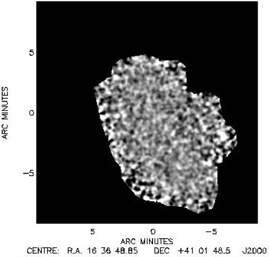
Figure 5: A pure noise image of the ELAIS N2 region, created from the real data by corrupting the astrometry of the individual jiggle maps to produce a ‘scrambled’ map. This image includes the jiggle maps taken up to and including 16th August 2000. There are no source detections at $>3.50\sigma$.

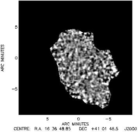
Figure 6: Fully-simulated ELAIS N2 SCUBA 850 ${\rm\mu m}$ map, using the adopted counts model given in Section 5.2. The image noise was simulated using the scrambled map shown in Figure 5.

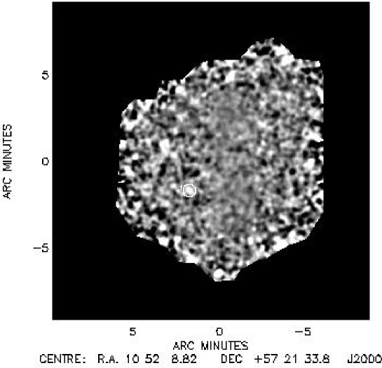
Figure 7: A pure noise image of the Lockman Hole East region, created from the real data by corrupting the astrometry of the individual jiggle maps to produce a ‘scrambled’ map. This image includes the jiggle maps taken up to and including 16th August 2000. There is one spurious source detection at $>3.50\sigma$ which is circled on the image.

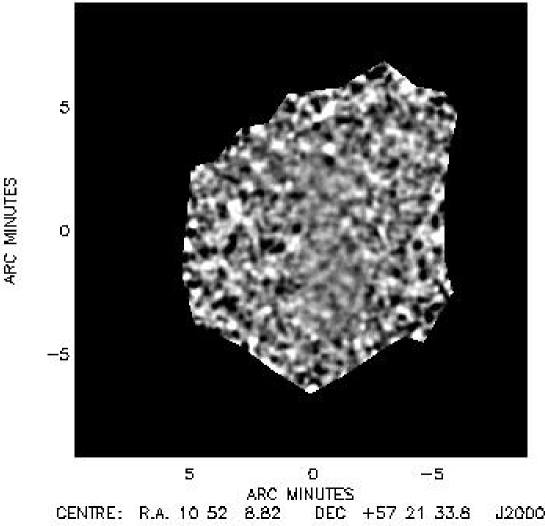
Figure 8: Fully-simulated Lockman Hole East SCUBA 850 ${\rm\mu m}$ map, using the adopted counts model given in Section 5.2. The image noise was simulated using the scrambled map shown in Figure 7.

A normalised beam map was used as a source template. At 0.5 mJy flux intervals, from 5 to 15 mJy, individual sources were added into the unconvolved zero-footprint signal maps. This was done one fake source at a time, so as not to enhance significantly any existing real confusion noise within the image. The source-extraction algorithm was then re-run. This exercise was repeated for 100 different randomly-selected positions on each image, at each flux level, so that source reclamation could be monitored as a function of input flux and position/noise-level within the maps. Source reclamation was deemed to have been successful if the source-extraction algorithm returned a source with signal-to-noise $>3.50$ within less than half a beam width of the input position. When analysing the output data, $\simeq 10\%$ of the input sources were found to lie within half a beam width of another peak $>5$ mJy already present in the image. Any such source was excluded from statistical analyses of positional error, completeness and error in reclaimed flux density, since the proportion of blends produced by two sources, both with comparably bright fluxes in the region of 8 mJy, should be negligible within our sample.

Figs 1 to 4 show the dependences of mean positional error, percentage of sources returned, systematic offset in returned flux density, and predicted output against input flux density, for both regions of uniform and non-uniform noise. The error bars show the standard error on the mean. The solid lines in Fig 1, and solid curves in Figs 2 and 3, are best-fit models to the plotted data points. From Fig 3, we see that the effect of noise and confusion is to produce systematic ‘flux boosting’, the retrieved flux density always being greater than the input value. The solid curves in Fig 4 show the predicted output versus input flux density based on the fitted flux-density boosting models of Fig 3. We find that there is a strong correlation with input flux density for each of these quantities, the scatter being somewhat larger in the areas of non-uniform noise lying towards the edge, as would be expected. The positional error and flux-density boosting factors decrease with increasing input flux density, whilst the percentage of sources returned at $>3.50\sigma$ increases. The effect of additional noise in the non-uniform regions considerably increases the uncertainty in positional error, as well as the mean flux-density boosting factor. It also serves to typically half the percentage of sources reclaimed. A summary of the results at 5, 8, 11 and 14 mJy is given in Table 1. The integral completeness down to each flux-density limit has been calculated by a counts-slope-weighted sum of the fraction of sources returned at each specific flux-density level, based on an adopted 850 ${\rm\mu m}$ source counts model consistent with the measured source counts, given in Section 5.2. As detailed in Table 1, the typical completeness at 8 mJy is $\simeq 80\%$ within the uniform noise regions of the images, with flux-density boosting factors of $\simeq 15\%$. By 11 mJy completeness has risen to $\simeq 90\%$, while flux-density boosting has dropped to $<10\%$.

	ELAIS N2	ELAIS N2	Lockman Hole E	Lockman Hole E	All	All
	Uniform noise	Full area	Uniform noise	Full area	Uniform noise	Full area
Area (sq. arcmin)	63	102	55	122	118	224
Sources $>8$ mJy in	16	28	12	18	28	46
Sources $>8$ mJy out	18	25	16	20	34	45
Real sources $>8$ mJy out	12	16	10	13	22	29
Confused sources $>8$ mJy	11	01	02	02	03	03
Real boosted sources	15	08	04	05	09	13
$>5$ mJy in, $>8$ mJy out
% completeness	$75.0\pm 21.7$	$\phantom{1}57.1\pm 14.3$	$83.3\pm 26.4$	$72.2\pm 20.0$	$78.6\pm 16.8$	$\phantom{1}63.0\pm 11.7$
% confused/random	$\phantom{0}5.6\pm\phantom{0}5.6$	$\phantom{10}4.0\pm\phantom{0}4.0$	$12.5\pm\phantom{0}8.8$	$10.0\pm\phantom{0}7.1$	$\phantom{0}8.8\pm\phantom{0}5.1$	$\phantom{10}6.7\pm\phantom{0}3.8$
% count correction factor	$88.9\pm 22.2$	$112.0\pm 21.2$	$75.0\pm 21.7$	$90.0\pm 21.2$	$82.4\pm 15.6$	$102.2\pm 15.1$

Table 2: Results of the completeness simulations at the $4.00\sigma$ significance level, in which each field was fully simulated 4 times using an adopted counts model consistent with the measured source counts. The sources were then retrieved by means of the maximum-likelihood estimator outlined in Section 4.

	ELAIS N2	ELAIS N2	Lockman Hole E	Lockman Hole E	All	All
	Uniform noise	Full area	Uniform noise	Full area	Uniform noise	Full area
Area (sq. arcmin)	63	102	55	122	118	224
Sources $>8$ mJy in	16	28	12	18	28	46
Sources $>8$ mJy out	23	32	19	24	42	56
Real sources $>8$ mJy out	13	17	11	14	24	31
Confused sources $>8$ mJy	04	05	04	05	08	10
Real boosted sources	06	10	04	05	10	15
$>5$ mJy in, $>8$ mJy out
% completeness	$81.3\pm 22.5$	$60.7\pm 14.7$	$91.7\pm 27.6$	$77.8\pm 20.8$	$85.7\pm 17.5$	$67.4\pm 12.1$
% confused/random	$17.4\pm\phantom{0}8.7$	$15.6\pm\phantom{0}7.0$	$21.1\pm 10.5$	$20.8\pm\phantom{0}9.3$	$19.0\pm\phantom{0}6.7$	$17.9\pm\phantom{0}5.6$
% count correction factor	$69.6\pm 17.4$	$87.5\pm 16.5$	$63.0\pm 18.2$	$75.0\pm 17.7$	$66.7\pm 12.6$	$82.1\pm 12.1$

Table 3: Results of the completeness simulations at the $3.50\sigma$ significance level, in which each field was fully simulated 4 times using an adopted counts model consistent with the measured source counts. The sources were then retrieved by means of the maximum-likelihood estimator outlined in Section 4.

	ELAIS N2	ELAIS N2	Lockman Hole E	Lockman Hole E	All	All
	Uniform noise	Full area	Uniform noise	Full area	Uniform noise	Full area
Area (sq. arcmin)	63	102	55	122	118	224
Sources $>8$ mJy in	16	28	12	18	28	46
Sources $>8$ mJy out	26	50	31	49	57	99
Real sources $>8$ mJy out	13	19	11	14	24	33
Confused sources $>8$ mJy	07	20	16	28	23	48
Real boosted sources	06	11	04	07	10	18
$>5$ mJy in, $>8$ mJy out
% completeness	$81.3\pm 22.5$	$67.9\pm 15.6$	$91.7\pm 27.6$	$77.8\pm 20.8$	$85.7\pm 17.5$	$71.7\pm 12.5$
% confused/random	$26.9\pm 10.2$	$40.0\pm\phantom{0}8.9$	$51.6\pm 12.9$	$57.1\pm 10.8$	$40.4\pm\phantom{0}8.4$	$48.5\pm\phantom{0}7.0$
% count correction factor	$61.5\pm 15.4$	$56.0\pm 10.6$	$38.7\pm 11.2$	$36.7\pm\phantom{0}8.7$	$49.1\pm\phantom{0}9.3$	$46.5\pm\phantom{0}6.9$

Table 4: Results of the completeness simulations at the $3.00\sigma$ significance level, in which each field was fully simulated 4 times using an adopted counts model consistent with the measured source counts. The sources were then retrieved by means of the maximum-likelihood estimator outlined in Section 4.

5.2 Completely simulated maps

Adopting an 850 ${\rm\mu m}$ source counts model consistent with the measured point source counts, and which does not over-predict the FIR background, we have created fully-simulated versions of our two survey fields. In order to produce a realistic model of the background counts, the number of sources expected at 0.1 mJy intervals was Gaussian randomised and then the appropriate sources were planted into the simulated data sets at random positions. The whole image was then convolved with the beam. At all flux-density levels the sources were assumed to be un-clustered (although see Section 9.4 and Almaini et al. 2002).

We then constructed a pure noise image for each of our two fields by scrambling the astrometry of the individual SCUBA observations used to produce the maps. These may be seen in Figs 5 and 7. After creating the scrambled noise maps we first ran the source-extraction algorithm on these to assess the frequency with which spurious sources would artificially appear on the basis of random statistics. The noise images yielded only a single artificial source at $>3.50\sigma$, and a total of 12 spurious sources at $>3.00\sigma$, which is not unexpected given the $\simeq 1200$ beams across the areas of these maps. Adding the simulated background counts to the scrambled maps produces the final simulated images. The source-extraction algorithm was applied as previously.

Four realisations of the sky in each field were generated for the source counts model

$$\frac{dN(>S)}{dS}=\frac{N_{0}}{S_{0}}\left(\left(\frac{S}{S_{0}}\right)^{\alpha}+\left(\frac{S}{S_{0}}\right)^{\beta}\right)^{-1}$$ (1)

where $N_{0}=1.1\times 10^{4}\mathrm{deg^{-2}mJy^{-1}}$ , $S_{0}=1.79$ mJy, $\alpha~{}=~{}0.0$, and $\beta~{}=~{}3.13$. Examples of the simulated ELAIS N2 and Lockman Hole East maps for our adopted counts model may be seen in Figs 6 and 8.

Tables 2 to 4 summarise the results at 4.00, 3.50 and 3.00$\sigma$ respectively for the simulated fields at 8 mJy. In these tables and the discussion that follows, we have adopted the practical criterion that any source retrieved at the 8 mJy level which ultimately could not be identified with a single source brighter than 5 mJy (and therefore could not be confirmed through interferometric follow-up for example), should be regarded as spurious or the result of confusion. In the uniform noise regions, contamination from spurious sources or confused sources $<5$ mJy is $\simeq 40\%$ at S/N $>3.00$, dropping to $\simeq 20\%$ at S/N $>3.50$ and $<10\%$ at S/N $>4.00$. The completeness at a measured flux density of 8 mJy is $\simeq 85\%$ within the regions of uniform noise, consistent with the completeness determined from the simulations using the real survey data. We also find that although the real source counts (ie. total number of sources out minus the number of spurious sources) at $>3.50\sigma$ agree well with the number planted into the simulations at 8 mJy, this is partly by chance; the number of sources boosted from a lower flux-density level, between 5 and 8 mJy, is approximately the same as the number of real sources $>8$ mJy which are not retrieved by the source-extraction algorithm. By lowering our signal-to-noise threshold from 3.50 to 3.00, there is very little improvement (if any) in completeness, however the proportion of spurious sources detected is much more serious. These results provide a clear motivation for setting a signal-to-noise threshold of $>3.50$ when determining the source number counts as opposed to the $>3.00\sigma$ level applied in some other surveys. Our results are consistent with those of Hughes & Gaztañaga (2000), who have simulated sub-millimetre galaxy surveys for a range of wavelengths, spatial resolutions and flux densities.

Figure 9: The 850 ${\rm\mu m}$ image of the ELAIS N2 field, smoothed with a beam-size Gaussian (14.5 arcsec FWHM). The numbered circles highlight those sources found at a significance of $>3.50$, the labels corresponding to the numbers in Table 5.

Source	RA	DEC	$S_{850}\phantom{00}$	S/N	Noise	$S_{450}$ or $3\sigma$	S/N	$S_{450}$ of any	S/N	Distance
	(J2000)	(J2000)	/mJy00	850 ${\rm\mu m}$	Region	up. lim. at	450 ${\rm\mu m}$	$>3\sigma$ source	450 ${\rm\mu m}$	from
						850 ${\rm\mu m}$ pos.	at	$<8.0^{\prime\prime}$ from	at	850 ${\rm\mu m}$
						/mJy	850 ${\rm\mu m}$	850 ${\rm\mu m}$ pos	450 ${\rm\mu m}$	peak
							pos	/mJy	pos	/arcsec
01	16:37:04.3	41:05:30	$11.2\pm 1.6$	8.59	uniform	$\phantom{<}30\pm 10$	3.82	$32\pm 10$	4.08	2.0
02	16:36:58.7	41:05:24	$10.7\pm 2.0$	6.27	uniform	$\phantom{<}30\pm 9$	4.10	$30\pm\phantom{1}9$	4.16	2.0
03	16:36:58.2	41:04:42	$8.5\pm 1.6$	5.86	uniform	$<26$
04	16:36:50.0	40:57:33	$8.2\pm 1.7$	5.18	uniform	$<34$
05	16:36:35.6	40:55:58	$8.5\pm 2.2$	4.16	uniform	$<35$
06	16:37:04.2	40:55:45	$9.2\pm 2.4$	4.13	uniform	$<91$		$73\pm 28$	3.09	4.5
07	16:36:39.4	40:56:38	$9.0\pm 2.4$	4.07	uniform	$<39$
08	16:36:58.8	40:57:33	$5.1\pm 1.4$	3.82	uniform	$<43$
09	16:36:22.4	40:57:05	$9.0\pm 2.5$	3.76	non-uni	$<88$
10	16:36:48.8	40:55:54	$5.4\pm 1.5$	3.69	uniform	$<47$		$39\pm 15$	3.18	5.7
11	16:36:44.5	40:58:38	$7.1\pm 2.0$	3.67	uniform	$<48$
12	16:37:02.5	41:01:23	$5.5\pm 1.6$	3.65	uniform	$<42$
13	16:36:31.2	40:55:47	$6.3\pm 1.9$	3.56	uniform	$<68$
14	16:36:19.7	40:56:23	$11.2\pm 3.3$	3.55	non-uni	$<43$
15	16:37:10.2	41:00:17	$5.0\pm 1.5$	3.52	uniform	$<18$
16	16:36:52.3	41:05:52	$12.9\pm 3.9$	3.51	non-uni	$<18$
17	16:36:51.4	41:05:06	$5.7\pm 1.7$	3.50	uniform	$<23$
18	16:36:11.4	40:59:26	$20.8\pm 6.2$	3.49	non-uni	$<138$
19	16:36:35.9	41:01:38	$9.4\pm 2.8$	3.49	uniform	$<76$
20	16:36:49.4	41:04:17	$6.6\pm 2.0$	3.48	uniform	$\phantom{<}22\pm 8$	3.32	$20\pm\phantom{1}8$	3.05	3.2
21	16:37:10.5	41:00:49	$4.9\pm 1.5$	3.47	uniform	$<23$
22	16:36:27.9	40:54:04	$13.4\pm 4.1$	3.46	non-uni	$<102$
23	16:37:19.5	41:01:38	$12.4\pm 3.8$	3.45	non-uni	$<40$
24	16:36:26.9	41:02:23	$10.4\pm 3.2$	3.43	non-uni	$<44$
25	16:36:18.3	40:59:12	$12.1\pm 3.8$	3.37	non-uni	$<57$
26	16:36:32.0	41:00:05	$9.7\pm 3.1$	3.26	uniform	$<27$
27	16:36:48.3	41:03:52	$6.6\pm 2.1$	3.25	uniform	$<21$
28	16:36:47.2	41:04:48	$6.3\pm 2.0$	3.24	uniform	$<22$
29	16:36:24.1	40:59:35	$9.9\pm 3.3$	3.14	uniform	$<70$
30	16:37:07.5	41:02:37	$4.6\pm 1.5$	3.13	uniform	$<40$
31	16:36:28.1	41:01:41	$6.8\pm 2.3$	3.07	uniform	$<36$
32	16:36:39.8	41:00:34	$5.4\pm 1.8$	3.07	uniform	$<27$
33	16:36:50.5	40:58:54	$4.8\pm 1.6$	3.06	uniform	$<34$
34	16:36:27.0	40:58:15	$6.9\pm 2.3$	3.05	uniform	$<36$
35	16:36:44.8	40:56:51	$5.5\pm 1.9$	3.02	uniform	$<23$
36	16:36:52.9	41:02:52	$3.8\pm 1.3$	3.00	uniform	n/a

Table 5: Sources retrieved in the long-wavelength ELAIS N2 image above the $3.00\sigma$ significance level using the source-extraction algorithm outlined in Section 4. We used a peak-normalised calibrator beam-map as a source template, and constructed a basic model by centring a beam-map at the positions of all peaks $>3$ mJy as found in the 14.5^′′ FWHM Gaussian convolved maps. The heights of each of the positioned beam maps were allowed to vary simultaneously such that the final model satisfied a minimised $\chi^{2}$ fit. We suggest that follow-up observations be confined to those detections $>3.50\sigma$ given the serious problem of contamination by spurious sources at the $3.00\sigma$ level. Calibration errors of 9% and 20% at 850 ${\rm\mu m}$ and 450 ${\rm\mu m}$ respectively, are included in the error on the flux densities.

Figure 10: The 850 ${\rm\mu m}$ image of the Lockman Hole East field, smoothed with a beam-size Gaussian (14.5 arcsec FWHM). The numbered circles highlight those sources found at a significance of $>3.50$, the labels corresponding to the numbers in Table 6.

Source	RA	DEC	$S_{850}\phantom{00}$	S/N	Noise	$S_{450}$ or $3\sigma$	S/N	$S_{450}$ of any	S/N	Distance
	(J2000)	(J2000)	/mJy00	850 ${\rm\mu m}$	Region	up. lim. at	450 ${\rm\mu m}$	$>3\sigma$ source	450 ${\rm\mu m}$	from
						850 ${\rm\mu m}$ pos.	at	$<8.0^{\prime\prime}$ from	at	850 ${\rm\mu m}$
						/mJy	850 ${\rm\mu m}$	850 ${\rm\mu m}$ pos	450 ${\rm\mu m}$	peak
							pos	/mJy	pos	/arcsec
01	10:52:01.4	57:24:43	$10.5\pm 1.6$	8.10	deep	$<\phantom{1}43$		$45\pm 13$	4.64	5.0
02	10:52:38.2	57:24:36	$10.9\pm 2.4$	5.22	uniform	$<\phantom{1}41$
03	10:51:58.3	57:18:01	$7.7\pm 1.7$	5.06	deep	$<\phantom{1}54$		$39\pm 14$	3.38	3.2
04	10:52:04.1	57:25:28	$8.3\pm 1.8$	5.03	deep	$<\phantom{1}51$
05	10:51:59.3	57:17:18	$8.6\pm 2.0$	4.57	deep	$<\phantom{1}34$
06	10:52:30.6	57:22:12	$11.0\pm 2.6$	4.50	uniform	$<101$
07	10:51:51.5	57:26:35	$8.1\pm 1.9$	4.50	deep	$<\phantom{1}86$
08	10:52:00.0	57:24:21	$5.1\pm 1.3$	4.38	deep	$<\phantom{1}17$
09	10:52:22.7	57:19:32	$12.6\pm 3.2$	4.20	uniform	$<\phantom{1}47$
10	10:51:42.4	57:24:45	$12.2\pm 3.1$	4.18	uniform	$<124$
11	10:51:30.6	57:20:38	$13.5\pm 3.5$	4.09	non-uni	$<\phantom{1}90$		$65\pm 24$	3.32	6.0
12	10:52:07.7	57:19:07	$6.2\pm 1.6$	4.01	deep	$<\phantom{1}55$
13	10:51:33.6	57:26:41	$9.8\pm 2.8$	3.69	uniform	$<\phantom{1}90$
14	10:52:04.3	57:26:59	$9.5\pm 2.8$	3.61	uniform	$<274$
15	10:52:24.6	57:21:19	$11.7\pm 3.4$	3.60	uniform	$<\phantom{1}53$
16	10:52:27.1	57:25:16	$6.1\pm 1.8$	3.56	uniform	$<\phantom{1}39$
17	10:52:16.8	57:19:23	$9.2\pm 2.7$	3.55	uniform	$<\phantom{1}57$
18	10:51:55.7	57:23:12	$4.5\pm 1.3$	3.55	deep	$<\phantom{1}36$
19	10:52:29.7	57:26:19	$5.5\pm 1.6$	3.54	uniform	$<\phantom{1}39$
20	10:52:37.7	57:20:30	$10.3\pm 3.1$	3.51	non-uni	$<\phantom{1}73$
21	10:52:01.7	57:19:16	$4.5\pm 1.3$	3.50	deep	$<\phantom{1}35$
22	10:52:05.7	57:20:53	$4.7\pm 1.4$	3.49	deep	$<\phantom{1}52$
23	10:51:47.0	57:24:51	$7.4\pm 2.2$	3.48	uniform	$<\phantom{1}60$
24	10:51:42.9	57:24:12	$11.4\pm 3.4$	3.47	uniform	$<\phantom{1}63$
25	10:52:36.0	57:18:20	$12.7\pm 3.8$	3.46	non-uni	$<137$
26	10:52:27.3	57:19:06	$8.3\pm 2.6$	3.39	uniform	$<\phantom{1}59$
27	10:51:53.8	57:18:47	$5.5\pm 1.7$	3.38	deep	$<\phantom{1}33$
28	10:52:34.6	57:20:02	$10.2\pm 3.2$	3.31	uniform	$<\phantom{1}74$
29	10:52:16.4	57:25:07	$6.7\pm 2.1$	3.30	uniform	$<\phantom{1}28$
30	10:52:42.2	57:18:28	$11.2\pm 3.6$	3.25	non-uni	$<\phantom{1}92$
31	10:52:03.9	57:20:07	$4.0\pm 1.3$	3.24	deep	$<\phantom{1}22$
32	10:52:00.0	57:20:39	$4.3\pm 1.4$	3.22	deep	$<\phantom{1}24$
33	10:51:33.8	57:19:29	$8.1\pm 2.6$	3.20	uniform	$<\phantom{1}75$
34	10:52:09.9	57:20:40	$8.5\pm 2.8$	3.16	uniform	$<\phantom{1}77$
35	10:51:57.6	57:26:03	$6.7\pm 2.3$	3.02	uniform	$<\phantom{1}91$
36	10:52:03.5	57:16:54	$8.0\pm 2.8$	3.00	uniform	$<\phantom{1}29$

Table 6: Sources retrieved in the Lockman Hole East field above the $3.00\sigma$ significance level using the source extraction algorithm outlined in Section 4.We used a peak-normalised calibrator beam-map as a source template, and constructed a basic model by centring a beam-map at the positions of all peaks $>3$ mJy as found in the 14.5” FWHM Gaussian convolved maps. The heights of each of the positioned beam maps were allowed to vary simultaneously such that the final model satisfied a minimised $\chi^{2}$ fit. We suggest that follow-up observations are confined to those detections $>3.50\sigma$ given the serious problem of contamination by spurious sources at the $3.00\sigma$ level.Calibration errors of 9% and 20% at 850 ${\rm\mu m}$ and 450 ${\rm\mu m}$ respectively, are included in the error on the flux densities.

6 Sources

Sources down to a significance level of $>3.00\sigma$ at 850 ${\rm\mu m}$ are listed in Table 5 for ELAIS N2 and Table 6 for the Lockman Hole East, ranked in order of formal significance as determined from our maximum-likelihood extraction technique. The top section of each table, containing 7 and 12 sources in ELAIS N2 and Lockman Hole East respectively, is confined to sources for which the S/N $>4.00$, and the middle section to sources for which S/N $>3.50$. Since our simulations indicate that 70-80% of these sources are expected to be real individual sources with flux densities within $\simeq 25\%$ of the extracted flux density, we recommend that follow-up observations are confined to these abbreviated S/N $>3.50$ source lists. The 850 ${\rm\mu m}$ flux densities in column 4 are the best-fit scaling factors determined by our extraction algorithm, with the quoted errors also incorporating the 9% calibration error.

Figs 9 and 10 show the beam-sized Gaussian convolved survey maps at 850 ${\rm\mu m}$ for ELAIS N2 and the Lockman Hole East respectively, with the sources $>3.50\sigma$ circled and numbered. We have also applied our maximum-likelihood estimator to the 450 ${\rm\mu m}$ data (Fox et al. 2002), centring normalised 450 ${\rm\mu m}$ beam maps at the same positions as in the 850 ${\rm\mu m}$ images. Column 7 gives the 450 ${\rm\mu m}$ flux densities if there is a detection in the short-wavelength data with S/N $>3.00\sigma$, or, more commonly, a $3\sigma$-upper-limit. We also carried out a search for peaks in the short-wavelength data lying within a search radius of 8 arcsec from the 850 ${\rm\mu m}$ source peaks (the combined result of adding in quadrature the 1/2 beam-width positional uncertainties of the long- and short-wavelength data) and again employed our source-extraction algorithm. The flux densities of any detections with S/N better than $3.00\sigma$ are given in column 9, with their significances and positional offset from the long-wavelength position in columns 10 and 11. The errors quoted on the 450 ${\rm\mu m}$ flux densities also include the 20% calibration error.

Given that the FWHM of the JCMT beam at 850 ${\rm\mu m}$ is 14.5 arcsec, the source positions are only likely to be accurate to within $\simeq 3-4$ arcsec. Consistent with this, our simulations suggest that an 8 mJy source, detected at $>3.50\sigma$, should have accurate astrometry to $\sim 3.5$ arcsec in uniform noise regions and $\sim 4$ arcsec in the non-uniform noise areas, the positional uncertainty decreasing with increasing flux. However, these simulations do not account for the elevation drive pointing glitch mentioned in Section 3.2, and so it is possible that the astrometric accuracy of a source affected by this problem could be somewhat worse than this.

Analysis of our fully-simulated survey areas suggests that of the 19 sources with S/N $>4.00$, only one is likely to be spurious. At the $3.50\sigma$ threshold we have 38 sources, of which $\simeq 7$ may be spurious. The situation is markedly worse at $3.00\sigma$, where $\simeq 30$ of the supposedly-significant peaks may in fact be due to noise or confusion of low flux-density sources.

In the short-wavelength data, we can find only 3 detections at $>4.00\sigma$ within an 8 arcsec radius of the 850 ${\rm\mu m}$ positions. These 450 ${\rm\mu m}$ detections appear to be associated with the most significant Lockman Hole East 850 ${\rm\mu m}$ source and the two most significant ELAIS N2 850 ${\rm\mu m}$ sources. There are additionally another five 450 ${\rm\mu m}$ detections at better than $3.00\sigma$, of which all but one is associated with a $>3.50\sigma$ 850 ${\rm\mu m}$ source. We must be cautious when considering the credibility of the lower significance ($>3.00\sigma$) 450 ${\rm\mu m}$ detections. The atmospheric opacity at 450 ${\rm\mu m}$ is much more sensitive to changes in the amount of water vapour present than at 850 ${\rm\mu m}$, and so the resulting short-wavelength maps are noisier than their long-wavelength counterparts. Furthermore, the smaller beam-size (7.5 arcsec FWHM at 450 ${\rm\mu m}$ as opposed to 14.5 arcsec FWHM at 850 ${\rm\mu m}$) means that the short-wavelength maps will contain a greater number of spurious detections. For S/N $>3.00$ we would expect 53 spurious sources across the full 260 $\mathrm{arcmin^{2}}$ of short-wavelength data ( and 14 spurious detections in the long-wavelength data) based on Gaussian statistics alone.

A detailed discussion of individual sources may be found in paper II of the SCUBA 8 mJy survey (Fox et al., 2002), along with a multiwavelength analysis considering possible identifications and SED-based redshift constraints. The 450 ${\rm\mu m}$ images of the survey fields are also presented by Fox et al. (2002).

Flux density	Number	N($>\mathrm{S}$)	Number after	Number after	N($>\mathrm{S}$)
/mJy	observed	observed	flux boost	flux boost &	corrected
			correction	completeness
				correction
15.0	3	31	0	0.00	32.9
15.5	4	28	1	3.59	32.9
16.0	2	24	0	0.00	29.3
16.5	1	22	3	6.55	29.3
17.0	1	21	3	5.66	22.7
17.5	1	20	0	0.00	17.1
18.0	2	19	3	4.64	17.1
18.5	4	17	1	1.44	12.4
19.0	3	13	1	1.36	11.0
19.5	1	19	0	0.00	19.6
10.0	1	19	3	3.75	19.6
10.5	2	18	2	2.42	15.8
11.0	3	16	0	0.00	13.4
11.5	1	13	1	1.15	13.4
12.0	1	12	1	1.13	12.2
12.5	1	11	1	1.11	11.1
13.0	0	10	0	0.00	10.0

Table 7: A breakdown of the raw and corrected source counts at each 0.5 mJy interval bin for the sources with S/N $>3.50$ from both survey maps, excluding those uncovered in the non-uniform noise regions. Column 1 gives the flux density, and columns 2 and 3 the raw number counts in the 0.5 mJy wide bin and cumulative to that flux-density level. Column 4 gives the number in each bin once flux-density boosting has been accounted for using the fitted curve in Fig 4(a), and similarly column 5 gives the number in each bin once completeness has also been taken into account using the fitted curve in Fig 2(a). Column 6 gives the cumulative corrected counts down to each flux-density level.

Flux density	Raw 850 ${\rm\mu m}$ source counts	Corrected 850 ${\rm\mu m}$ source counts
/mJy	$N(>S)\mathrm{deg^{-2}}$	$N(>S)\mathrm{deg^{-2}}$
15	$580\pm 100$	$620^{+110}_{-190}$
16	$450\pm 90$0	$550^{+100}_{-170}$
17	$400\pm 90$0	$430^{+90}_{-120}$
18	$360\pm 80$0	$320^{+80}_{-100}$
19	$250\pm 70$0	$200^{+60}_{-70\phantom{0}}$
10	$170\pm 60$0	$180^{+60}_{-60\phantom{0}}$
11	$110\pm 50$0	1$60^{+30}_{-30\phantom{0}}$
12	1$40\pm 30$0	1$40^{+30}_{-30\phantom{0}}$

Table 8: The 850 ${\rm\mu m}$ source counts per square degree based on sources with S/N $>3.50$ in both survey maps, and excluding those detected in the non-uniform noise regions. Column 1 gives the flux density and column 2 the cumulative raw counts per square degree with the Poisson error. Column 3 gives the cumulative corrected counts per square degree, the upper error corresponding to the Poisson error, and the lower error accounting for both the Poisson error and the presence of spurious sources based on the simulation data.

7 Number counts

In order to obtain the best estimate of the number counts at 850 ${\rm\mu m}$, we must account for the effects of flux-density boosting, incompleteness and contamination from spurious sources. Using the results of our simulations carried out on the real survey data, the observed flux densities of the $>3.50\sigma$ sources were corrected statistically using the output flux density versus input flux density plots shown in Fig 4, for the appropriate image noise region. The number of boost-corrected sources in bins 0.5 mJy wide, centred on 5.0, 5.5, 6.0 mJy and so on up to 15 mJy, were then amended for completeness using the best fit results of the real-data simulations shown in Fig 2. The integrated source counts were obtained by summing the number of sources in the bins down to the required threshold flux. Since the scatter in the simulation results is substantially higher in the non-uniform noise regions (reflected by reduced $\chi^{2}$ values of the plotted best-fit curves being a factor of $\sim 5$ higher in the edge regions), we have based our estimation of the 850 ${\rm\mu m}$ source counts purely on the sources detected in the areas of uniform noise, covering an area of 190 $\mathrm{arcmin^{2}}$. In practice this means that 5/38 of the sources above the $3.50\sigma$ significance threshold have been excluded. This process is summarised in Table 7, with the raw and amended counts per square degree shown in Table 8, along with Poisson errors.

The applied correction factors have been determined from simulations carried out on the real images and so are independent of source-count models. We cannot, however, attempt to correct for the presence of random detections without making some assumptions about the background counts. Consequently, the estimated number of spurious sources is included in the lower error bars combined in quadrature with the Poisson error, rather than being applied directly to the actual tabulated source-count values.

Fig 11 shows our corrected source counts, at 1 mJy intervals, from 5 to 12 mJy, along with data points from other SCUBA surveys (Barger, Cowie & Sanders 1999, Blain et al. 1999, Eales et al. 2000, Hughes et al 1998, and Smail et al. 1997). The upper solid and dashed lines in Fig 11 are source-count models, derived by interpolating the 60 $\rm\mu m$ luminosity function (Saunders et al., 1990) to 850 $\rm\mu m$, with an assumed dust temperature of 40K and dust emissivity index $\beta=1.2$ (consistent with measurements of local ULIRGs such as Arp220 eg. Dunne et al. 2000), and assuming pure luminosity evolution of the form $L(z)=L(0)(1+z)^{3}$ to $z=2.0$ (beyond which the luminosity function is simply frozen). The solid line assumes an Einstein-de Sitter cosmology, whereas the dashed line assumes the cosmology $\Omega_{M}=0.3$ and $\Omega_{\Lambda}=0.7$ (both adopting $H_{0}=67$ ${\rm kms^{-1}Mpc^{-1}}$). The lower solid and dashed lines represent the same interpolated 60 $\rm\mu m$ luminosity function with no luminosity evolution included, again for cosmologies $\Omega_{M}=1.0$, $\Omega_{\Lambda}=0.0$, and $\Omega_{M}=0.3$, $\Omega_{\Lambda}=0.7$ respectively. The dotted line shows the adopted source counts model, which was assumed when creating the fully-simulated images. The dot-dash and dot-dot-dash lines represent a more physical form of luminosity evolution (Jameson 2000, Smail et al. 2001), which is compatible with models of cosmic chemical evolution and includes a peak in the evolution function:

$$L(z)=L(0)(1+z)^{3/2}\mathrm{sech^{2}[b~{}ln(1+\mathit{z}\mathrm{)}-c]cosh^{2}c}$$ (2)

where $\mathrm{b=2.2\pm 0.1}$ and $\mathrm{c=1.84\pm 0.1}$. The dot-dash line assumes a cosmology $\Omega_{M}=1.0$, $\Omega_{\Lambda}=0.0$, and the dot-dot-dash line $\Omega_{M}=0.3$, $\Omega_{\Lambda}=0.7$. A dust emissivity index of $\beta=1.2$ and a dust temperature of 37K were also assumed (Smail et al. 2001).

8 2-point correlation functions

In order to obtain a first measure of the clustering properties of each of our two fields, we have used our $>3.50\sigma$ sources to calculate 2-point angular correlation functions for both ELAIS N2 and the Lockman Hole East. We created a catalogue for each survey area, containing $\sim 40000$ fake sources placed according to a Poisson distribution within the boundaries of the real data. Although the positions were generated at random, we used our uncorrelated noise maps to weight the number density of sources across the image, since we would expect to uncover a larger density of sources above a specified signal-to-noise threshold in areas of lower noise. In practise, we divided the full image into a series of sub-images, 20 arcsec by 20 arcsec in size, and calculated the mean noise level in each of these grid sections. For sources brighter than $\simeq 5$ mJy, the number of sources expected above a constant signal-to-noise threshold will increase approximately as $N(>S)\propto S^{-1.5}$, and consequently we would expect the relative number of sources in each sub-image to scale as $\langle\mathrm{noise}\rangle^{-1.5}$.

The angular correlation function $w(\theta)$ describes the excess probability of finding a source at an angular separation $\theta$ from a source selected at random, over a random distribution. There are a variety of possible estimators for $w(\theta)$ as a function of pair-count ratios. Here we have used:

$$1+w(\theta)=\frac{2m}{(n-1)}\frac{\langle DD\rangle}{\langle DR\rangle}$$ (3)

where there are $n$ and $m$ objects in the real and mock catalogues respectively, $DD$ is the number of distinct data pairs in the real image within a bin covering a specified range of $\theta$, and $DR$ is the number of cross-pairs between the real and fake catalogues within the same range of $\theta$.

The angular correlation functions may be seen with Poisson errors in Figs 12 and 13, where a bin size of twice the beam (29.0 arceconds) has been used.

Figure 11: Cumulative 850 $\rm\mu m$ source counts. The solid diamonds show the new results from the ‘SCUBA 8 mJy Survey’ derived in this paper. The upper solid and dashed curves are predicted number counts, based on the 60 $\rm\mu m$ luminosity function of Saunders et al. (1990), assuming a dust temperature of 40 K, a dust emissivity index of $\beta=1.2$, and pure luminosity evolution of the form $L(z)=L(0)(1+z)^{3}$ out to $z=2$ (beyond which the luminosity function is simply frozen), for cosmologies ($\Omega_{M}=1.0$,$\Omega_{\Lambda}=0.0$) and ($\Omega_{M}=0.3$,$\Omega_{\Lambda}=0.7$) respectively. The lower solid and dashed curves show the number counts predicted by the same models if no luminosity evolution is included. The dotted line shows the counts model assumed when creating simulated images. The dot-dash and dot-dot dash assume a more complicated, but arguably more realistic luminosity evolution of the form $L(z)=L(0)(1+z)^{3/2}\mathrm{sech^{2}[b~{}ln(1+\mathit{z}\mathrm{)}-c]cosh^{2}c}$ , for cosmologies ($\Omega_{M}=1.0$,$\Omega_{\Lambda}=0.0$) and ($\Omega_{M}=0.3$,$\Omega_{\Lambda}=0.7$) respectively, and assuming a dust temperature of 37K and dust emissivity index of $\beta=1.2$ (Jameson 2000, Smail et al. 2002).

9 Discussion

9.1 Comparative Source Counts and Models

Although our survey was undertaken with the aim of constraining the brighter end of the 850 $\rm\mu m$ number counts, we have in fact achieved the most accurate determination to date of the sub-mm source counts down to $S_{850}\simeq 5$ mJy. From Fig 11 we see that at 5 mJy there is good agreement between our counts $620^{+110}_{-190}\mathrm{deg^{-2}}$ and the values of Eales et al. (2000) $500\pm 200\mathrm{deg^{-2}}$, and Barger, Cowie & Sanders (1999) $610^{+240}_{-190}\mathrm{deg^{-2}}$, to well within the quoted errors. However, at larger flux densities, the number of sources per square degree in both the Eales and Barger survey areas is somewhat lower than our counts. For example at 6 mJy the number count of Eales et al. is a factor of $\sim 3$ lower than our value, and that of Barger, Cowie & Sanders (1999) is lower by a factor of $\sim 2.5$. The most likely explanation for this discrepancy is that it is due to small number statistics rather than a real steepening of the source counts at $>6$ mJy. We would in fact expect this to be the case if SCUBA sources were generally clustered on scales of a few arcmin (as indicated by our two-point autocorrelation functions, albeit with large errors, shown in Section 8 and discussed in Section 9.4). The “SCUBA 8 mJy Survey” covers 260 $\mathrm{arcmin^{2}}$ of sky, 5 times the area of the ‘Canada UK Deep Sub-millimetre Survey (CUDSS) 14h Field’ of Eales et al., and $\sim 2.5$ times the area of Barger et al., making us less susceptible to arcmin-scale clustering and thus leaving us much better able to constrain the number counts at brighter flux densities. At 8 mJy, Blain et al. (1999) suggest a rather higher count of $800\pm 600\mathrm{deg^{-2}}$ than our value of $320^{+80}_{-100}\mathrm{deg^{-2}}$, however the large error on the Blain et al. number count renders their result almost meaningless. At flux densities $>10$ mJy our survey also inevitably becomes limited by the lower surface density of brighter sources. In a similar manner to the source counts of Eales et al. and Barger et al. beyond 6 mJy, our counts at 11 and 12 mJy suggest a steepening of the counts slope towards brighter fluxes. Borys et al. (2002) report a number count of $164^{+78}_{-59}\mathrm{deg^{-2}}$ at 12 mJy, suggesting that this is again a statistical rather than a real effect.

The source counts accumulated across all the sub-millimetre surveys (as shown in Fig 11) are consistent with a population of high-redshift ($z>1$), dusty, star-forming galaxies, analogous to the local ULIRGs, with dust temperatures $T_{d}\sim 40$K, emissivity $\beta\sim 1.2$, and pure luminosity evolution of the form $(1+z)^{3}$ out to a redshift $z=2$ (and simply frozen beyond). We also find that our source counts are in very good agreement with the more physical form of luminosity evolution of Jameson (2000) and Smail et al. (2002), assuming a dust temperature of 37 K, particularly for the cosmology $\Omega_{M}=0.3$, $\Omega_{\Lambda}=0.7$. The lower solid and dashed lines show the predicted source counts using the same luminosity function but without any luminosity evolution. Such a model is inconsistent with the measured number counts by $2-3$ orders of magnitude, which simply serves to re-emphasise the extent of the evolution in the starburst population uncovered by SCUBA.

9.2 Dust Masses and Star Formation Rates

The photometric redshift estimates of the 19 sources discussed in Fox et al. (2002) and Lutz et al. (2001) are all indicative of redshifts $z>1$, and in the vast majority of cases favour $z>2$. Even without knowing a precise redshift, this fact coupled with an almost uniform sensitivity to objects between redshifts $z=1$ and $z=8$, allows us to make an estimate of the dust-enshrouded SFRs and dust masses. Assuming a dust temperature of 40K and emissivity index $\beta=1.2$, we have interpolated the inferred 850 $\rm\mu m$ luminosity to 60 $\rm\mu m$ using an optically-thin greybody approximation. The far-infrared luminosity provides a measure of the current SFR of massive stars. In regions of intense star formation, dust is heated primarily by the embedded O and B stars which evolve rapidly and dispense their surrounding material on similarly short time-scales ($\sim 10^{7}$ yr, Wang 1991), hence the rate of dust production is proportional to the star-formation rate. We may calculate the SFR to within a factor of a few, by means of

$$\mathrm{SFR}=\epsilon 10^{-10}\mathrm{\frac{L_{60}}{L_{\odot}}M_{\odot}yr^{-1}}$$ (4)

The value of $\epsilon$ is uncertain to within a factor of $\sim 3$ (Scoville & Young 1983, Thronson & Telesco 1986, Rowan-Robinson et al. 1997, Rowan-Robinson 2000), the main sources of error arising from uncertainties in the initial mass function (IMF), the fraction of optical/UV light absorbed by the dust, and the time-scale of the burst. We have assumed a value of $\epsilon=2.1$ (Thronson & Telesco 1986), which incorporates a burst of O,B, and A type star-formation over $\sim 2\times 10^{6}$ yr, and assumes a Salpeter IMF. It was also assumed that all of the optical/UV radiation was absorbed and re-radiated thermally by the surrounding dust.

Figure 12: 2-point angular correlation function for the ELAIS N2 survey field. $w(\theta)=\frac{2m}{n-1}\frac{\langle DD\rangle}{\langle DR\rangle}-1$ where there are n and m real and fake $>3.50\sigma$ sources respectively, and $DD$ and $DR$ are the number of distinct data pairs and cross data-random pairs within 29 arcsec width bins as a function of angular separation $\theta$. The power-law line indicates the correlation function found by Daddi et al. (2000) for EROs with $R-K>5$ and $K<18.5$ as discussed in Sections 9.3 and 9.4.

Figure 13: 2-point angular correlation function for the Lockman Hole East survey field. $w(\theta)=\frac{2m}{n-1}\frac{\langle DD\rangle}{\langle DR\rangle}-1$ where there are n and m real and fake $>3.50\sigma$ sources respectively, and $DD$ and $DR$ are the number of distinct data pairs and cross data-random pairs within 29 arcsec width bins as a function of angular separation $\theta$. The power-law line indicates the correlation function found by Daddi et al. (2000) for EROs with $R-K>5$ and $K<18.5$ as discussed in Sections 9.3 and 9.4. Note that the vertical dashed line demonstrates the cut-off at which there are no more source pairings in the real data.

In calculating the mass of dust present in each source, we assumed the sub-millimetre continuum to be the result of optically-thin thermal emission from the heated dust grains, with no additional contribution from bremsstrahlung or synchrotron radiation. We may then determine the dust mass $M_{d}$ by means of the relation

$$M_{d}=\frac{1}{1+z}\frac{S_{obs}D_{L}^{2}}{k_{d}^{\mathrm{rest}}B(\nu^{\mathrm{rest}},T_{d})}$$ (5)

where $z$ is the redshift of the source, $S_{obs}$ is the observed flux density, $D_{L}$ is the luminosity distance, $k_{d}^{\mathrm{rest}}$ is the rest-frequency mass absorption coefficient, and $B(\nu^{\mathrm{rest}},T_{d})$ is the rest-frequency value of the Planck function from dust grains radiating at temperature $T_{d}$. The main uncertainty in determining the dust mass $M_{d}$ is the uncertainty in the rest-frequency mass absorption coefficient $k_{d}^{\mathrm{rest}}$. We have adopted the same approach as Hughes, Dunlop & Rawlings (1997), using their average value of $k_{d}$(800 $\rm\mu m$)$=0.15\pm 0.09$ ${\rm m^{2}kg^{-1}}$, and interpolating to shorter wavelengths by assuming $k_{d}~{}\propto~{}\lambda^{-1.5}$. A different choice of $k_{d}$(800 $\rm\mu m$) would be expected to change the dust mass estimates by a factor of up to 2.

The results are outlined in Tables 9 and 10, the un-bracketted quantities assuming an Einstein-de Sitter cosmology, and the values enclosed in brackets adopting $\Omega_{M}=0.3$, $\Omega_{\Lambda}=0.7$. SFRs range from several hundred to several thousand solar masses per year (exceeding even that of the extreme local starburst Arp220), the star-forming activity being heavily obscured by $10^{8}-10^{9}~{}{\rm M_{\odot}}$ of dust. In fact, for $\Omega_{M}=0.3$, $\Omega_{\Lambda}=0.7$ and $H_{0}=67$ ${\rm kms^{-1}Mpc^{-1}}$ it can be seen that an 850 $\rm\mu m$ flux density of 8 mJy corresponds closely to a star-formation rate of $1000~{}{\rm M_{\odot}yr^{-1}}$.

The 19 sources brighter than 8 mJy, with $S/N>3.5$ and located in the uniform noise regions of the survey maps, account for $\simeq 10\%$ of the sub-millimetre background observed by COBE-FIRAS (Puget et al. 1996, Fixsen et al. 1998, Hauser et al. 1998). Table 11 shows the inferred star formation rate density for a variety of redshift bands, and for both of our adopted cosmologies. These bright SCUBA sources alone imply a high-redshift star formation rate density (SFRD) in the range $\simeq 0.01-0.07$ $\mathrm{M_{\odot}yr^{-1}Mpc^{-3}}$ , comparable to that observed in the optical/UV (Madau et al. 1996, Steidel et al. 1999). If we assume that the whole of the sub-millimtere background may be attributed to starlight reprocessed by dust, then this would imply a high-redshift SFRD in the range $\simeq 0.1-0.7$ $\mathrm{M_{\odot}yr^{-1}Mpc^{-3}}$, varying only by a factor of $2-3$ on the adopted redshift band for a given choice of cosmology. Our results agree very well with Barger, Cowie & Richards (2000) who considered the contribution to the SFRD of sources brighter than 6 mJy, and determined completeness corrected SFRDs $\simeq 0.1-0.4$ $\mathrm{M_{\odot}yr^{-1}Mpc^{-3}}$ in the redshift range $1<z<3$, and $\simeq 0.1-0.7$ $\mathrm{M_{\odot}yr^{-1}Mpc^{-3}}$ in the redshift range $3<z<6$. In contrast to the marked decline in the SFRD at $z>1$ originally implied by optical/UV observations (Madau et al. 1996), sub-millimetre surveys suggest that the SFRD is either steady or gently increasing to perhaps as far back as $z=5$. Current redshift constraints (Dunlop 2001a and references within) suggest that only $10-15\%$ of luminous ($>4$ mJy) sub-millimetre sources lie at $z<2$, and that the median redshift of this population is $z_{\mathrm{med}}\simeq 3$. A peak in the SFRD around this epoch would not be unexpected given the strong correlation between black-hole and spheroid mass found at low redshift (Kormendy & Gebhardt 2001) and the peak in optical emission from powerful quasars at $z\simeq 2.5$. However, improved redshift constraints are required to establish when (and indeed if) the comoving SFRD reached a maximum.

Source	RA	DEC	$S_{850}$00	S/N	Noise Region	$\mathrm{log_{10}L_{60}}$	SFR00	$\mathrm{log_{10}M_{dust}}$
	(J2000)	(J2000)	/mJy00	850 $\rm\mu m$	850 $\rm\mu m$	/$\mathrm{L_{\odot}}$	/$\mathrm{M_{\odot}yr^{-1}}$	/$\mathrm{M_{\odot}}$
01	16:37:04.3	41:05:30	$11.2\pm 1.6$	8.59	uniform	12.49 (12.83)	649 (1430)	8.62 (8.96)
02	16:36:58.7	41:05:24	$10.7\pm 2.0$	6.27	uniform	12.47 (12.82)	623 (1372)	8.60 (8.95)
03	16:36:58.2	41:04:42	$8.5\pm 1.6$	5.86	uniform	12.37 (12.71)	494 (1087)	8.50 (8.84)
04	16:36:50.1	40:57:33	$8.2\pm 1.7$	5.18	uniform	12.36 (12.70)	480 (1056)	8.49 (8.83)
05	16:36:35.6	40:55:58	$8.5\pm 2.2$	4.16	uniform	12.37 (12.71)	493 (1085)	8.50 (8.84)
06	16:37:04.2	40:55:45	$9.2\pm 2.4$	4.13	uniform	12.41 (12.75)	537 (1182)	8.54 (8.88)
07	16:36:39.4	40:56:38	$9.0\pm 2.4$	4.07	uniform	12.40 (12.74)	523 (1152)	8.53 (8.87)
08	16:36:58.8	40:57:33	$5.1\pm 1.4$	3.82	uniform	12.15 (12.49)	298 (1656)	8.28 (8.62)
09	16:36:22.4	40:57:05	$9.0\pm 2.5$	3.76	non-uniform	12.40 (12.74)	526 (1159)	8.53 (8.87)
10	16:36:48.8	40:55:54	$5.4\pm 1.5$	3.69	uniform	12.18 (12.52)	315 (1694)	8.31 (8.65)
11	16:36:44.5	40:58:38	$7.1\pm 2.0$	3.67	uniform	12.29 (12.63)	411 (1904)	8.42 (8.76)
12	16:37:02.5	41:01:23	$5.5\pm 1.6$	3.65	uniform	12.18 (12.52)	319 (1702)	8.31 (8.65)
13	16:36:31.2	40:55:47	$6.3\pm 1.9$	3.56	uniform	12.24 (12.58)	365 (1804)	8.37 (8.71)
14	16:36:19.7	40:56:23	$11.2\pm 3.3$	3.55	non-uniform	12.49 (12.83)	651 (1434)	8.62 (8.96)
15	16:37:10.2	41:00:17	$5.0\pm 1.5$	3.52	uniform	12.14 (12.48)	290 (1639)	8.27 (8.61)
16	16:36:52.3	41:05:52	$12.9\pm 3.9$	3.51	non-uniform	12.55 (12.90)	751 (1655)	8.68 (9.03)
17	16:36:51.4	41:05:06	$5.7\pm 1.7$	3.50	uniform	12.20 (12.54)	331 (1728)	8.33 (8.67)
18	16:36:11.4	40:59:26	$20.8\pm 6.2$	3.49	non-uniform	12.76 (13.10)	1212 (2669)	8.89 (9.23)
19	16:36:35.9	41:01:38	$9.4\pm 2.8$	3.49	uniform	12.42 (12.76)	550 (1211)	8.55 (8.89)
20	16:36:49.4	41:04:17	$6.6\pm 2.0$	3.48	uniform	12.26 (12.60)	383 (1844)	8.39 (8.73)
21	16:37:10.5	41:00:49	$4.9\pm 1.5$	3.47	uniform	12.13 (12.47)	283 (1624)	8.26 (8.60)
22	16:36:27.9	40:54:04	$13.4\pm 4.1$	3.46	non-uniform	12.57 (12.91)	780 (1718)	8.70 (9.04)
23	16:37:19.5	41:01:38	$12.4\pm 3.8$	3.45	non-uniform	12.54 (12.88)	721 (1587)	8.67 (9.01)
24	16:36:26.9	41:02:23	$10.4\pm 3.2$	3.43	non-uniform	12.46 (12.80)	607 (1336)	8.59 (8.93)
25	16:36:18.3	40:59:12	$12.1\pm 3.8$	3.37	non-uniform	12.52 (12.87)	703 (1548)	8.65 (9.00)
26	16:36:32.0	41:00:05	$9.7\pm 3.1$	3.26	uniform	12.43 (12.77)	567 (1248)	8.56 (8.90)
27	16:36:48.3	41:03:52	$6.6\pm 2.1$	3.25	uniform	12.26 (12.61)	386 (1851)	8.39 (8.74)
28	16:36:47.2	41:04:48	$6.3\pm 2.0$	3.24	uniform	12.24 (12.59)	367 (1809)	8.37 (8.72)
29	16:36:24.1	40:59:35	$9.9\pm 3.3$	3.14	uniform	12.44 (12.78)	573 (1263)	8.57 (8.91)
30	16:37:07.5	41:02:37	$4.6\pm 1.5$	3.13	uniform	12.11 (12.45)	268 (1590)	8.24 (8.58)
31	16:36:28.1	41:01:41	$6.8\pm 2.3$	3.07	uniform	12.27 (12.62)	393 (1866)	8.40 (8.75)
32	16:36:39.8	41:00:34	$5.4\pm 1.8$	3.07	uniform	12.18 (12.52)	315 (1694)	8.31 (8.65)
33	16:36:50.5	40:58:54	$4.8\pm 1.6$	3.06	uniform	12.12 (12.47)	280 (1616)	8.25 (8.60)
34	16:36:27.0	40:58:15	$6.9\pm 2.3$	3.05	uniform	12.28 (12.62)	400 (1881)	8.41 (8.75)
35	16:36:44.8	40:56:51	$5.5\pm 1.9$	3.02	uniform	12.18 (12.52)	318 (1700)	8.31 (8.65)
36	16:36:52.9	41:02:52	$3.8\pm 1.3$	3.00	uniform	12.02 (12.37)	222 (1489)	8.15 (8.50)

Table 9: Inferred FIR/60 $\rm\mu m$ luminosities, star-formation rates and dust masses for the sources in ELAIS N2. The un-bracketted numbers in columns 7, 8 and 9 assume an Einstein - de Sitter cosmology, whereas the numbers enclosed in brackets assume $\Omega_{M}=0.3$ and $\Omega_{\Lambda}=0.7$. A dust temperature of 40K, and emissivity index $\beta=1.2$ were assumed throughout, as was $H_{0}=67$ ${\rm kms^{-1}Mpc^{-1}}$.

Source	RA	DEC	$S_{850}$00	S/N	Noise Region	$\mathrm{log_{10}L_{60}}$	SFR00	$\mathrm{log_{10}M_{dust}}$
	(J2000)	(J2000)	/mJy00	850 $\rm\mu m$	850 $\rm\mu m$	/$\mathrm{L_{\odot}}$	/$\mathrm{M_{\odot}yr^{-1}}$	/$\mathrm{M_{\odot}}$
01	10:52:01.4	57:24:43	$10.5\pm 1.6$	8.10	deep strip	12.47 (12.81)	613 (1350)	8.60 (8.94)
02	10:52:38.2	57:24:36	$10.9\pm 2.4$	5.22	uniform	12.48 (12.82)	635 (1399)	8.61 (8.95)
03	10:51:58.3	57:18:01	$7.7\pm 1.7$	5.06	deep strip	12.33 (12.67)	448 (1987)	8.46 (8.80)
04	10:52:04.1	57:25:28	$8.3\pm 1.8$	5.03	deep strip	12.36 (12.71)	484 (1067)	8.49 (8.84)
05	10:51:59.3	57:17:18	$8.6\pm 2.0$	4.57	deep strip	12.38 (12.72)	500 (1100)	8.51 (8.85)
06	10:52:30.6	57:22:12	$11.0\pm 2.6$	4.50	uniform	12.48 (12.83)	638 (1405)	8.61 (8.96)
07	10:51:51.5	57:26:35	$8.1\pm 1.9$	4.50	deep strip	12.35 (12.70)	474 (1044)	8.48 (8.83)
08	10:52:00.0	57:24:21	$5.1\pm 1.3$	4.38	deep strip	12.15 (12.49)	295 (1649)	8.28 (8.62)
09	10:52:22.7	57:19:32	$12.6\pm 3.2$	4.20	uniform	12.54 (12.88)	736 (1620)	8.67 (9.02)
10	10:51:42.4	57:24:45	$12.2\pm 3.1$	4.18	uniform	12.53 (12.87)	712 (1567)	8.66 (9.00)
11	10:51:30.6	57:20:38	$13.5\pm 3.5$	4.09	non-uniform	12.57 (12.92)	786 (1731)	8.70 (9.05)
12	10:52:07.7	57:19:07	$6.2\pm 1.6$	4.01	deep strip	12.23 (12.58)	358 (1789)	8.36 (8.71)
13	10:51:33.6	57:26:41	$9.8\pm 2.8$	3.69	uniform	12.43 (12.78)	569 (1252)	8.56 (8.91)
14	10:52:04.3	57:26:59	$9.5\pm 2.8$	3.61	uniform	12.42 (12.76)	552 (1215)	8.55 (8.89)
15	10:52:24.6	57:21:19	$11.7\pm 3.4$	3.60	uniform	12.51 (12.85)	680 (1497)	8.64 (8.98)
16	10:52:27.1	57:25:16	$6.1\pm 1.8$	3.56	uniform	12.23 (12.57)	356 (1784)	8.36 (8.70)
17	10:52:16.8	57:19:23	$9.2\pm 2.7$	3.55	uniform	12.41 (12.75)	537 (1182)	8.54 (8.88)
18	10:51:55.7	57:23:12	$4.5\pm 1.3$	3.55	deep strip	12.09 (12.44)	261 (1575)	8.22 (8.57)
19	10:52:29.7	57:26:19	$5.5\pm 1.6$	3.54	uniform	12.18 (12.53)	321 (1708)	8.32 (8.66)
20	10:52:37.7	57:20:30	$10.3\pm 3.1$	3.51	non-uniform	12.46 (12.80)	599 (1319)	8.59 (8.93)
21	10:52:01.7	57:19:16	$4.5\pm 1.3$	3.50	deep strip	12.10 (12.44)	262 (1577)	8.22 (8.57)
22	10:52:05.7	57:20:53	$4.7\pm 1.4$	3.49	deep strip	12.11 (12.46)	272 (1599)	8.24 (8.59)
23	10:51:47.0	57:24:51	$7.4\pm 2.2$	3.48	uniform	12.31 (12.66)	431 (1950)	8.44 (8.79)
24	10:51:42.9	57:24:12	$11.4\pm 3.4$	3.47	uniform	12.50 (12.84)	661 (1456)	8.63 (8.97)
25	10:52:36.0	57:18:20	$12.7\pm 3.8$	3.46	non-uniform	12.55 (12.89)	740 (1630)	8.68 (9.02)
26	10:52:27.3	57:19:06	$8.3\pm 2.6$	3.39	uniform	12.36 (12.71)	486 (1070)	8.49 (8.84)
27	10:51:53.8	57:18:47	$5.5\pm 1.7$	3.38	deep strip	12.18 (12.52)	318 (1701)	8.31 (8.65)
28	10:52:34.6	57:20:02	$10.2\pm 3.2$	3.31	uniform	12.45 (12.79)	594 (1308)	8.58 (8.92)
29	10:52:16.4	57:25:07	$6.7\pm 2.1$	3.30	uniform	12.27 (12.61)	389 (1856)	8.40 (8.74)
30	10:52:42.2	57:18:28	$11.2\pm 3.6$	3.25	non-uniform	12.49 (12.84)	653 (1437)	8.62 (8.97)
31	10:52:03.9	57:20:07	$4.0\pm 1.3$	3.24	deep strip	12.05 (12.39)	234 (1516)	8.18 (8.52)
32	10:52:00.0	57:20:39	$4.3\pm 1.4$	3.22	deep strip	12.08 (12.42)	253 (1556)	8.21 (8.55)
33	10:51:33.8	57:19:29	$8.1\pm 2.6$	3.20	uniform	12.35 (12.69)	472 (1040)	8.48 (8.82)
34	10:52:09.9	57:20:40	$8.5\pm 2.8$	3.16	uniform	12.37 (12.72)	495 (1091)	8.50 (8.85)
35	10:51:57.6	57:26:03	$6.7\pm 2.3$	3.02	uniform	12.27 (12.61)	392 (1864)	8.40 (8.74)
36	10:52:03.5	57:16:54	$8.0\pm 2.8$	3.00	uniform	12.34 (12.69)	463 (1019)	8.47 (8.82)

Table 10: Inferred FIR/60 $\rm\mu m$ luminosities, star-formation rates and dust masses for the sources in the Lockman Hole East. The un-bracketted numbers in columns 7, 8 and 9 assume an Einstein - de Sitter cosmology, whereas the numbers enclosed in brackets assume $\Omega_{M}=0.3$ and $\Omega_{\Lambda}=0.7$. A dust temperature of 40K, and emissivity index $\beta=1.2$ were assumed throughout, as was $H_{0}=67$ ${\rm kms^{-1}Mpc^{-1}}$.

9.3 Co-moving number density of 8 mJy sources

As explained in the previous Section, although we currently lack redshifts for the sub-mm sources uncovered in this survey, existing constraints mean that we can be very confident that virtually all of them lie at $z>1$, and indeed can be reasonably confident that the majority lie at $z>2$ (Dunlop 2001a, Fox et al. 2002). It is thus still possible to make a meaningful estimate of the co-moving number density of bright ($S_{850}>8$ mJy) sub-mm sources at high redshift implied by the number counts derived from this survey. The results of this calculation, for a variety of assumed redshift bands, are summarized in Table 12 (again for our two standard assumed alternative cosmologies). From this table it can be seen that the co-moving number density of dust-enshrouded starburst galaxies with star formation rates $>1000~{}{\rm M_{\odot}yr^{-1}}$ lies in the range $\simeq 1-10\times 10^{-5}~{}{\rm Mpc^{-3}}$ in very good agreement with Lilly et al. (1999), Barger, Cowie & Sanders (1999), and Barger, Cowie & Richards (2000). In a similar manner to the comoving SFRD, this result depends only weakly (a factor of $2-3$) on the precise choice of assumed redshift band for the sources, for a given choice of cosmology. Adopting the now strongly-favoured flat, $\Lambda$-dominated cosmology leads us to conclude that the co-moving number density of dust-enshrouded starburst galaxies with star formation rates $>1000~{}{\rm M_{\odot}yr^{-1}}$ is $\simeq 1\times 10^{-5}~{}{\rm Mpc^{-3}}$.

This is an interesting number. It is over an order of magnitude smaller than the number density of galaxies brighter than $L^{\star}$ in the present-day universe, as inferred from the $K$-band luminosity function (Glazebrook et al. 1995; Cowie et al. 1995; Gardner et al. 1997; Szokoly et al. 1998; Kochanek et al. 2001), but is an order of magnitude greater than the co-moving number density of bright optical QSOs ($M_{V}<-24$) at $z\simeq 2-3$ (Warren, Hewett & Osmer 1995).

With reference to the present-day $K$-band luminosity function, a co-moving number density of $1\times 10^{-5}~{}{\rm Mpc^{-3}}$ corresponds to a galaxy luminosity $1-1.5$ magnitudes brighter than $L^{\star}$, or equivalently to galaxies $3-4$ times more massive than an evolved $L^{\star}$ galaxy. In this regime the present-day galaxy population is completely dominated by massive ellipticals (Kochanek et al. 2001). Interestingly the hosts of present-day FRII radio sources, and the more luminous radio-quiet quasars are also confined to this same high-mass regime (Dunlop 2001b, Dunlop et al. 2002).

Thus, if one wants to attempt to link the high-redshift population of very luminous (i.e. SFR $\simeq 1000~{}{\rm M_{\odot}yr^{-1}}$) dust-enshrouded starburst galaxies to a low-redshift population, purely on the basis of number-density coincidence, then the simplest connection is that the bright SCUBA galaxies are the progenitors of present-day massive ellipticals with stellar masses $\simeq 10^{12}{\rm M_{\odot}}$. This is not unreasonable, given that such objects require star-formation to be sustained at $\simeq 1000~{}{\rm M_{\odot}yr^{-1}}$ for $\simeq 1$ Gyr to assemble their present-day stellar populations. It is also consistent with the discovery that bright SCUBA detections of (comparably massive) radio galaxies are largely confined to $z>2$ (Archibald et al. 2001).

If the luminous sub-mm SCUBA sources uncovered by this survey are indeed the progenitors of the present-day massive elliptical population (Dunlop 2001c), and if, as current evidence suggests, the majority of bright sub-mm sources lie at $z>2$ (Dunlop 2001a), then one might reasonably expect to find a comparably-numerous population of passively-evolving massive ellipticals at intermediate redshifts. One way to search for such a population is via surveys designed to detect extremely red objects (EROs), such as that recently undertaken by Daddi et al. (2000, 2002). One can obtain a rough estimate of the co-moving number density of passively-evolving massive ellipticals at intermediate redshifts by considering the surface density of EROs in the Daddi et al. survey with $R-K>5.3$ (setting a lower redshift boundary of $z\simeq 1$) and $K<18.5$ (setting an approximate upper redshift boundary of $z\simeq 2$ for ellipticals of comparable mass to bright radio galaxies - Jarvis et al. (2001)). The surface density of such objects is $\simeq 0.1$ per sq. arcmin ($\equiv 350$ per sq. degree), very similar to the surface density found here for 8 mJy SCUBA sources. For the appropriate redshift band $1<z<2$ this surface density converts into a co-moving number density of $3\times 10^{-5}~{}{\rm Mpc^{-3}}$ assuming $\Omega_{M}=0.3$, $\Omega_{\Lambda}=0.7$ which, as can be seen from Table 12, agrees with the co-moving number density of bright SCUBA sources to within a factor of 2 or 3 (depending on the choice of assumed redshift band for the SCUBA sources).

This numerical coincidence provides further circumstantial evidence for an evolutionary path for all massive ellipticals which mirrors that which has been already largely established for massive radio galaxies (Archibald et al. 2000a; Willott et al. 2001; Jimenez et al. 1999), i.e.

SCUBA source at $z\geq 2.5$ $\rightarrow$
ERO at $z\simeq 1.5$ $\rightarrow$
$3-4L^{\star}$ evolved elliptical at $z=0$

A key test of this picture will be to establish whether or not the bright SCUBA sources display comparable or even stronger spatial clustering than the EROs, for which Daddi et al. (2000) report $r_{0}\simeq 11\,h^{-1}{\rm Mpc}$ (for objects with $R-K>5$). As described in the next Section, there is tantalyzing evidence of angular clustering in the 8-mJy survey, but it is clear that a substantially larger sub-mm survey (approaching 1 degree in size) will be required to settle this issue.

Redshift range	Co-moving SFR density	Co-moving SFR density
	($\Omega_{M}=1.0$, $\Omega_{\Lambda}=0.0$)	($\Omega_{M}=0.3$, $\Omega_{\Lambda}=0.7$)
	/$\mathrm{M_{\odot}yr^{-1}Mpc^{-3}}$	/$\mathrm{M_{\odot}yr^{-1}Mpc^{-3}}$
$1-3$	0.028	0.018
$2-3$	0.057	0.033
$2-4$	0.030	0.017
$2-5$	0.022	0.012
$3-4$	0.065	0.035
$3-5$	0.035	0.018

Table 11: The co-moving star formation rate density of sources brighter than 8 mJy, detected with S/N $>3.50$, using the uniform noise regions of the two survey areas and assuming that all of these sources lie within the redshift range given in column 1. Column 2 assumes an Einstein-de Sitter cosmology, and column 3 assumes $\Omega_{M}=0.3$, $\Omega_{\Lambda}=0.7$. $H_{0}=67$ ${\rm kms^{-1}Mpc^{-1}}$ was adopted for both cosmologies.

Redshift range	Co-moving no. density	Co-moving no. density
	($\Omega_{M}=1.0$, $\Omega_{\Lambda}=0.0$)	($\Omega_{M}=0.3$, $\Omega_{\Lambda}=0.7$)
	/$\mathrm{Mpc^{-3}}$	/$\mathrm{Mpc^{-3}}$
$1-3$	$\phantom{1}4.94\times 10^{-5}$	$1.40\times 10^{-5}$
$2-3$	$\phantom{1}9.96\times 10^{-5}$	$2.63\times 10^{-5}$
$2-4$	$\phantom{1}6.05\times 10^{-5}$	$1.34\times 10^{-5}$
$2-5$	$\phantom{1}3.74\times 10^{-5}$	$0.94\times 10^{-5}$
$3-4$	$11.22\times 10^{-5}$	$2.77\times 10^{-5}$
$3-5$	$\phantom{1}6.00\times 10^{-5}$	$1.45\times 10^{-5}$

Table 12: The co-moving number density of sources brighter than 8 mJy, detected with S/N $>3.50$, using the uniform noise regions of the two survey areas and assuming that all of these sources lie within the redshift range given in column 1. Column 2 assumes an Einstein-de Sitter cosmology, and column 3 assumes $\Omega_{M}=0.3$, $\Omega_{\Lambda}=0.7$. $H_{0}=67$ ${\rm kms^{-1}Mpc^{-1}}$ was adopted for both cosmologies.

9.4 Clustering

If the bright 850 $\rm\mu m$ sources are indeed the progenitors of massive elliptical galaxies then they should be strongly clustered, an inevitable result of gravitational collapse from Gaussian initial density fluctuations since the rare high-mass peaks are strongly biased with respect to the mass. There is a great deal of evidence to support the presence of this bias at high redshift. The correlations of Lyman-break galaxies at $z\simeq 3$ (Steidel et al. 1999) are almost identical to to those of present-day field galaxies, even though the mass must have been much more uniform at early times. Furthermore, the correlations increase with UV luminosity (Giavalisco & Dickinson 2001) reaching scale lengths of $r_{0}\simeq 7.5h^{-1}$ Mpc - approximately 1.5 times the present-day value. In the case of luminous proto-ellipticals we expect an even stronger bias since we select not just massive galaxies but those that have collapsed particularly early in order to generate the oldest stellar populations. This is suggested by studies of the local Universe which have shown that early-type galaxies are much more clustered than late-type galaxies (eg. Guzzo et al. 1997, Willmer et al. 1998), and more recently by the findings of Daddi et al. (2000) who have investigated the clustering properties of extremely red objects (EROs). They detect a strong clustering signal of the EROs which is about an order of magnitude larger than the clustering of $K-$selected field galaxies, and also report a smooth trend of increasing clustering amplitude with increasing $R-K$ colour, reaching $r_{0}\simeq 11h^{-1}$ Mpc for $R-K>5$. These results are probably the strongest evidence to date that the largest fraction of EROs is composed of ellipticals at $z>1$.

We already have some hints of the possibility of strong clustering in the bright sub-mm population from the discovery of a strong excess of bright SCUBA sources around high-redshift AGN (Ivison et al. 2000). Motivated by this result, and the potential connection with the intermediate-redshift EROs discussed above, we have attempted to quantify the possible strength of clustering in our two survey fields via calculation of the the two-point correlation function. The results, based purely on sources with $S/N>3.50$, are shown in Figs 12 and 13. There is tentative evidence of clustering on scales of $1-2$ arcmin in both of our survey fields, but most particularly, and somewhat stronger, in the ELAIS N2 region. Referring to Fig 9, we can in fact see by eye that the most significant ($S/N>3.50$) sources in ELAIS N2 do not conform to a homogeneous distribution across the field - rather there are two apparent concentrations of 850 $\rm\mu m$ sources in the top left and bottom right of the image, approximately at RA 16:37:00, DEC +41:05:00, and RA 16:36:30, DEC +40:56:00 respectively, with an apparent under-density of sources in the intervening regions. A second peak in $w(\theta)$ at $\simeq 600$ arcsec (the distance between these over-densities), and a trough at $\simeq 400$ arcsec are seen to reflect this “by eye” distribution. Very interestingly, we see the same large-scale inhomogeneities in the Chandra X-ray image of the ELAIS N2 region (Almaini et al. 2002), although the coincidence of X-ray and SCUBA sources is small ($<10\%$). Almaini et al. provide a full discussion and propose a possible explanation for this effect.

It is clear from Figs 12 and 13 that, due to small-number statistics, this first attempt at a direct measure of the clustering of bright sub-mm sources has proved inconclusive. However, this should not be taken as evidence that the SCUBA sources are unclustered. In fact, as illustrated in these figures, it is worth noting that these correlation functions are certainly still consistent with the strong clustering signal detected for EROs by Daddi et al. (2000). Clearly a much larger survey ($\sim 0.5$ square degrees) will be required to obtain a meaningful measurement of the strength of clustering in the bright sub-mm population. Near complete redshift information may also be required to quantify the extent to which any clustering signal will be partially erased by projection through a wide range in redshift. For example, suppose that the bright SCUBA population spans a relatively wide range in redshift $2<z<5$ whereas, as argued above, the bright EROs are confined to the redshift range $1<z<2$. In that case, if the strength of the spatial clustering in the two populations was the same, $w(\theta)$ as measured from SCUBA images would be expected to be $1.6-1.9$ times smaller (depending on choice of cosmology) than that which has been measured for EROs.

10 Conclusions

We have used the SCUBA camera on the JCMT to conduct the largest extra-galactic sub-mm survey to date, in two regions of sky (ELAIS N2 and Lockman Hole East) covering a total area of 260 $\mathrm{arcmin^{2}}$ to a typical rms noise level of $\sigma_{850}\simeq 2.5$ mJy/beam. We have reduced the resulting dataset using both the standard JCMT SURF software and our own IDL-based pipeline which allows us to produce zero-footprint maps and noise images. The uncorrelated noise maps from the latter approach have enabled us to quantify the statistical significance of each peak in our maps leading to properly quantified errors on the flux density of our sources. We find 19 sources with $S/N>4.00$, 38 sources with $S/N>3.50$ and 72 sources with $S/N>3.00$. A series of Monte-Carlo simulations have allowed us to assess the completeness, positional uncertainties and effects of confusion in this survey, leading to the most accurate estimate of the sub-millimetre counts over the flux-density range $S_{850}=5-12$ mJy. Our best estimate of the cumulative source count at $S_{850}>8$ mJy is $320^{+80}_{-100}$, consistent with a range of models involving strong evolution of the dust-enshrouded starburst population.

Adopting $\Omega_{M}=0.3$, $\Omega_{\Lambda}=0.7$ and $H_{0}=67$ ${\rm kms^{-1}Mpc^{-1}}$, the sources uncovered by this survey have inferred star-formation rates in excess of $1000{\rm M_{\odot}yr^{-1}}$, enshrouded in $10^{8}-10^{9}~{}{\rm M_{\odot}}$ of dust. Assuming simply that the majority of these sources lie at $z>1.5$, this result implies that their co-moving number density is $\simeq 10^{-5}{\rm Mpc^{-3}}$, coincident with the number density of massive ellipticals with $L>3-4L^{\star}$ in the present-day Universe. This co-moving number density is also the same as that inferred for comparably massive passively-evolving objects in the redshift band $1<z<2$ from recent surveys of EROs. Thus while the bright submillimetre sources uncovered by this survey contribute only $\simeq 10\%$ of the submillimetre background, they can plausibly account for the formation of all present-day massive ellipticals. A key test of this picture is to determine whether the bright SCUBA population is at least as strongly clustered as are the EROs at intermediate redshifts. As a first attempt at such a test we have compared the distribution of our sources with a mock catalogue of fake sources. Our results have proved inconclusive due to the small number of significant sources (S/N$>3.50$) detected in our survey areas, but there are some initial indications of clustering on scales of $1-2$ arcminutes, particularly in the ELAIS N2 field.

The process of multi-wavelength follow-up of this survey is already well underway. SED-based redshift constraints, along with potential optical-infrared identifications of our most significant sources are presented in paper II (Fox et al. 2002), while the results of IRAM PdB interferometer imaging of the most significant Lockman Hole East is presented by Lutz et al. (2001). Correlations with deep X-ray and radio images will also be discussed in subsequent papers by Almaini et al. (2002) and Ivison et al. (2002).

Appendix A THE SOURCE-EXTRACTION ALGORITHM.

Suppose we consider a normalised beam-map $B(x,y)$ as a source template and that at position $(i,j)$ in the unconvolved image the signal is $S(i,j)$ and the noise is $N(i,j)$. If n peaks above a specified flux threshold are located in the Gaussian-convolved image, we may construct a model to the unconvolved image such that beam-maps centred on each peak position are simultaneously scaled to give an overall best fit to the entire image. Using a minimised $\chi^{2}$ fit as the maximum likelihood estimator then

$$\chi^{2}=\left(\sum_{i,j}\frac{S(i,j)-\sum_{k=1}^{n}a_{k}B_{k}(x-i,y-j)}{N(i,j)^{2}}\right)^{2}$$ (6)

where $a_{k}$ is the best fit flux to the $k$th peak. Minimising with respect to each $a_{k}$

$$\frac{d\chi^{2}}{da_{m}}=2\sum_{i,j}\frac{[S(i,j)-\sum_{k=1}^{n}a_{k}B_{k}(x-i,y-j)]B_{m}(x-i,y-i)}{N(i,j)^{2}}=0$$ (7)

and $m=1\cdots n$.
Rearranging, we obtain the matrix equation

$$\sum_{k=1}^{n}\left(\sum_{i,j}\frac{B_{k}(x-i,y-j)B_{m}(x-i,y-j)}{N(i,j)^{2}}\right)a_{k}=\sum_{i,j}\frac{S(i,j)B_{m}(x-i,y-j)}{N(i,j)^{2}}$$ (8)

which may be written in the form

$$\sum_{k=1}^{n}\alpha_{mk}a_{k}=\beta_{m}$$ (9)

where

$$\alpha_{mk}=\sum_{i,j}\frac{B_{k}(x-i,y-j)B_{m}(x-i,y-j)}{N(i,j)^{2}}$$ (10)

an $n\times n$ matrix, and

$$\beta_{m}=\sum_{i,j}\frac{S(i,j)B_{m}(x-i,y-j)}{N(i,j)^{2}}$$ (11)

a vector of length n.
To recover the best fit values of $a_{k}$ we invert matrix $\alpha$ such that

$$a_{k}=\sum_{m=1}^{n}[\alpha]_{km}^{-1}\beta_{m}$$ (12)

The variance associated with the estimate $a_{k}$ is given by

$$N^{2}(a_{k})=\sum_{i,j}N(i,j)^{2}\left(\frac{\partial a_{k}}{\partial S(i,j)}\right)$$ (13)

Since $\alpha_{km}$ is independent of $S(i,j)$

$$\frac{\partial a_{k}}{\partial S(i,j)}=\sum_{m=1}^{n}\frac{[\alpha]_{km}^{-1}B_{m}(x-i,y-j)}{N(i,j)^{2}}$$ (14)

Consequently we find,

$$N^{2}(a_{k})=\sum_{k=1}^{n}\sum_{l=1}^{n}[\alpha]_{km}^{-1}[\alpha]_{kl}^{-1}\left(\sum_{i,j}\frac{B_{m}(x-i,y-j)B_{l}(x-i,y-j)}{N(i,j)^{2}}\right)$$ (15)

The final term in brackets is simply the matrix $[\alpha]$ and so this expression reduces to

$$N^{2}(a_{k})=[\alpha]_{kk}^{-1}$$ (16)

The diagonal elements of $[\alpha]^{-1}$ are the variances of the fitted parameters $a_{k}$ such that the significance of the peak detection

$$\sigma(a_{k})=\frac{a_{k}}{\sqrt{[\alpha]_{kk}^{-1}}}$$ (17)

References

- [1] Almaini, O., et al., 2002, MNRAS in press (astro-ph/0108400).
- [2] Almaini, O., Pettini, M., Steidel, C.C., 2002, in prep.
- [3] Archibald, E.N., Dunlop, J.S., Hughes, D.H., Rawlings, S., Eales, S.A., Ivison, R.J., 2000a, MNRAS, 323, 417.
- [4] Archibald, E.N., Wagg, J.W., Jenness, T., 2000b, http://www.jach.hawaii.edu/JACdocs/JCMT/SCD/SN/002.2/
- [5] Archibald, E.N., Dunlop, J.S., Jimenez, R., Friaca, A.C.S., Mclure, R.J., Hughes, D.H., 2001, ApJ, submitted (astro-ph/0108122).
- [6] Baker, A.J., Lutz, D., Genzel, R., Tacconi, L.J., Lehnert, M.D., 2001, A&A, in press (astro-ph/0104345).
- [7] Barger, A.J., Cowie, L.L., Sanders, D.B., Fulton, E., Taniguchi, Y, Sato, Y., Kawara, K., Okuda, H., 1998, Nat, 394, 248.
- [8] Barger, A.J., Cowie, L.L., Sanders, D.B., 1999, ApJ, 518, L5.
- [9] Barger, A.J., Cowie, L.L., Smail, I., Ivison, R.J., Blain, A.W., Kneib, J.-P., 1999, AJ, 117, 2656.
- [10] Barger, A.J., Cowie, L.L., Richards, E.A., 2000, AJ, 119, 2092.
- [11] Baugh, C.M., Cole, S., Frenk, C.S., 1996, MNRAS, 282, L27.
- [12] Blain, A.W., Kneib, J.-P., Ivison, R.J., Smail, I., 1999, ApJ, 512, L87.
- [13] Borys, C., Chapman, S., Halpern, M., Scott, D., 2002, MNRAS, 330, L63.
- [14] Coulson, I., 2000, http://www.jach.hawaii.edu/JACpublic/ JCMT/Facility_description/Pointing/problems.html#new
- [15] Cowie, L.L., Hu, E.M., Songaila, A., 1995, Nat, 377, 603.
- [16] Cowie, L.L., Songaila, A., Barger, A.J., 1999, AJ, 118, 603.
- [17] Daddi, E., Cimatti, A., Pozzetti, L., Hoekstra, H., R ttgering, H.J.A., Renzini, A., Zamorani, G., Mannucci, F., 2000, A&A, 361, 535.
- [18] Daddi, E., Cimatti, A., Renzini, A., 2002, A&A, in press (astro-ph/0010093).
- [19] Dunlop, J.S., 2001a, in: FIRSED2000, eds. I.M. van Bemmel, B. Wilkes, & P. Barthel, Elsevier New Astronomy Reviews, in press (astro-ph/0101297).
- [20] Dunlop, J.S., 2001b, in: QSO Hosts and their Environments, eds. Marquez, I. et al. Kluwer, in press. (astro-ph/0103238).
- [21] Dunlop, J.S., 2001c, in: Deep Sub-millimetre Surveys, eds. Lowenthal, J. & Hughes, D.H., World Scientific, in press. (astro-ph/0011077)
- [22] Dunlop, J.S., Hughes, D.H., Rawlings, S., Eales, S.A., Ward, M.J., 1994, Nat, 370, 347.
- [23] Dunlop, J.S., McLure, R.J., Kukula, M.J., Baum, S.A., O’Dea, C.P., Hughes, D.H., 2002, MNRAS, in press.
- [24] Dunne, L., Eales, S., Edmunds, M., Ivison, R., Alexander, P., Clements, D.L., 2000, MNRAS, 315, 115.
- [25] Dunne, L., Eales, S., 2001, 327, 697.
- [26] Eales, S., Lilly, S., Webb, T., Dunne, L., Gear, W., Clements, D., Yun, M., 2000, AJ, 120, 2244.
- [27] Elbaz, D., Cesarsky, C.J., Fadda, D., Aussel, H., Dsert, F.X., Franceschini, A., Flores, H., Harwit, M., Puget, J.L., Starck, J.L., Clements, D.L., Danese, L., Koo, D.C., Mandolesi, R., 1999, A&A, 351, L37.
- [28] Efstathiou, A., et al., 2000, MNRAS, 319, 1169.
- [29] Fixsen, D.J., Dwek, E., Mather, J.C., Bennel, C.L., Shafer, R.A., 1998, ApJ, 508, 123.
- [30] Fox, M.J., et al., 2002, MNRAS, 331, 839.
- [31] Fruchter, A.S., Hook, R.N., 2002, PASP, 114, 144.
- [32] Gardner, J.P., Sharples, R.M., Frenk, C.S., Carrasco, B.E., 1997, ApJ, 480, L99.
- [33] Giavalisco, M., Dickinson, M., ApJ, 550, 177.
- [34] Glazebrook, K., Ellis, R., Colless, M., Broadhurst, T., Allington-Smith, J., Tanvir, N., 1995, MNRAS, 273, 157.
- [35] Guzzo, L., Strauss, M.A., Fisher, K.B., Giovanelli, R., Haynes, M.P., 1997, ApJ, 489, 37.
- [36] Hauser, M.G., et al, 1998, AJ, 115, 1418.
- [37] Holland, W.S., Robson, E.I., Gear, W.K., Cunningham, C.R., Lightfoot, J.F., Jenness, T., Ivison, R.J., Stevens, J.A., Ade, P.A.R., Griffin, M.J., Duncan, W.D., Murphy, J.A., Naylor, D.A., 1999, MNRAS, 303, 659.
- [38] Hughes, D.H., Dunlop, J.S., Rawlings, S., 1997, MNRAS, 289, 766.
- [39] Hughes, D.H., Dunlop, J.S., Rowan-Robinson, M., Serjeant, S., Blain, A., Mann, R.G., Ivison, R.J., Peacock, J., Efstathiou, A., Gear, W., Oliver, S., Lawrence, A., Longair, M., Goldschmidt, P., Jenness, T., 1998, Nat, 394, 241.
- [40] Hughes, D.H., Gaztañaga, 2000, in: Proc. of 33rd ESLAB Symp. “Star formation from the small to the large scale” (F. Favata, A.A. Kaas & A. Wilson eds., ESA SP-445, 2000).
- [41] Ivison, R.J., 1995, MNRAS, 275, L33.
- [42] Ivison, R.J., Dunlop, J.S., Hughes, D.H., Archibald, E.N., Stevens, J.A., Holland, W.S., Robson, E.I., Eales, S.A., Rawlings, S., Dey, A., Gear, W.K., 1998, ApJ, 494, 211.
- [43] Ivison, R.J., Dunlop, J.S., Smail, I., Dey, A., Liu, M.C., Graham, J.R., 2000, ApJ, 542, 27.
- [44] Ivison, R.J., et al., 2002, MNRAS, in press (astro-ph/0206432).
- [45] Jameson, A., 2000, PHD thesis, University of Cambridge.
- [46] Jarvis, M.J., Rawlings, S., Eales, S.A., Blundell, K.M., Willott, C.J., 2001, in: QSO hosts and their environments, eds. Marquez, I. et al., Kluwer, in press.
- [47] Jenness, T., Lightfoot, J.F., ‘SURF - SCUBA User Reduction facility v1.1 Users Manual’, 1997.
- [48] Jenness, T., 2000, http://www.jach.hawaii.edu/JACdocs/JCMT/ tr/001/84/index.html
- [49] Jimenez, R., Friaca, A.C.S., Dunlop, J.S., Terlevich, R.J., Peacock, J.A., Nolan, L.A., 1999, MNRAS, 305, L16.
- [50] Jimenez, R., Padoan, P., Dunlop, J.S., Bowen, D.V., Juvela, M., Matteucci, F., 2000, ApJ, 532, 152.
- [51] Kauffman, G., Charlot, S., 1998, MNRAS, 294, 705.
- [52] Kawara, K., Sato, Y., Matsuhara, H., Taniguchi, Y., Okuda, H., Sofue, Y., Matsumoto, T., Wakamatsu, K., Karoji, H., Okamura, S., Chambers, K.C., Cowie, L.L., Joseph, R.D., Sanders, D.B., 1998, A&A, 336, L9.
- [53] Kochanek, C.S., et al. 2001, ApJ, 560, 566.
- [54] Kormendy, J., Gebhardt, K., 2001, in: 20th Texas Symposium on Relativistic Astrophysics, eds. Martel, H., Wheeler, J.C., AIP, in press (astro-ph/0105230).
- [55] Lilly, S.J., Le Fèvre, O., Hammer, F., Crampton, D., 1996, ApJ, 460, L1.
- [56] Lutz, D., et al., 2001, A& A, 378, 70.
- [57] Madau, P., Ferguson, H.C., Dickinson, M.E., Giavalisco, M., Steidel, C.C., Fruchter, A., 1996, MNRAS, 283, 1388.
- [58] Magorrian, J., et al., 1998, AJ, 115, 2285.
- [59] Oliver, S., et al., 2000, MNRAS, 316, 749.
- [60] Puget, J.L., Abergel, A., Bernard, J.P., Boulanger, F., Burton, W.B., Desert, F.X., Hatmann, D., 1996, A&A, 308, L5.
- [61] Renzini, A., Cimatti, A., 2000, in The Hy-Redshift Universe: Galaxy Formation and Evolution at High Redshift, Conf. proc., Berkeley 1999, in press (astro-ph/9910162).
- [62] Rowan-Robinson, M., et al., 1997, MNRAS, 289, 490.
- [63] Rowan-Robinson, M., 2000, MNRAS, 316, 885.
- [64] Saunders, W., Rowan-Robinson, M., Lawrence, A., Efstathiou, G., Kaiser, N., Ellis, R.S., Frenk, C.S., 1990, MNRAS, 242, 318.
- [65] Sawicki, M., 2000, A&AS, 197, 6504.
- [66] Scoville, N.Z., Young, J.S., 1983, ApJ, 265, 148.
- [67] Serjeant, S., et al., 2000, MNRAS, 316, 768.
- [68] Serjeant, S., et al., 2002, MNRAS, in press (astro-ph/0201502).
- [69] Smail, I., Ivison, R.J., Blain, A.W., 1997, ApJ, 490, L5.
- [70] Smail, I., Ivison, R.J., Blain, A.W., Kneib, J.-P., 2002, MNRAS, 331, 495.
- [71] Steidel, C.C., Adelberger, K.L., Giavalisco, M., Dickinson, M., Pettini, M., 1999, ApJ, 519, 1.
- [72] Szokoly, G.P., Subbarao, M.U., Connolly, A.J., Mobasher, B., 1998, ApJ, 492, 452.
- [73] Thronson, H., Telesco, C., 1986, ApJ, 309, L79.
- [74] van der Werf, P.P., Kraiberg Knudsen, K., Labbé, I., Franx, M., 2001,in: Deep Sub-millimetre Surveys, eds. Lowenthal, J. & Hughes, D.H., World Scientific, in press. (astro-ph/0010459).
- [75] Wang, B., 1991, ApJ, 374, 456.
- [76] Warren, S.J., Hewett, P.C., Osmer, P.S., 1995, ApJ, 438, 506.
- [77] Willmer, C.N.A., da Costa, L.N., Pellegrini, P.S., 1998, AJ, 115, 869.
- [78] Willott, C.J., Rawlings, S., Blundell, K.M., 2001, MNRAS, 324, 1.