Synchrotron Self-Comptonized Emission of
Low Energy Cosmic Ray Electrons in the Universe:
I) Individual Sources

Most of the Universe’s populations of low energy cosmic ray electrons in the energy range of 1-100 MeV still manage to elude from detection by our instruments, since their synchrotron emission is at too low frequencies. We investigate a mechanism which can lead to observable emission of such electron populations: synchrotron-self Comptonization (SSC). The inverse Compton (IC) scattering can shift an otherwise unobservable low-frequency 10 kHz-10 MHz photons into observable radio, infrared (IR) or even more energetic wave-bands. The resulting emission should be polarized. We also consider IC scattering of the cosmic microwave background (CMB) and the cosmic radio background (CRB). Electron spectral aging due to synchrotron, IC and adiabatic losses or gains influences the resulting spectrum. The predicted radiation spectrum is a strong function of the history of the source, of the low energy spectrum of relativistic electrons, and of redshift. It has typically two maxima, and a decrement in between at CMB frequencies. Detection will give a sensitive probe of the environment of radio galaxies. We demonstrate that the fossil remnants of powerful radio galaxies are promising detection candidates, especially when they are embedded in a dense intra-cluster medium (ICM). GHz peaked sources (GPS) have very low SSC luminosities, which may, however, extend into the X-ray or even the gamma ray regime. Clusters of galaxies with relativistic electron populations may be another detectable sources. Fossil radio plasma released by our own Galaxy could be revealed by its large angular scale SSC flux. We discuss the expected detectability of these sources with new and upcoming instruments as LOFAR, GMRT, EVLA, ATA, ALMA, PLANCK, and HERSCHEL.

1 Introduction

1.1 Exploring a Terra Incognita

We have detailed knowledge of thermal electrons up to 10 keV in the wider intergalactic space through their X-ray bremsstrahlung emission in clusters of galaxies. We know about the existence of extra-galactic electrons above 1 GeV due to their synchrotron emission in radio galaxies and cluster radio halos. We have some hints of electron populations down to 100 MeV due to their IC signatures in the X-ray and extreme ultraviolet. But the energy range of electrons in intergalactic space in between 10 keV and 100 MeV is a terra incognita for our instruments.

Insight into this intermediate energy range would be very important since the connection between the thermal bulk and the radio emitting tip of the electron energy distribution could tell us a lot about the non-thermal processes accelerating particles from low to high energies.

Our radio observation window is closed below a frequency of $\sim 10$ MHz, due to the ionosphere, and at lower frequencies even due to the interstellar medium of our own Galaxy. Therefore, other routes to probe the low energy electron population in radio sources have been attempted. A direct way is inverse Compton (IC) scattering of external photon backgrounds to higher wave-bands. The CMB and IR photons are scattered by the radio emitting electrons (1-10 GeV) into the X-ray regime (Ginzburg & Syrovatskii, 1964; Felten & Morrison, 1966; Rephaeli, 1979; Rephaeli et al., 1994; Harris et al., 1995; Feigelson et al., 1995; Kaneda et al., 1995; Fusco-Femiano et al., 1999, 2000, and others). Lower energy electrons produce extreme ultraviolet photons (0.1-0.3 GeV) (Hwang, 1997; Enßlin & Biermann, 1998; Sarazin & Lieu, 1998; Enßlin et al., 1999; Sarazin, 1999; Berghöfer et al., 2000, and others) or even lower energies Daly (1992). A new promising way seems to be the detection of the IC scattered optical/IR photon field of the central galaxy. This has only been applied to X-ray data up to know, giving information about electrons down to 50-100 MeV Brunetti et al. (1997, 1999). Even lower energy electrons may already have been seen in quasar jets, if their large-scale X-ray emission is caused by IC scattering of CMB photons by a highly relativistic flow Tavecchio et al. (2000); Celotti et al. (2001); Harris & Krawczynski (2001).

Here, an indirect way to peek into this long living, low energy electron population is proposed. Also not directly observable for us, these electrons should produce very low frequency (10 kHz - 10 MHz) synchrotron emission. We propose to detect this indirectly, after IC scattering of the synchrotron photons by the same electron population, which produced them. This SSC emission is at higher frequencies, and therefore potentially observable by radio, sub-mm, and even higher frequency telescopes.

The IC optical thickness of most sources is very low, and therefore for young radio sources the synchrotron emission dominates over the SSC at radio wavelength. But in old, fossil radio sources the observable synchrotron emission can be completely absent, whereas a detectable SSC flux can in principle remain for cosmological times.

Extragalactic SSC emission caused by higher energy electrons ($\sim$GeV) seems already to be detected. Harris & Krawczynski Harris & Krawczynski (2001) list four convincing SSC X-ray detections from terminal hotspots of radio jets: Cygnus A Harris et al. (1994); Wilson et al. (2000), 3C 295 Harris et al. (2000), 3C 123 Hardcastle et al. (2001), and 3C 263 (Hardcastle et al., in preparation).

The new generation of sensitive telescopes designed to study the tiny CMB fluctuations (MAP, PLANCK, balloon and ground based CMB experiments), the new, and planned interferometers in the radio and sub-mm ranges (LOFAR, GMRT, EVLA, ATA, ALMA), and IR experiments (HERSCHEL) can open an important window into the low-energy, and often fossil cosmic ray electron populations, if their their SSC flux can be detected. This way we could get unique informations about the origin and the acceleration mechanisms of low energy relativistic electrons.

1.2 Clusters of Galaxies

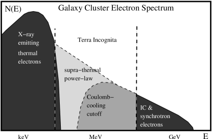
Figure 1: Sketch of the possible electron population in a galaxy cluster containing a radio halo in double logarithmic units. We have knowledge of the thermal (keV) and of the high energy (GeV) electron population due to their radiation. The intermediate region is yet terra incognita for our instruments. The sketched possible spectral shapes in this region are discussed in the text.

Clusters of galaxies contain thermal electrons with a temperature of several keV in the ICM. Several clusters also contain electrons with energies of several GeV, as demonstrated by the presence of cluster radio halos (Feretti & Giovannini, 1996; Feretti, 1999, for observational reviews). The origin of these high energy electrons is still a mystery. Several theories have been proposed (Enßlin, 1999b, for a review) such as electron injection by radio galaxies Jaffe (1977); Rephaeli (1977, 1979); Valtaoja (1984), in-situ electron (re-)acceleration by plasma- or shock-waves Jaffe (1977); Schlickeiser et al. (1987); Tribble (1993); Giovannini et al. (1993); Roettiger et al. (1993); Völk et al. (1996); Deiss et al. (1997); Roettiger et al. (1999); Sarazin (1999); Liang et al. (2000); Brunetti et al. (2001); Bykov et al. (2000); Takizawa & Naito (2000), and secondary particle injection after hadronic interactions of cosmic ray protons with the background gas Dennison (1980); Vestrand (1982); Blasi & Colafrancesco (1999); Dolag & Enßlin (2000).

The different scenarios lead to very different expectations for the electron spectrum in the unobserved intermediate energy range. In the in-situ acceleration scenario, the thermal and ultra-relativistic electron populations have to be connected by a supra-thermal population. The exact shape of this population depends on the details of the acceleration mechanism and the high Coulomb energy losses in this energy regime Dogiel (2000); Blasi (2000); Petrosian (2001). In Fig. 1 one possible realization of such a supra-thermal population is sketched. But if the electrons are injected with already high energies into the ICM, e.g. by escape from radio galaxies, or by hadronic secondary particle production, then the lower end of the intermediate energy range should be emptied by the rapid Coulomb energy losses, also sketched in Fig. 1. Further, additional spectral features can exist in this energy range, since the long electron cooling time of ICM electrons at 100 MeV allows the conservation of the imprints of earlier electron injection events for cosmological times Sarazin & Lieu (1998); Sarazin (1999).

1.3 Radio Galaxies

The activity phases of individual radio galaxies, as they appear to our instruments, are short-lived phenomena compared to cosmological time-scales. After a few ten million years the central engine in the galactic center ceases to power the radio cocoon (‘radio lobe’ in the radio astronomical jargon), and the observable radio emission vanishes rapidly Alexander & Leahy (1987); Komissarov & Gubanov (1994); Venturi et al. (1998); Slee & Roy (1998). The lifetime of very low frequency emission (0.01-10 MHz) from radio galaxies should be much longer than at higher frequencies, due to the strong energy-dependence of the radiative lifetimes of ultra-relativistic electrons.

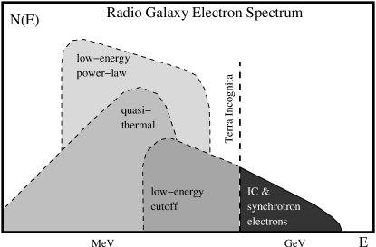
Figure 2: Sketch of the electron population in a radio galaxy in double logarithmic units. Several spectral features in the unobserved low energy range are shown. These are a low energy cutoff to the extrapolated observed spectrum and two possible distributions which are not usually discussed in the literature: a quasi thermal component and a separate low energy power law distribution.

The electron energy range below 100 MeV is practically unexplored yet. These electron have very long lifetimes, and they can be present a long time after the initial radio galaxy has stopped its activity Enßlin & Kaiser (2000), since both their IC radiation and very low frequency synchrotron emission do not cool them efficiently. Coulomb losses are also expected to be small, because of the very low density a possible thermal component must have in order to be consistent with the absence of the Faraday depolarization effect in radio cocoons Feigelson et al. (1995).

Some possible low-energy electron spectra of radio galaxies are sketched in Fig. 2. It could be that the power-law radio electron spectrum continues into the unobserved energy range, and then just has a cutoff. Such a low energy cutoff at an energy corresponding to an emission frequency of 10 MHz is usually assumed in the radio astronomical literature in order to calculate equipartition energy densities from the observed radio emission. This traditional cutoff at the frequency of the observational frontier gives equipartition energy densities which are within the order of magnitude range of reasonable values expected on other grounds. But it has to be noted that a systematic comparison of equipartition pressure of radio galaxies with their surrounding ICM pressure indicates that the former might be too low by a factor between 5 and 10 Feretti et al. (1990, 1992, 1995). If, in addition to this pressure discrepancy, radio galaxies are in fact over-pressured compared to their environments, as many source evolution scenarios require (Begelman & Cioffi, 1989; Kaiser & Alexander, 1997; Kaiser et al., 1997; Blundell et al., 1999, for example), then there is plenty of space for a large low-energy electron population and possibly protons, too.

Such an electron population could have a relativistic Maxwell-Boltzmann distribution, or a separate power-law from an earlier particle acceleration phase, e.g. within the radio jets of the radio galaxy. These possibilities are sketched in Fig. 2, and many others are possible since our knowledge about the dissipation processes of relativistic flows in jets are very limited. If mixing of the radio plasma with the ambient medium occurs, even a non-relativistic thermal population could be built up with time within the radio plasma volume.

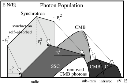
Figure 3: Sketch of the SSC and CMB-IC processes caused by a power-law electron momentum spectrum from $p_{1}$ to $p_{2}$. Shown are the synchrotron and CMB target photon distributions (the CRB is neglected for graphical clarity), the resulting IC scattered SSC and CMB-IC spectra, and the initial spectrum of the removed, up-scattered CMB photons. The latter will be recognized as negative flux by any differentially measuring CMB experiment. The arrows indicate how the corresponding features in the target and scattered photon spectra are related to the electron lower and upper cutoff momenta. For further explanations see the text.

1.4 Radio Ghosts

Powerful radio galaxies were a hundred times more abundant at higher redshifts. Therefore their fossils must be a ubiquitous ingredient of the present Universe, the radio ghosts Enßlin (1999a). Some of radio ghost’s possibly observable consequences would be their IC signature on the CMB due to their relativistic electron populations Enßlin & Kaiser (2000), and the scattering and isotropization of ultra-high energy comic rays by their magnetic fields Medina-Tanco & Enßlin (2001).

Indications that radio ghosts indeed exist are the detections of cavities in the X-ray emitting intra-cluster gas of the Perseus cluster Böhringer et al. (1993), the Cygnus-A cluster Carilli et al. (1994); Fabian et al. (2000), the Hydra-A cluster McNamara et al. (2000), Abell 2597 McNamara (2001), Abell 4059 Huang & Sarazin (1998); Heinz et al. (2001), Abell 2199 Fabian (2001), close to M84 in the Virgo Cluster Finoguenov & Jones (2001) and RBS797 Schindler et al. (2001). Whereas in most of these cases the cavities are obviously the radio cocoons of a radio galaxy at the cluster center, in some clusters also cavities without detectable radio emission were found, in Perseus and in Abell 2597 even close to cavities with detected radio emission. This fits nicely into the picture that the radio plasma outflows of radio galaxies fill subvolumes of the IGM, which are separated from the X-ray gas. It shows further that these cavities stay intact even after the observable radio emission has ceased, as one expects for the radio ghosts.

Further evidence of the existence of radio ghosts is given by the so called cluster radio relics. The properties of these sources can be understood in the context of cluster merger shock waves compressing fossil radio plasma clouds, and thereby re-ignite their observable synchrotron emission by the shock amplification of magnetic fields and electron energies Enßlin et al. (1998). The agreement between observed and theoretical spectra Enßlin & Gopal-Krishna (2001); Slee et al. (2001), morphologies, and polarization characteristics Enßlin & Brüggen (2001) supports this scenario and the existence of radio ghosts.

We consider below the SSC and CMB-IC spectra of radio ghosts at different redshifts because of the strong dependence of the high energy tail of the electron distribution on the CMB energy density.

1.5 Structure of the Paper

We give a brief overview about the basic physics in Sect. 2. The details of the formalism used can be found in the Appendixes. In Appendix A the radiative cooling of an electron population is investigated, in Appendix B synchrotron emission and absorption are described, and Appendix C deals with the IC and SSC processes.

This formalism is applied to study the spectral evolution of the SSC emission, and the IC scattered CMB and CRB for a set of characteristic radio sources in Sect. 4: powerful radio galaxies, like Cygnus A (Sect. 4.1), GPS (Sect. 4.2), giant radio galaxies (Sect. 4.3), the fossil radio plasma possibly released by our own galaxy (Sect. 4.4), and radio halo containing clusters of galaxies, like the Coma cluster (Sect. 4.5). Our main findings are summarized in Sect. 5.

2 The Basic Physics

2.1 Formalism & Approximations

We use monochromatic approximations for the calculation of the synchrotron and the inverse Compton radiation. This gives accurate results for the power-law regimes, but surely will be a crude approximation close to spectral cutoffs. But the uncertainties in the assumed model parameters do not require a higher accuracy in our illustrative treatment. Our treatment is not affected by the possible presence of a relativistic proton component in the radio plasma, since the model parameters were chosen on the basis of the observed radio flux. Synchrotron absorption of internal and external radiation fields is taken into account. The effect of the plasma frequency, and also the Tsytovich-Razin Tsytovich (1951); Razin (1960), the free-free, and induced Compton Sunyaev (1971) absorption low frequency cutoffs of the source internal synchrotron radiation field are neglected. This is justified due to the very low expected thermal gas density in radio cocoons. And even in the much denser galaxy clusters these effects are only important below $\sim 10$ kHz due to the high cluster temperatures (Lang, 1999, for the relevant formulae). External free-free absorption of the resulting low frequency emission can affect the observed SSC spectra of radio plasma embedded in the interstellar medium of galaxies, as the GPS sources. But since we calculate the intrinsic source spectrum, we do not correct for this.

The details of the calculations are laid down in the Appendix. Similar and more sophisticated formalisms were derived and applied by many other authors (Marscher, 1977; Gould, 1979; Band & Grindlay, 1985, for example). But several details of the calculation presented in the Appendix are not – to our knowledge – yet reported in the literature: e.g. formulae for the exact number density (Eq. B) and total number (Eq. 38) of synchrotron photons within a spherically homogeneous source, the generality of having several electron populations which can be located in regions with differing magnetic field strengths, useful asymptotic correct approximations of the external IC and SSC fluxes as a function of optical depth, and the inclusion of the IC decrement in external radiation fields into such a theoretical framework.

2.2 The Spectral Shape

In the following we give a qualitative discussion of the properties of the processes involved. This should clarify, for example, how our model spectra would change if different parameters were assumed.

Figure 4: Central surface brightness of our example radio cocoon (see Sect. 2.5). The synchrotron (long-dashed) and SSC+IC spectra (solid) are shown for power-law normalization parameter $C=3\cdot 10^{-8},\,10^{-7},\,3\cdot 10^{-7},\,10^{-6},\,3\cdot 10^{-6},\,10^{-5},\,\mbox{and}\,3\cdot 10^{-5}\,{\rm cm^{-3}}$ from bottom to top. The thick lines mark the case with our reference model with normalization $C=10^{-6}\,{\rm cm^{-3}}$. In spectral regions, where the SSC+IC processes lead to a reduction of the sky brightness below the CMB brightness, the absolute value of the (negative) SSC+IC surface brightness is plotted by a dotted line. The short-dashed line is the CMB spectrum. The dotted power-law line at frequencies below 1 GHz is the cosmic radio background (CRB). [Reference model parameters: $R=100$ kpc, $B=5\,\mu$G, $p_{1}=10$, $p_{2}=10^{3}$, $s=2$, $C=10^{-6}\,{\rm cm^{-3}}$].

For the moment, we assume a power-law (in momentum) relativistic electron distribution (per volume) with normalization $C$, spectral index $s$ and lower and upper cutoffs $p_{1}$ and $p_{2}$:

$$f(p)\,dp\,dV=C\,p^{-s}\,\Theta(p-p_{1})\,\Theta(p_{2}-p)\,dp\,dV$$ (1)

$\Theta(x)$ is the Heaviside step-function, so that for dimensionless electron momenta $p=P_{\rm e}/(m_{\rm e}\,c)$ ($P_{\rm e}$ is the electron momentum) outside $p_{1}<p<p_{2}$ the electron spectrum vanishes. We decided to use the dimensionless momentum $p$ rather than the canonical $\gamma$ in order to parameterize our electron spectra, since particle acceleration theories usually predict power law spectra in momentum rather than in kinetic energy, and the adiabatic losses and gains are also best described in momentum. In the ultra-relativistic limit $p$ and $\gamma$ are identical.

If located in a magnetic field with strength $B$, these electrons produce a synchrotron photon population between the frequencies

$$\nu_{{\rm s},1/2}=3\,e\,B\,p_{1/2}^{2}/(2\,\pi\,m_{\rm e}\,c)=\Lambda\,B\,p_{1/2}^{2}\,,$$ (2)

where the term $\Lambda=3\,e/(2\,\pi\,m_{\rm e}\,c)$ is introduced for convenience. As sketched in Fig. 3 the synchrotron spectrum consists (with increasing frequency) of an optically thick (synchrotron self-absorbed) low frequency part, and a decreasing optically thin high frequency part (for positive $s$). The internal synchrotron photons, and also the external CMB and CRB photons are partly scattered by the electron population to higher energies. This is also displayed in Fig. 3.

Figure 5: The strong dependence of SSC+IC spectra (solid) on the low energy cutoff in the electron distribution. The reference model with $p_{1}=10$ is plotted with thick lines. The curves are labeled with the electron lower momentum cutoff $p_{1}$. A CMB decrement occurs around 100 GHz in the $p_{1}=1$, and $p_{1}=10$ models, and below 50 GHz in the $p_{1}=100$ model. The latter is mostly an artifact of our monochromatic approximation, since it would be partly erased in a calculation in which the spectral width of the synchrotron and IC emission is taken into account. For further details see Fig. 4 and Sect. 2.5. [Reference model parameters: $R=100$ kpc, $B=5\,\mu$G, $p_{1}=10$, $p_{2}=10^{3}$, $s=2$, $C=10^{-6}\,{\rm cm^{-3}}$].

Ultra-relativistic electrons of momentum $p$ scatter photons with frequency $\nu$ to typically $\nu^{\prime}=\frac{4}{3}\,p^{2}\,\nu$. The SSC spectrum therefore extends from $\nu_{{\rm ssc},1}=\frac{4}{3}\,\Lambda\,B\,p_{1}^{4}$ to $\nu_{{\rm ssc},2}=\frac{4}{3}\,\Lambda\,B\,p_{2}^{4}$. If the synchrotron and the SSC cutoff of a source can be identified (or any other feature in these spectra caused by a peculiarity in the electron spectrum), the magnetic field strength of the source is immediately known:

$$B=\frac{4\,\nu_{{\rm s},2}^{2}}{3\,\Lambda\,\nu_{{\rm ssc},2}}\,.$$ (3)

The peak of the synchrotron spectrum translates into a similar peak in the SSC spectrum if the electron number spectrum has itself a distinctive peak. For steep power-law spectra, as mostly considered in this work, this is always the lower energy cutoff region. Therefore the synchrotron peak frequency gets shifted by a factor $\frac{4}{3}\,p_{1}^{2}$ to higher frequencies. This allows to derive the low energy cutoff of the electron spectrum from observing both, the synchrotron and the SSC peak. Or vice versa, a change of the cutoff parameter $p_{1}$ in one of our models results in a shift of the SSC peak location, without a significant change at higher frequencies. If $p_{1}$ is reduced, the high frequency SSC power law has to be continued at its low frequency end. The low frequency SSC spectrum below the IC scattered synchrotron self-absorption peak would increases correspondingly. A similar statement is true for the peak of the CMB-IC spectrum. An illustration of these effects is given by Fig. 5.

2.3 Timescales

The lifetime of particles radiating at a given frequency is significantly greater for the SSC process than for synchrotron emission. If only synchrotron and IC cooling are important, the cooling time at momentum $p$ is

$$t_{\rm cool}(p)=(a_{0}\,(u_{B}+u_{C})\,p)^{-1}\,,$$ (4)

where $a_{0}=\frac{4}{3}\,\sigma_{\rm T}/(m_{\rm e}\,c)$, and $u_{B}$ and $u_{C}$ are the magnetic and photon (mainly CMB) energy density. Therefore, the typical lifetimes at a given frequency $\nu$ are

$$t_{{\rm s}}(\nu)=\frac{({\nu}/({\Lambda\,B}))^{-\frac{1}{2}}}{a_{0}\,(u_{B}+u_{C})}\ll t_{{\rm ssc}}(\nu)=\frac{({3\,\nu}/({4\,\Lambda\,B}))^{-\frac{1}{4}}}{a_{0}\,(u_{B}+u_{C})}\,.$$ (5)

The ratio of the lifetimes is only weakly dependent on the magnetic field strength and the frequency itself:

$$\frac{t_{\rm ssc}(\nu)}{t_{\rm s}(\nu)}=\left(\frac{4\,\nu}{3\,\Lambda\,B}\right)^{\frac{1}{4}}=112\,\left(\frac{\nu}{\rm GHz}\right)^{\frac{1}{4}}\,\left(\frac{B}{\mu\rm G}\right)^{-\frac{1}{4}}$$ (6)

As a rule of thumb, the SSC flux lasts two orders of magnitude longer than the synchrotron emission, if only synchrotron and IC losses are important. This should apply for galaxy cluster radio halos and their descendent electron populations, but usually not for radio galaxies which are still expanding and therefore have strong adiabatic losses.

Figure 6: Redshift dependence of the SSC+IC spectra. Displayed is the central surface brightness of our example radio cocoon [$R=100$ kpc, $B=5\,\mu$G, $p_{1}=10$, $p_{2}=10^{4}$ (!), $s=2$, $C=10^{-6}\,{\rm cm^{-3}}$] for redshifts $z=0$, $z=1$, and $z=3$. For further details see Fig. 4 and Sect. 2.5.

2.4 Luminosities

The synchrotron, SSC, and CMB-IC luminosities scale differently with the source properties. The SSC luminosity depends very sensitively on the source internal energy density. The synchrotron luminosity also strongly depends on the source energy density, but to a lower degree than the SSC luminosity. The CMB-IC luminosity is least dependent. This is illustrated in Fig. 4.

Adiabatic compression of the source volume $V$ by a factor $\tilde{C}$ changes the electron spectrum ($f(p)\,dp\,dV$) normalization by $C\propto\tilde{C}^{({s+2})/{3}}$, and the magnetic field strength by $B\propto\tilde{C}^{{2}/{3}}$. In the optically thin power-law regime, the synchrotron luminosity scales like

$$L_{\rm s}(\nu)\propto V\,C\,B^{\frac{s+1}{2}}\propto\tilde{C}^{\frac{2s}{3}}$$ (7)

(Eq. 33), the SSC luminosity with

$$L_{\rm ssc}(\nu)\propto V^{\frac{4}{3}}\,C^{2}\,B^{\frac{s+1}{2}}\propto\tilde{C}^{\frac{3s+1}{3}}$$ (8)

(Eq. 54), and the CMB-IC (or similar CRB-IC) luminosity scales like

$$L_{\rm CMB-IC}(\nu)\propto V\,C\propto\tilde{C}^{\frac{s-1}{3}}$$ (9)

(Eq. 48). If the compression of a radio plasma cocoon is due to an environmental pressure change from $P_{1}$ to $P_{2}$, e.g. in a cluster merger shock wave, the adiabatic relation of relativistic plasma $(P_{2}/P_{1})=\tilde{C}^{{4}/{3}}$ leads to $L_{\rm s}\propto(P_{2}/P_{1})^{{s}/{2}}$, $L_{\rm ssc}\propto(P_{2}/P_{1})^{({3s+1})/{4}}$, and $L_{\rm CMB-IC}\propto(P_{2}/P_{1})^{({s-1})/{4}}$. From this, one sees that synchrotron and SSC emission are strongly, but CMB-IC luminosity is only weakly affected by compression. The spectral distortions in the CMB frequency range by the CMB-IC process is mostly an absorption feature due to the removed, up-scattered photons. Its strength depends only on the total number of ultra-relativistic electrons, and is therefore completely independent of the compression state of the radio plasma Enßlin & Kaiser (2000).

Figure 7: As Fig. 6, but after 100 Myr of radiative cooling. The $z=3$ model’s remaining synchrotron emission is at too low frequencies to be displayed.

2.5 Particular Examples

In order to demonstrate the richness of information contained in the SSC + CMB-IC spectra we investigate the following example: the radius of an old radio cocoon is assumed to be 100 kpc, the magnetic field strength $B=5\,\mu$G, the power-law electron spectrum extends from $p_{1}=10$ to $p_{2}=1000$ with a spectral index $s=2$ and a normalization of $C=10^{-6}\,{\rm cm^{-3}}$.

The spectrum of this cocoon is displayed in Fig. 4, together with similar models where the electron spectrum normalization $C$ is varied (partially to unrealistic values). Since synchrotron and CMB-IC spectra are proportional to $C$, but the SSC spectrum is proportional to $C^{2}$ the total source spectrum change its shape significantly with a variation of $C$. A CMB-IC decrement centered on $\sim 100$ GHz appears for sufficiently low normalizations of the electron spectrum.

In Fig. 5 different models are displayed, where now the low energy cutoff is changed. A strong dependence of the resulting spectra on this cutoff is obvious. With decreasing $p_{1}$ the electron number density strongly increases and the CMB-IC decrement (increment) becomes dominant around 100 GHz (above 1 THz). Also the SSC emission at low radio frequencies increases with decreasing $p_{1}$.

In Fig. 6 the model cocoons (here with $p_{2}=10^{4}$) are located at different redshifts ($z=0,1,3$). The CRB co-moving photon density is assumed to be reduced to 50% at $z=1$, and 10% ($z=3$) compared to its present value. Since the synchrotron and SSC brightnesses suffer from the cosmological redshift, but the CMB-IC flux does not, a high redshift source can have a qualitatively very different SSC + CMB-IC spectrum compared to its low redshift counterpart. In addition to this, after the shutdown of the radio jets, these differences are further amplified by the action of radiative cooling, which is stronger at higher redshifts. This is illustrated by Fig. 7, where the spectra of our models are shown after 100 Myr cooling.

With Fig. 8 we demonstrate that the combined SSC and CMB-IC spectra contain enough information in order to discriminate between models with different energy-rich low energy electron populations, e.g. power-law and relativistic Maxwell-Boltzmann distributions (Eq. 17) as e.g. sketched in Fig. 2.

Figure 8: The dependence of SSC+IC spectra in the case of presence of additional components of low energy relativistic electrons. The thick lines mark the case with our reference model. 1) The upper solid line is with an additional power-law component ($p_{1}=1$, $p_{2}=10$, $s=2$, $C=10^{-6}\,{\rm cm^{-3}}$ which is a 10 times higher normalization than at higher energies). 2) The dot-dashed lines are models with added relativistic thermal populations with the same amount of kinetic energy as the additional power-law model ($kT_{\rm e}=1\,m_{\rm e}\,c^{2}$ with $n_{{\rm e},{\rm th}}=8.4\cdot 10^{-6}\,{\rm cm^{-3}}$ and $kT_{\rm e}=3\,m_{\rm e}\,c^{2}$ with $n_{{\rm e},{\rm th}}=2.8\cdot 10^{-6}\,{\rm cm^{-3}}$, see Eq. 17). For further details see Fig. 4. [Reference model parameters: $R=100$ kpc, $B=5\,\mu$G, $p_{1}=10$, $p_{2}=10^{3}$, $s=2$, $C=10^{-6}\,{\rm cm^{-3}}$].

Instrument	Frequency	Sensitivity	FWHM	http://
LOFAR	10-300 MHz	$\sim$ mJy	$20^{\prime\prime}-1^{\prime\prime}$	rsd-www.nrl.navy.mil/7213/lazio/decade_web
LOFAR core	10-300 MHz	$\sim$4 mJy	$50^{\prime}-3^{\prime}$	rsd-www.nrl.navy.mil/7213/lazio/decade_web
GMRT	0.1-1 GHz	150-30 $\mu$Jy	$20^{\prime\prime}-2^{\prime\prime}$	www.ncra.tifr.res.in/ncra_hpage/gmrt/gmrt_spec.html
GMRT core	0.1-1 GHz	300-60 $\mu$Jy	$7^{\prime}-0.7^{\prime}$	www.ncra.tifr.res.in/ncra_hpage/gmrt/gmrt_spec.html
ATA	1-10 GHz	30 $\mu$Jy	$75^{\prime\prime}-9^{\prime\prime}$	astron.berkeley.edu/ral/ATAImagerDocs.html
EVLA	1-50 GHz	2-20 $\mu$Jy	$3^{\prime}-0.1^{\prime}$	www.aoc.nrao.edu/doc/vla/EVLA
ALMA	35-850 GHz	2-450 $\mu$Jy	$10^{\prime\prime}-0.5^{\prime\prime}$	www.eso.org:8082/info/sensitivities/index.html
PLANCK LFI	30-100 GHz	13-27 mJy	$33^{\prime}-10^{\prime}$	astro.estec.esa.nl/Planck/technical/payl/node6.html
PLANCK HFI	0.1-0.9 THz	10-40 mJy	$11^{\prime}-5^{\prime}$	astro.estec.esa.nl/Planck/technical/payl/node7.html
HERSCHEL	0.4-4 THz	$\sim$ mJy	$\sim 10^{\prime\prime}$	astro.estec.esa.nl/astrogen/first/experiments_frame.html

Table 1: Technical specifications of planed instruments (1st row), as advertised on their Internet pages (5st row): observing frequencies (2st row), 1-sigma point source sensitivity (3rd row), and beam FWHM (4th row). Sensitivities are given for 1 h observation, except in the case of the PLANCK instruments, where they are given for the completed PLANCK survey. For the EVLA and ALMA the compact array configurations were assumed. Note, that most of these instruments are still under design, so that the values given here may become obsolete.

2.6 Polarization

IC scattering of an anisotropic seed photon field leads to some polarization in the scattered radiation for small electron Lorentz factors (see e.g. Begelman et al. Begelman et al. (1987)). In our spherically symmetric model the photon field has a radial anisotropy at off-center locations. Therefore the source should exhibit an SSC polarization pattern, which is strongest at the source edge and has electric vectors aligned on circles. The source averaged polarization is zero in our highly symmetric toy model. But in nature, typical sources can be expected to be elongated. For radio galaxy lobes, elongation by a factor of two are not unusual, and rather large aspect ratios can be attributed to head-tail radio galaxies. Thus, we expect radio galaxies to exhibit a small level of linearly polarized SSC flux at lowest frequencies due to source elongation, if a substantial only mildly relativistic electron population is present in the source.

Further, the intrinsic synchrotron polarization of sources with large-scale ordered magnetic fields is conserved to a large fraction in the IC process Bonometto & Saggion (1973); Celotti & Matt (1994). Since many radio galaxies exhibit polarization, fossil radio galaxies should often have an intrinsically polarized SSC flux of up to 40 % polarization at all frequencies.

Environmental influences on the radio plasma, like shear flows and shock compression, can increase both polarization effects by increasing the source elongation and by aligning the internal magnetic fields (Enßlin & Brüggen, 2001, for the impact of shock waves).

Very peculiar polarization properties can arise around 100 GHz for sources, where the unpolarized CMB is diminished by IC scattering, but polarized SSC emission contributes to this spectral range. If the CMB-IC decrement exceeds the SSC luminosity a polarized decrement in the CMB sky can be found at these frequencies. This can be of importance for future high precision CMB polarization measurements.

3 Upcoming Instruments

Several telescopes are under development which may be suitable to search for SSC and CMB-IC signatures of low energy cosmic ray electrons. We list in Tab. 1 approximate values of expected point source sensitivities $F_{\nu}$ of several planed instruments. If a source with surface brightness $S_{\nu}$ and angular area $A_{\rm s}$ is smaller or comparable to the instrument beam with area $A_{\rm b}$ then the full sensitivity can directly be compared to the source luminosity in order to estimate the significance $\sigma$ of the expected detection: $\sigma\approx S_{\nu}\,A_{\rm s}/F_{\nu}$. If the source appears extended the significance is lower. For a single-dish and phased array telescopes the significance is approximately given by $\sigma\approx S_{\nu}\,(A_{\rm s}\,A_{\rm b})^{1/2}/F_{\nu}$, since the signal of the $N=A_{\rm s}/A_{\rm b}$ individual beams should be added like independent measurements yielding $\sigma_{\rm total}\approx\sigma_{\rm beam}\,N^{1/2}$. For interferometers, the detected signal of an extended source scales with (the square root of) the fraction of the telescope baselines for which the source is still unresolved. This depends strongly on the individual array design and we therefore do not attempt to estimate it. Often, the interferometers elements are distributed in a way that many more short baselines (which are sensitive to large-scale structures) exist than long baselines (which only see small angular sources). For example it is planed that $\approx 25$% of the collecting area of LOFAR is within a virtual core of 2 km diameter (compared to an instrument diameter of 300 km). Therefore the virtual core of LOFAR is quiet sensitive to extended flux on angular scales 60 times larger than the full resolution of the instrument.

4 Astrophysical SSC Sources

In the following models of several extragalactic SSC and CMB-IC sources are discussed. The exact definitions of the model parameters can be found in the Appendix. We give hints on the detectability of theses sources by the instruments listed in Tab. 1 based on rough detection significance estimates as described in Sect. 3.

4.1 Cygnus A-like Radio Galaxies

Figure 9: Central surface brightness of our Cygnus A-like radio cocoon in a cooling and expanding phase. It is assumed that the radio plasma supply was shut down in a stage corresponding to the present Cygnus A stage and the radio cocoon expanded afterwards during its buoyant rise in the cluster atmosphere. The synchrotron (long-dashed) and SSC+IC spectra (solid) are shown for the stages at the jet-power shutdown, and for stages 20, 40, 80, 120, 160, and 200 Myr after this. In spectral regions, where the SSC+IC processes lead to a reduction of the brightness below the CMB brightness, the absolute value of the (negative) SSC+IC surface brightness is plotted by a dotted line. The top one of the short-dashed lines is the CMB spectrum. The short-dashed lines below this is the CMB spectrum multiplied by diminishing factors of $10^{-2},10^{-4},10^{-6},10^{-8},\,\mbox{and}\,10^{-10}$ in order to allow a convenient read off of the relative source brightness expressed in terms of the CMB brightness at the same frequency. The dotted power-law line at frequencies below 1 GHz is the cosmic radio background (CRB). [Model parameters: $R=20$ kpc, $B=35\,\mu$G, $p_{1}=10$, $p_{2}=3\cdot 10^{4}$, $s=2.4$, $C=6.63\cdot 10^{-4}\,{\rm cm^{-3}}$, $b=1.5$, $t_{0}=75$ Myr].

Our high luminosity radio galaxy is assumed to have spherical lobes with a diameter of 40 kpc, and a magnetic field strength of 35 $\mu$G. The electron population is a single power-law with spectral index of $s=2.4$, which extends from $p_{1}=10$ to $p_{2}=3\,\cdot 10^{4}$ and which is normalized by $C=6.63\cdot 10^{-4}\,{\rm cm}^{-3}$. This corresponds to an energy content in relativistic electrons of $4.9\cdot 10^{59}$ erg and in magnetic fields of $4.8\cdot 10^{58}$ erg. The energy ratio of electronic to magnetic energy is 10, and therefore by only a factor of a few above what radio-astronomers call equipartition, for which the energy of electrons radiating above 10 MHz equals that of the magnetic fields. The luminosity at 1 GHz is $3.9\cdot 10^{34}\,{\rm erg/Hz/s}$. Cygnus A, for example, has a flux of 214 Jy at 8 GHz Stull (1971), as two of our model cocoons if they are placed at the luminosity distance of 265 Mpc, similar to that of Cygnus A for $H_{0}=65\,{\rm km/s/Mpc}$ and $q_{0}=0.5$ (Owen et al., 1997, for the redshift). The synchrotron and SSC central surface brightness of our radio cocoons are shown in Fig. 9.

Figure 10: Central brightness of our GPS model. Although the surface brightness appears to be very high, the typical $10^{-1}...10^{-2}$ arcsec sizes of GPS imply a few Jy apparent luminosity at their spectral peak. The spectra are displayed for a fresh GPS (top), and for possible later stages 0.017, 0.033, 0.050, 0.067, 0.083, and 0.1 Myr after a (hypothetical) jet-power shutdown. For further explanations see Fig. 9. [Model parameters: $R=0.05$ kpc, $B=1\,$mG, $p_{1}=10$, $p_{2}=3\cdot 10^{4}$, $s=2.1$, $C=0.3\,{\rm cm^{-3}}$, $b=1.5$, $t_{0}=0.003$ Myr].

In this figure possible later stages in the evolution of the radio source, after the supply with fresh electrons was shut down, are also shown. In order to model these stages we assume that the radio cocoons will expand adiabatically while they rise buoyantly in the cluster atmosphere Churazov et al. (2001); Brüggen & Kaiser (2001). In our illustrating example we assume that the jet supply of fresh radio plasma shuts down at the present evolutionary stage of Cygnus A. The two radio cocoons are assumed to expand with $b=3/2$ and $t_{0}=75$ Myr (see Eq. 12). This should serve as a rough model for a rise with half sonic velocity in a singular isothermal cluster atmosphere (cluster density $\propto$ cluster radius^-2). We note that the evolution of the electron spectra is not corrected for the reduced synchrotron cooling at self absorbed frequencies. An investigation of this more complicated problem was done by Rees Rees (1967)

It is obvious, that a radio cocoon of a powerful, compact radio galaxy produces a detectable SSC flux for a long time after the the synchrotron radio emission vanished from the radio observable frequency band. At low radio frequencies the SSC flux remains even for a few Gyr, due to the slow energy losses by self-absorbed synchrotron emission. But adiabatic losses due the expansion of the source are able to reduce the SSC flux substantially.

The typical angular area is of the order of arcmin². Therefore all of the instruments listed in Tab. 1 should be able to detect a Cygnus-A like radio cocoon. All but LOFAR and GMRT see it best shortly after the decay of the synchrotron emission. The latter is because at below GHz frequencies the source emission is rising with time during the first few 100 Myr. PLANCK and HERSCHEL should give only relative week detection of early stages. However, if such a very powerful radio ghost would be much closer, e.g. located in the Virgo cluster, even later stages may be detectable with these instruments.

4.2 GHz Peak Sources

GPS are believed to be the very early stage of radio galaxies, in which a small ($<$ kpc) radio cocoon is working its way through the dense interstellar medium of a radio galaxy (Snellen et al., 2000; De Zotti et al., 2000, and references therein). The spectral peak at typically a GHz is likely due to synchrotron-self-absorption at lower frequencies. Although it turns out that SSC emission of GPS is very weak and practically unobservable, we briefly discuss such sources for completeness since they are another extreme case of radio galaxies.

The SSC flux of GPS should exhibit a peak around 100 GHz $(p_{1}/10)^{2}$, where $p_{1}$ is the minimum electron momentum of the population. A detection of such a peak would give deep insight into the low energy end of the relativistic electron population. Unfortunately, the synchrotron flux will likely also dominate this spectral regime, unless there is a relatively low high energy cutoff in the electron spectrum. Even in that case the brightness will be only of the order of the CMB, which gives a very low signal for these small-scale sources.

As an illustration, we have chosen the following parameters of our model GPS: $R=0.05$ kpc, $B=1$mG, $C=0.3\,{\rm cm^{-3}}$, $s=2.1$, $p_{1}=10$, and $p_{2}=3\cdot 10^{4}$. This source peaks around 0.3 GHz and has a GHz luminosity of $1.4\cdot 10^{33}\,{\rm erg\,s^{-1}\,Hz^{-1}}$, as it is typical for GPS sources. The synchrotron and SSC spectra are shown in Fig. 10, together with spectra for hypothetical later stages, after a shutdown of the central engine. We assumed for this phase $t_{0}=0.03$ Myr, and $b=1.5$ (see Eq. 12).

The SSC flux can easily extend into the gamma ray regime, but the total luminosity is very low with $\nu L_{\nu}\sim 10^{34...35}\,{\rm erg\,s^{-1}}$ in the X-ray to gamma ray regime. Thus, GPS are not expected to be easily detectable via their SSC flux.

4.3 Giant Radio Galaxies

Figure 11: Central surface brightness of our giant radio galaxy radio cocoon. Here a compression scenario was assumed, so that the radio luminosity at low frequencies, and the IC & SSC flux at most frequencies increases with time. Spectra are displayed for the jet shutdown time and 0.3, 0.6, 1.2, 1.8, 2.4, and 3 Gyr after this. For further explanations see Fig. 9. [Model parameters: $R=400$ kpc, $B=1\,\mu$G, $C=5\cdot 10^{-7}\,{\rm cm^{-3}}$, $s=2.5$, $p_{1}=10$, $p_{2}=3\cdot 10^{4}$, $b=-1$, $t_{0}=500$ Myr].

Giant radio galaxies are an other extreme class of powerful radio galaxies. Their radio cocoons can have diameters of a Mpc, since they expand into a low density environment. Therefore, the magnetic and electron energy densities are expected to be much lower in these sources (Mack et al., 1997; Schoenmakers et al., 2000, for recent reviews).

Here, we adopt a radius of 400 kpc, a magnetic field strength of $1\,\mu$G, a single power law electron population with spectral index $s=2.5$, and a normalization of $C=5\cdot 10^{-7}\,{\rm cm^{-3}}$. As in the case of Cygnus A, we assume $p_{1}=10$ and $p_{2}=3\cdot 10^{4}$. Since the cooling is CMB-IC dominated, optical thickness of the synchrotron radiation does not change these cooling ages. The magnetic and electronic energies of this cocoon are $3\cdot 10^{59}$ erg and $2\cdot 10^{60}$ erg. The luminosity of the cocoon is $2\cdot 10^{32}\,{\rm erg\,s^{-1}Hz^{-1}}$ at 1 GHz, corresponding to a flux of 18 Jy at 1 GHz and 100 Mpc luminosity distance.

The radio emission typically disappears on a 100 Myr time-scale after the jet-power is shut down, but the IC and SSC flux remain for Gyrs. Expansion of the fossil radio cocoon would nearly completely diminish these already weak fluxes. But compression can strongly increase the SSC flux even at very late stages. This is shown in Fig. 11, where a compression, described by $b=-1$ and $t_{0}=500$ Myr (see Eq. 12), was assumed. Within the displayed 3 Gyr evolution a compression of a factor $\tilde{C}=7$ is reached. Although the compression here is artificially introduced, it should illustrate the consequences of the growth of structures like groups and filaments of galaxies in which many fossils of giant radio galaxies are expected to be embedded.

The expected angular area of a giant radio galaxy ghost is of the order of 300 arcmin². However, only the GMRT, EVLA, and ATA telescopes (out of the sample listed in Tab. 1) at GHz frequencies have reasonable chances to detect such a source. And this only if it is either environmentally compressed or if extremly long integration times are used ($10^{2}-10^{3}$ h).

4.4 The Nearest Radio Ghost

Figure 12: Central surface brightness of a possible radio ghost produced by our own galaxy. Also here a compression scenario was assumed, leading to a compression by a factor of 11 in 10 Gyr), so that the radio luminosity at low frequencies, and the IC & SSC flux at most frequencies increases with time until an age of 6 Gyr. After this the SSC flux declines again due to the rapidly decreasing electron high energy spectral cutoff. Spectra are displayed for the jet shutdown time and subsequent times of 1, 2, 4, 6, 8, and 10 Gyr after this (ignoring CMB redshift evolution for simplicity). For further explanations see Fig. 9. [Model parameters: $R=200$ kpc, $B=1\,\mu$G, $C=5\cdot 10^{-7}\,{\rm cm^{-3}}$, $s=2.5$, $p_{1}=10$, $p_{2}=3\cdot 10^{4}$, $b=-1$, $t_{0}=1$ Gyr].

The Milky Way or the Andromeda galaxy harbor very massive central black holes with masses of $2.6\cdot 10^{6}\,M_{\odot}$ Genzel et al. (1997) and $\sim 3\cdot 10^{7}\,M_{\odot}$ Kormendy & Bender (1999) respectively. If the growth of these black holes was due to feeding of gas from an accretion disk, it can be expected that this process was accompanied by a relativistic jet outflow. If 10 % of the rest-mass of the accreted gas was converted into jet-power, enough radio plasma should have been produced in order to fill an inter-galactic volume of the order of 0.1 Mpc${}^{3}\,(B/\mu{\rm G})^{-2}$ Medina-Tanco & Enßlin (2001) with outflows from our galaxy, and ten times as much with outflows from Andromeda. The term $B$ denotes here the equipartition magnetic field strength as a measure of the internal energy density. A moderately sized nearby radio ghost of this origin may have a radius of 200 kpc, a magnetic field strength of $1\,\mu$G, a single power law electron population with spectral index $s=2.5$, and an normalization of $C=5\cdot 10^{-7}\,{\rm cm^{-3}}$. As in the other cases of radio plasma, we assume $p_{1}=10$ and $p_{2}=3\cdot 10^{4}$. Similar to giant radio galaxies, one gets a very low SSC surface brightness, as displayed in Fig. 12. Synchrotron and IC cooling is not able to remove the flux within 10 Gyr. The brightness could increase drastically due to compression, if the environmental pressure grew considerably in the recent past due to accretion of matter onto the local group. If such a compressed fossil radio cocoon were nearby it would produce a relatively big total SSC flux due to its very large angular size ($\sim 100$ deg${}^{2}\sim 10^{6}$ arcmin²). Maybe ATA and GMRT would have a chance to detect this, if these telescopes would still be sensitive to such large scales. A detection by PLANCK should fail only by roughly one order of magnitude. This leaves some hope that a sensitive ground (or balloon) based single dish telescope is able to detect the large scale CMB decrement of the order of $10^{-8}-10^{-7}$ caused by such a nearby radio ghost.

Figure 13: The (central) electron spectrum in the Coma cluster of galaxies. The thick line is the thermal distribution and the assumed relativistic population. The upper limits result from observational upper limits to bremsstrahlung or IC scattering fluxes in various wave-bands. Two of them correspond to actual detections: the extreme ultraviolet (EUV) Lieu et al. (1996) and the high energy X-ray (HEX) excess fluxes Fusco-Femiano et al. (1999). Some of the corresponding upper limits (labeled by EUV and HEX) on the electron spectra could therefore be data points. The thin lines give the required electron populations in order to produce the observed radio halo of Coma with the labeled magnetic field strengths. For details see Enßlin & Biermann Enßlin & Biermann (1998).

Figure 14: Central surface brightness of the Coma-like galaxy cluster for the electron spectrum displayed in Fig. 13. Also displayed are spectra 1, 2, 3, 4, 6., 8., and 10 Gyr after the supply of fresh electrons stopped (ignoring CMB redshift evolution for simplicity). They are presented only as illustrations, since no evolution of the cluster is assumed for this period and Coulomb losses, which would quickly remove the low energy electrons, are also neglected. For further explanations of this figure see Fig. 9. [Model parameters: $R=400$ kpc, $B=1.2\,\mu$G, $C_{1}=9.34\cdot 10^{-7}\,{\rm cm^{-3}}$, $s_{1}=2$, $p_{1,1}=3$, $p_{1,2}=100$, $C_{2}=2.14\cdot 10^{-3}\,{\rm cm^{-3}}$, $s_{2}=3.68$, $p_{2,1}=100$, $p_{2,2}=3\cdot 10^{4}$].

4.5 Galaxy Clusters

Several clusters of galaxies host cluster wide diffuse radio emission, the ‘cluster radio halos’. The origin of the relativistic electrons producing the halos is not yet settled. They might be transient features or persistent. We model a Coma cluster type radio halo and follow its evolution after a hypothetical shut down of the supply of fresh relativistic electrons.

We approximate the cluster by a homogeneous sphere of 400 kpc radius. The field strength is assumed to be 1.2 $\mu$G, allowing the same population of electrons to produce the radio emission and the observed extreme ultra-violet excess by IC scattering of the CMB. The electron spectrum is described by a broken power-law: for $3<p<100$ we use $s_{1}=2$ and $C_{1}=9.34\cdot 10^{-7}\,{\rm cm}^{-3}$, and for $100<p<3\cdot 10^{4}$ we use $s_{2}=3.68$ and $C_{2}=2.14\cdot 10^{-3}\,{\rm cm}^{-3}$.

The ratio of relativistic electron to magnetic field energy density is of the order of 50. It is dominated by the low energy electrons, which are usually neglected in the calculation of equipartition magnetic fields from radio observations. The ratio of relativistic to thermal electron energy density in this model is moderate: $2.5\%$.

A compilation of the available information on the electron spectrum in Coma was given by Enßlin & Biermann Enßlin & Biermann (1998). Although a beta-profile was used in this work to model the electron and magnetic field distribution, our homogeneous sphere should give comparable emission for the same densities, sufficiently accurate for our purposes. We can therefore compare directly the above assumed electron spectrum with the observational limits resulting from various radiation processes in Fig. 13.

The spectrum of our model of the diffuse emission in Coma is shown in Fig. 14. The synchrotron/IC cooled spectra are also shown at times after the supply of high energy electrons has stopped. The low energy electron population is assumed to be preserved against Coulomb losses by re-acceleration or injection of electrons. This demonstrates that some weak SSC flux could come from clusters which do not exhibit observable synchrotron emission at all.

It should be noted that Coma is not at the upper end of the cluster radio halo luminosity distribution. The most luminous radio halo known to date in the cluster 1E 0657-56 is roughly 10 times brighter than Coma Liang et al. (2000). The expected SSC luminosity of this cluster is therefore expected to be more than an order of magnitude higher than in our model for Coma.

Coma’s relativistic electron population cover roughly 300 arcmin² of the sky. This may allow detection by LOFAR of an remnant of a radio halo in a nearby (Coma-like) cluster with very long integration times ($10^{2}-10^{3}$ h). But GMRT, ATA, and EVLA have very good chances of an detection at their lowest frequencies (0.1 GHz for GMRT, GHz for ATA and EVLA) of such an aged radio halo. Experiments in the CMB range should also come close to detection of the relativistic CMB decrement produced by fresh or aged radio halo electron populations, if they do not completely resolve out the source structure. Unfortunately, any detected signal is weak compared to the thermal Sunyaev-Zeldovich effect. In optimistic scenarios, a marginal discrimination of such a relativistic CMB decrement may still be possible even with PLANCK Enßlin & Kaiser (2000).

5 Conclusion

We have modeled SSC and IC spectra of different astrophysical sources under consideration of synchrotron self-absorption, electron aging by synchrotron, and IC losses, and adiabatic losses and gains. Although the SSC luminosity of a typical radio source is weak compared to its synchrotron luminosity, the SSC lifetime exceeds the synchrotron lifetime of the source by a large margin. This property can make the SSC emission an important probe of the fossil stages of former radio luminous galaxies. It allows further to probe the spectral shape of the low energy population of relativistic electrons of a source, which is otherwise not accessible. Since the SSC flux depends strongly on the energy density of the relativistic electrons and magnetic fields, it is a very sensitive probe of the compression state of the fossil radio plasma and therefore of its environment.

Powerful radio galaxies are expected to have the strongest SSC luminosities. Their fossil radio plasma clouds (radio ghosts) can be detectable even if adiabatic expansion is affecting them. Possible candidates for the detection are the recently discovered cavities in the X-ray gas of some clusters of galaxies. These are likely radio ghosts produced by the central cluster galaxy, which are currently on their buoyant rise through the cluster atmosphere. Examples are listed in Sect. 1.4. The best time to detect the SSC flux of a rising radio plasma bubble is during the first 100 Myr, before adiabatic expansion has diminished its luminosity.

Giant radio galaxies, which have very extended radio cocoons, and which are residing in low density environments, produce only a very low SSC surface brightness. Environmental compression of such a lobe would certainly help to make it detectable, even after a couple of Gyrs of lurking.

GHz peak sources have extreme SSC surface brightnesses, but very low luminosities due to their small angular extent. If at all, their SSC flux might be best detectable at X-ray or even gamma ray energies.

The nearest radio ghost may be produced by an earlier activity of the Milky Way’s or the Andromeda galaxy’s central black hole. Although its SSC surface brightness is expected to be very low, its large angular extent may give us a chance to detect it with single dish experiments at its expected emission peak in the range of 0.1-10 GHz or at its CMB decrement.

A Coma-like galaxy cluster is expected to produce SSC flux even a long time after a shut down of the process, which supplied the radio halo emitting electrons.

The detection of the SSC emission of one of these classes of sources is an observational challenge. It would be rewarded by insight into a formerly unseen electron population and into the fossil Universe of relativistic particle populations. Due to its broad frequency spectra, it can be probed with several future high sensitivity instruments, ranging from lowest radio frequencies GMRT and LOFAR, over microwave spacecraft MAP and PLANCK, balloon and ground based CMB experiments, and sub-mm/IR projects ALMA and HERSCHEL satellite, eventually even up into the X-ray and gamma-ray range. A multi-frequency sky survey, as will be provided by the Planck experiment, should allow to search for the SSC and relativistic IC spectral signature of many nearby clusters of galaxies and radio galaxies at least in a statistical way. In addition to this, there should be targeted observations of promising candidates, as e.g. the recently reported X-ray cluster cavities. We demonstrated that new and upcoming radio arrays with large collecting areas in the 0.1-1 GHz range as LOFAR, GMRT, EVLA and ATA have excellent detection chances. We hope that this work stimulates observational efforts to exploit the spectral landscape of the terra incognita of 1-100 MeV electrons residing in the intergalactic space via their combined SSC and CMB-IC emission.

The expected long-living SSC source population of fossil radio galaxies, and their possible impact on CMB experiments will be investigated in a separate forthcoming paper.

Appendix A Cooling Electron Spectra

We assume that the emission region is a homogeneous sphere with radius $R$. The magnetic fields are assumed to have isotropic orientations. Several electron populations with isotropic momentum distributions and power-law momentum spectra are assumed to exist simultaneously in the emission region. Initially, they are assumed to be power-law distributions:

$$f_{i}(p)\,dp\,dV=C_{i}\,p^{-s_{i}}\,\Theta(p-p_{1,i})\,\Theta(p_{2,i}-p)\,dp\,dV$$ (10)

The index $i$ labels the different spectra, which have normalizations of $C_{i}$, and spectral indices $s_{i}$. $\Theta(x)$ is the Heaviside step-function, so that for dimensionless electron momenta $p=P_{\rm e}/(m_{\rm e}\,c)$ outside $p_{1,i}<p<p_{2,i}$ the electron spectra vanish. The freedom to have several populations allows to model complex spectra with broken power-laws or spectral discontinuities. We also allow that each electron population is located within a different magnetic field strength $B_{i}$, so that small-scale multi-phase media can be modeled.

After the supply of fresh electrons has stopped, the electron spectra evolve according to synchrotron, IC, and adiabatic energy losses:

$$-\frac{dp}{dt}=a_{0}\,(u_{B}+u_{C})\,p^{2}+\frac{1}{3}\,\frac{1}{V}\,\frac{dV}{dt}\,p\,,$$ (11)

where $a_{0}=\frac{4}{3}\,\sigma_{\rm T}/(m_{\rm e}\,c)$, $V$ is the source volume, $u_{B}$ and $u_{C}$ are the magnetic and CMB energy densities respectively. We do not consider bremsstrahlung and Coulomb losses in view of the very low particle density in most of the considered sources. We assume that the expansion of the source volume can be described by a power-law in time:

$$V(t)=V_{0}\,\left({t}/{t_{0}}\right)^{b}=V_{0}/\tilde{C}(t)\,,$$ (12)

where $\tilde{C}(t)$ denotes the compression factor.

In this case the evolution of the momentum of an electron residing in a magnetic field strength $B_{i}(t)=B_{i}\,\tilde{C}^{2/3}$ can be given analytically (Kaiser et al., 1997; Enßlin & Gopal-Krishna, 2001, e.g.):

$$p_{i}(p_{0},t)=\frac{p_{0}}{\tilde{C}(t)^{-\frac{1}{3}}+p_{0}\,q_{i}(t)}\,,$$ (13)

where the initial momentum is $p_{0}$ and $q_{i}(t)$ can be read as the inverse of the maximal possible electron momentum $p_{i}^{*}(t)$ in population $i$:

$$q_{i}(t) = \frac{1}{p_{i}^{*}(t)}=a_{0}\int_{t_{0}}^{t}\!\!\!\!dt^{\prime}\,(u_{Bi}(t^{\prime})+u_{C}(t^{\prime}))\left(\frac{{\tilde{C}}(t^{\prime})}{{\tilde{C}}(t)}\right)^{\frac{1}{3}}\,.$$ (14)

$$= a_{0}\,t\,\left(\frac{\tilde{C}^{\frac{4}{3}}-\tilde{C}^{\frac{1}{b}-\frac{1}{3}}}{1-5\,b/3}\,u_{B{i}}+\frac{1-\tilde{C}^{\frac{1}{b}-\frac{1}{3}}}{1-b/3}\,u_{C}\right)$$ (15)

($\tilde{C}=\tilde{C}(t)$ for brevity). The electron spectra evolve according to

$$f_{i}(p,t) = C_{i}\,\tilde{C}(t)^{\frac{s_{i}+2}{3}}\,p^{-s_{i}}\,\left(1-p\,q_{i}(t)\right)^{s_{i}-2}\times$$ (16)

$$\Theta(p-p_{1,i}(t))\,\Theta(p_{2,i}(t)-p)\,,$$

where $p_{1,i}(t)=p_{i}(p_{1,i},t)$ and $p_{2,i}(t)=p_{i}(p_{2,i},t)$. We also write $f(p)$ for $f(p,t)=\sum_{i}\,f_{i}(p,t)$ for brevity in the following and also drop the explicit time dependence in our notation of the resulting photon spectra.

Similar evolution formulae can be derived for any arbitrary initial electron spectrum. Since it is used in our examples, we give here the definition of a relativistic thermal distribution:

$$f_{{\rm e},{\rm th}}(p)=\frac{n_{{\rm e},{\rm th}}\,\beta_{\rm th}}{K_{2}(\beta_{\rm th})}\,\,p^{2}\,\exp(-\beta_{\rm th}\,\sqrt{1+p^{2}})\,,$$ (17)

with $K_{\nu}$ denoting the modified Bessel function, $n_{{\rm e},{\rm th}}$ the thermal electron number density, $\beta_{\rm th}=m_{\rm e}\,c^{2}/kT_{\rm e}$ the normalized thermal beta-parameter, and $T_{\rm e}$ the electron temperature.

Appendix B Synchrotron Emission and Absorption

The pitch-angle averaged synchrotron energy losses of an ultra-relativistic electron located in magnetic fields of strength $B$

$$\dot{E}_{\rm s}(p,B)=-\frac{4}{3}\,\sigma_{\rm T}\,c\,\frac{B^{2}}{8\,\pi}\,p^{2}$$ (18)

are radiated in the form of photons at the characteristic synchrotron frequency

$$\nu_{{\rm s}}(p,B)=\frac{3\,e\,B\,p^{2}}{2\,\pi\,m_{\rm e}\,c}=\Lambda\,B\,p^{2}\;.$$ (19)

The term $\Lambda=3\,e/(2\,\pi\,m_{\rm e}\,c)$ is introduced for convenience. The emissivity of a single electron located in field strength $B_{i}$ is therefore

$$P_{{\rm s},i}(\nu,p,t)\,d\nu=-\dot{E}_{\rm s}(p,B_{i}(t))\,\delta(\nu-\nu_{{\rm s}}(p,B_{i}(t)))\,d\nu$$ (20)

in the monochromatic approximation, with $\delta(x)$ denoting Dirac’s delta function. The source density of synchrotron photons produced in the frequency interval $d\nu$ by our electron populations is

$$q_{\rm s}(\nu) = \sum_{i}\,\int_{0}^{\infty}\!\!\!dp\,P_{{\rm s},i}(\nu,p,t)\,f_{i}(p,t)/(h\,\nu)$$ (21)

$$= \frac{\sigma_{\rm T}\,c}{12\,\pi\,h\,\nu\,\Lambda}\,\sum_{i}\,B_{i}(t)\,p\,f_{i}(p,t)\,|_{p=\sqrt{{\nu}/{(\Lambda\,B_{i}(t))}}}$$ (22)

$$= \sum_{i}\frac{\sigma_{\rm T}\,c\,C_{i}}{12\,\pi\,h\,\Lambda^{2}}\,\tilde{C}^{-\frac{s_{i}+1}{3}}\left(\frac{\nu}{\Lambda\,B_{i}(t)}\right)^{-\frac{s_{i}+1}{2}}\times$$

$$\!\!\left(1-q_{i}(t)\sqrt{\frac{\nu}{\Lambda\,B_{i}(t)}}\right)^{s_{i}-2}\!\!\!\!\!\!\!\!\!\!\!\!\Theta(\nu-\nu_{1,i}(t))\Theta(\nu_{2,i}(t)-\nu).$$

$$= \sum_{i}\frac{\sigma_{\rm T}\,c\,C_{i}}{12\,\pi\,h\,\Lambda^{2}}\left(\frac{\nu}{\Lambda\,B_{i}}\right)^{-\frac{s_{i}+1}{2}}\!\!\!\!\!\!\!\!\!\!\!\!\!\!\!\!\Theta(\nu-\nu_{1,i})\Theta(\nu_{2,i}-\nu).$$ (24)

Eq. 22 is the general form and Eq. 24 is valid for the power-law electron populations given in Eq. 10. Here $\nu_{1,i}(t)=\Lambda\,B_{i}(t)\,p_{1,i}^{2}(t)$ and $\nu_{2,i}(t)=\Lambda\,B_{i}(t)\,p_{2,i}^{2}(t)$ are the lower and upper frequency cutoffs.

The synchrotron absorption coefficient within the the monochromatic approximation (Eq. 20) can be calculated from the generic form given in Rybicki & Lightman Rybicki & Lightman (1979):

$$\!\!\!\!\alpha_{\nu}\!=\!-\frac{c^{2}}{8\,\pi\,\nu^{2}\,m_{\rm e}\,c^{2}}\sum_{i}\,\int_{0}^{\infty}\!\!\!dp\,P_{{\rm s},i}(\nu,p)\,p^{2}\frac{\partial}{\partial p}\frac{f_{i}(p)}{p^{2}}$$ (25)

$$\!\!\!\!=\!\sum_{i}\frac{(2+s_{i}-4\,p\,q_{i}(t))\,\sigma_{\rm T}\,c}{96\,\pi^{2}\,m_{\rm e}\,\Lambda^{3}\,B_{i}(t)}\,\frac{f_{i}(p,t)\,p^{-4}}{1-p\,q_{i}(t)}\,|_{p=\sqrt{\frac{\nu}{\Lambda\,B_{i}(t)}}}$$ (26)

$$\!\!\!\!=\!\sum_{i}\frac{(2+s_{i})\,\sigma_{\rm T}\,c\,C_{i}}{96\,\pi^{2}\,m_{\rm e}\,\Lambda^{3}\,B_{i}}\!\!\left(\frac{\nu}{\Lambda\,B_{i}}\right)^{-\frac{s_{i}+4}{2}}\!\!\!\!\!\!\!\!\!\!\!\!\!\!\Theta(\nu-\nu_{1,i})\,\Theta(\nu_{2,i}-\nu)$$ (27)

Spectral edge effects are ignored here. Eq. 27 again refers to the pure power-law spectra case. We define the optical depth of the source by $\tau(\nu)=R\,\alpha_{\nu}$.

The synchrotron surface brightness $S_{\rm s}$ is the integrated emissivity along the line of sight through the source, corrected for the synchrotron self-absorption. For a line-of-sight passing the source center at distance $r$, this is:

$$S_{\rm s}(\nu,r) = \frac{h\,\nu}{4\,\pi}\int_{-\sqrt{R^{2}-r^{2}}}^{\sqrt{R^{2}-r^{2}}}\!\!\!\!\!\!\!\!\!\!\!\!\!\!\!\!\!\!dz\,q_{\rm s}(\nu,\sqrt{z^{2}+r^{2}})\,e^{-\alpha_{\nu}\,(\sqrt{R^{2}-r^{2}}-z)}$$ (28)

$$= \frac{q_{\rm s}(\nu)\,h\,\nu\,R}{4\,\pi\,\tau(\nu)}\left(1-e^{-2\,\alpha_{\nu}\sqrt{R^{2}-r^{2}}}\right)$$ (29)

From this the total synchrotron source luminosity can be obtained via surface integration:

$$L_{\rm s}(\nu) = \frac{q_{\rm s}(\nu)\,h\,\nu\,\pi R^{3}}{2\,\tau^{3}}\left[(1+2\tau)e^{-2\tau}-(1-2\tau)\right]$$ (30)

$$\approx \left\{\begin{array}[]{ll}4\,\pi\,q_{\rm s}(\nu)\,h\,\nu\,R^{3}/3&\mbox{for}\,\tau(\nu)\rightarrow 0\\ \pi\,q_{\rm s}(\nu)\,h\,\nu\,R^{2}/\alpha_{\nu}&\mbox{for}\,\tau(\nu)\rightarrow\infty\end{array}\right.$$ (33)

The synchrotron photon number density as a function of position and frequency is best calculated with the help of the radiative Greens function in a homogeneously absorbing medium, which is

$$G_{\nu}(\@vec{r}^{\prime},\@vec{r})=\frac{e^{-\alpha_{\nu}\,|\@vec{r}^{\prime}-\@vec{r}|}}{4\,\pi\,c\,|\@vec{r}^{\prime}-\@vec{r}|^{2}}\,.$$ (34)

The synchrotron photon density within the source (for $r<R$) is given by an integration over the spherical emission volume $V$:

$$\!\!\!\!n_{\rm s}(\nu,r)=\int_{V}dr^{\prime 3}\,q_{\rm s}(\nu,\@vec{r}^{\prime})\,G_{\nu}(\@vec{r}^{\prime},\@vec{r})$$ (35)

$$=\frac{q_{\rm s}(\nu)}{4\,c\,\alpha_{\nu}^{2}\,r}\left[4\,\alpha_{\nu}\,r+\right.$$ (36)

$$\;\;\;\;\left.\alpha_{\nu}^{2}\,(R^{2}-r^{2})\,({\rm Ei}(-\alpha_{\nu}(R+r))-{\rm Ei}(-\alpha_{\nu}(R-r)))-\right.$$

$$\;\;\;\;\left.2\,e^{-\alpha_{\nu}R}\left((1+\alpha_{\nu}\,R)\sinh(\alpha_{\nu}\,r)+\alpha_{\nu}\,r\cosh(\alpha_{\nu}\,r)\right)\right]\,,$$

where ${\rm Ei}(x)$ denotes the exponential integral. The total number of synchrotron photons within the source is then given by

$$N_{\rm s}(\nu) = 4\,\pi\,\int_{0}^{R}\!\!dr\,r^{2}\,n_{\rm s}(\nu,r)$$ (37)

$$= \frac{q_{\rm s}(\nu)\,\pi\,R^{4}}{2\,c\,\tau_{\nu}^{4}}\left[1-2\,\tau^{2}+\frac{8}{3}\,\tau^{3}-(1+2\,\tau)\,e^{-2\tau}\right]$$ (38)

$$\approx \left\{\begin{array}[]{ll}{q_{\rm s}(\nu)\,\pi\,R^{4}}/{c}&\mbox{for}\,\tau(\nu)\rightarrow 0\\ {4\,\pi}\,{q_{\rm s}(\nu)\,R^{3}}/({3\,\alpha_{\nu}\,c})&\mbox{for}\,\tau(\nu)\rightarrow\infty\end{array}\right.$$ (41)

External photon fields do not penetrate the source completely for frequencies in the synchrotron self-absorption frequency regime. A homogeneous cosmic background brightness $S_{\rm CB}(\nu)$ produces a photon field within the source according to

$$n_{\rm CB}(r,\nu)=\int\,d\Omega\,e^{-\alpha_{\nu}\,d(r,\Omega)}\,S_{\rm CB}(\nu)/(h\,\nu)\,,$$ (42)

where $d(r,\Omega)$ is the distance of a point at radius $r$ from the source surface at radius $R$ in the direction $\Omega$. The volume and central line-of-sight integrated number densities can be approximated by

$$N_{\rm CB}(\nu) \approx \frac{16\,\pi^{2}\,R^{3}}{3\,h\,\nu}\,S_{\rm CB}(\nu)\frac{(1+(3\,\tau/4)^{4})^{\frac{1}{4}}}{1+\tau^{2}}$$ (43)

$$\Sigma_{\rm CB}(\nu) \approx \frac{8\,\pi\,R}{h\,\nu}\,S_{\rm CB}(\nu)\frac{(1+(\tau/4)^{2})^{\frac{1}{2}}}{1+\tau^{2}}\,.$$ (44)

These approximations have an accuracy of $10\%$ and they are asymptotically correct for $\tau=\tau(\nu)\rightarrow 0$ and $\tau\rightarrow\infty$.

Appendix C Comptonization

A photon with frequency $\nu$ is on average shifted to the frequency

$$\nu_{\rm ic}(\nu,p)=(\frac{4}{3}\,p^{2}+1)\,\nu\,.$$ (45)

in an IC collision with a relativistic electrons with momentum $p$. This relation is assumed to hold exactly in the monochromatic approximation. The IC photon production spectrum is therefore

$$q_{\rm ic}(\nu,r)\!=\!\sigma_{\rm T}c\!\!\int\!\!\!d\nu^{\prime}\!\,n(\nu^{\prime},r)\!\!\int\!\!\!dp\,f(p)\,\delta(\nu-\nu_{\rm ic}(\nu^{\prime},p)),$$ (46)

where $n(\nu,r)$ is the target photon spectral density. We write

$$\nu_{0}(\nu,p)=\nu/(\frac{4}{3}\,p^{2}+1)$$ (47)

for the target photon frequency $\nu_{0}$, which is required in order to produce a scattered photon with $\nu$ by an electron with momentum $p$. A volume integration of the IC emissivity $q_{\rm ic}(\nu,r)$ gives the total IC flux:

$$L_{\rm ic}(\nu)=\sigma_{\rm T}\,c\,\int\,dp\,f(p)\,N(\nu_{0}(\nu,p))\,h\,\nu_{0}(\nu,p)\,.$$ (48)

Here $N(\nu)$ is the total target photon spectrum within the source region. Similarly, the central surface brightness is given by

$$S_{\rm ic}(\nu)=\sigma_{\rm T}\,c\,\int\,dp\,f(p)\,\Sigma(\nu_{0}(\nu,p))\,h\,\nu_{0}(\nu,p)\,,$$ (49)

where $\Sigma(\nu)$ is the central line-of-sight integrated photon spectrum.

Some care has to be taken in the case of significant overlap of the target photon spectrum and the spectral range of interest, as it is the case for the CMB-IC process. The up-scattered CMB photons are missing at CMB frequencies. Therefore a negative brightness can be superimposed on the CMB due to IC scattering. In order to take this into account, we use in the case of the CMB-IC process

$$L_{\rm CMB-IC}(\nu)=\sigma_{\rm T}\,c\!\!\int\!\!dp\,f(p)\,(N(\nu_{0})\,h\,\nu_{0}-N(\nu)\,h\,\nu)$$ (50)

and

$$S_{\rm CMB-IC}(\nu)=\sigma_{\rm T}\,c\!\!\int\!\!dp\,f(p)\,(\Sigma(\nu_{0})\,h\nu_{0}-\Sigma(\nu)\,h\nu)\,,$$ (51)

where $\nu_{0}=\nu_{0}(\nu,p)$.

In the case of the synchrotron photons being scattered (SSC process) the central IC surface brightness of the source is:

$$S_{\rm ssc}(\nu)=\frac{\sigma_{\rm T}\,R^{2}}{4\,\pi}\,\int\!\!\!dp\;q_{\rm s}(\nu_{0})\,h\,\nu_{0}\,f(p)\,g(\tau(\nu_{0})),$$ (52)

where $\nu_{0}=\nu_{0}(\nu,p)$ for brevity. The geometric factor $g(\tau(\nu))$ is just the normalized central-line-of-sight integrated number density of synchrotron photons:

$$g(\tau(\nu))=\frac{c}{q_{\rm s}(\nu)\,R^{2}}\,\int_{-R}^{R}\!\!\!\!\!\!\!\!dr\,n_{\rm s}(\nu,r)\approx\left(\frac{g_{0}^{\beta}+(g_{\infty}\,\tau)^{\beta}}{(1+\tau^{\beta})^{2}}\right)^{{1}/{\beta}}\!\!\!\!\!\!\!\!\!.$$ (53)

This factor is approximated to better than $4\%$ accuracy by the asymptotically exact expression (for $\tau_{\nu}\rightarrow 0$ and $\tau_{\nu}\rightarrow\infty$) with $g_{0}=(4+\pi^{2})/{8}$, $g_{\infty}=2$, and $\beta=5/4$.

If the spectra are power-laws, if the optical depth is small over the whole synchrotron spectral ranges, and if all IC scattering electrons are ultra-relativistic ($p\gg 1$) Eqs. 48 and 52 can be integrated analytically:

$$L_{\rm ssc}(\nu) = \frac{\sigma_{\rm T}^{2}\,c\,R^{4}}{12\,\Lambda}\sum_{i,j}C_{i}\,C_{j}\,B_{j}\left(\frac{3\,\nu}{4\,\Lambda\,B_{j}}\right)^{-\frac{s_{j}-1}{2}}\!\!\!\!\!\!\!\!\!\!\!\kappa_{ij}\,,$$ (54)

$$S_{\rm ssc}(\nu) = \frac{\sigma_{\rm T}^{2}\,c\,R^{2}\,g_{0}}{48\,\pi^{2}\,\Lambda}\sum_{i,j}C_{i}\,C_{j}\,B_{j}\left(\frac{3\,\nu}{4\,\Lambda\,B_{j}}\right)^{-\frac{s_{j}-1}{2}}\!\!\!\!\!\!\!\!\!\!\!\kappa_{ij}\,,$$ (55)

where

$$\kappa_{ij} = \!\!\left\{\begin{array}[]{ll}0\!\!&;p_{1,ij}\geq p_{2,ij}\\ \ln(p_{2,ij}/p_{1,ij})\!\!&;p_{1,ij}<p_{2,ij}\,\&\,s_{i}=s_{j}\\ (p_{2,ij}^{s_{j}-s_{i}}-p_{1,ij}^{s_{j}-s_{i}})/({s_{j}-s_{i}})\!\!&;p_{1,ij}<p_{2,ij}\,\&\,s_{i}\neq s_{j}\\ \end{array}\right.$$ (59)

$$p_{1,ij}\!\! = \max\{p_{1,i},(3\,\nu/(4\,B_{j}\,\Lambda\,p_{2,j}^{2}))^{1/2}\}$$

$$p_{2,ij}\!\! = \min\{p_{2,i},(3\,\nu/(4\,B_{j}\,\Lambda\,p_{1,j}^{2}))^{1/2}\}\,.$$

This formula gives quite accurate results well above the synchrotron self-absorption break in the SSC spectrum

It should be noted, that a more exact treatment of the SSC process would require taking the anisotropy of the synchrotron radiation field into account in the IC calculations. This could in principle be done within the formalism described by Brunetti Brunetti (2000). But it turns out that the difference between isotropic and anisotropic IC scattering for the line-of-sight integrated IC flux in a spherical problem is too small to be of importance for our rough estimates Enßlin et al. (1999).

A second note: we do not correct for synchrotron self-absorption of the inverse Compton scattered radiation for the following reasons. Synchrotron self-absorption occurs only at frequencies at which also synchrotron emission is produced. At higher (than synchrotron emission) frequencies we therefore do not need to correct for it. At lower frequencies the spectrum is dominated by orders of magnitude by the synchrotron flux in all our examples and therefore the SSC emission is unobservable at these frequencies. This justifies our optical thin treatment of the IC photon escape.

References

- Alexander & Leahy (1987) Alexander P., Leahy J. P., 1987, MNRAS 225, 1
- Band & Grindlay (1985) Band D. L., Grindlay J. E., 1985, ApJ 298, 128
- Begelman & Cioffi (1989) Begelman M. C., Cioffi D. F., 1989, ApJL 345, L21
- Begelman et al. (1987) Begelman M. C., Sikora M., Giommi P., et. al., 1987, ApJ 322, 650
- Berghöfer et al. (2000) Berghöfer T. W., Bowyer S., Korpela E., 2000, ApJ 535, 615
- Blasi (2000) Blasi P., 2000, ApJL 532, L9
- Blasi & Colafrancesco (1999) Blasi P., Colafrancesco S., 1999, Astroparticle Physics 12, 169
- Blundell et al. (1999) Blundell K. M., Rawlings S., Willott C. J., 1999, AJ 117, 677
- Böhringer et al. (1993) Böhringer H., Voges W., Fabian A. C., Edge A. C., Neumann D. M., 1993, MNRAS 264, L25
- Bonometto & Saggion (1973) Bonometto S., Saggion A., 1973, A&A 23, 9
- Brüggen & Kaiser (2001) Brüggen M., Kaiser C. R., 2001, MNRAS 325, 676
- Bridle (1967) Bridle A. H., 1967, MNRAS 136, 219
- Brunetti (2000) Brunetti G., 2000, Astroparticle Physics 13, 107
- Brunetti et al. (1999) Brunetti G., Comastri A., Setti G., Feretti L., 1999, A&A 342, 57
- Brunetti et al. (1997) Brunetti G., Setti G., Comastri A., 1997, A&A 325, 898
- Brunetti et al. (2001) Brunetti G., Setti G., Feretti L., Giovannini G., 2001, MNRAS 320, 365
- Bykov et al. (2000) Bykov A. M., Bloemen H., Uvarov Y. A., 2000, A&A 362, 886
- Carilli et al. (1994) Carilli C. L., Perley R. A., Harris D. E., 1994, MNRAS 270, 173
- Celotti et al. (2001) Celotti A., Ghisellini G., Chiaberge M., 2001, MNRAS 321, L1
- Celotti & Matt (1994) Celotti A., Matt G., 1994, MNRAS 268, 451
- Churazov et al. (2001) Churazov E., Brüggen M., Kaiser C. R., Böhringer H., Forman W., 2001, ApJ 554, 261
- Clark et al. (1970) Clark T. A., Brown L. W., Alexander J. K., 1970, Nature 228, 847
- Daly (1992) Daly R. A., 1992, ApJL 386, L9
- De Zotti et al. (2000) De Zotti G., Granato G. L., Silva L., Maino D., Danese L., 2000, A&A 354, 467
- Deiss et al. (1997) Deiss B. M., Reich W., Lesch H., Wielebinski R., 1997, A&A 321, 55
- Dennison (1980) Dennison B., 1980, ApJL 239, L93
- Dogiel (2000) Dogiel V. A., 2000, A&A 357, 66
- Dolag & Enßlin (2000) Dolag K., Enßlin T. A., 2000, A&A 362, 151
- Enßlin (1999a) Enßlin T. A., 1999a, in P. S. H. Böhringer, L. Feretti (ed.), Ringberg Workshop on ‘Diffuse Thermal and Relativistic Plasma in Galaxy Clusters’ Vol. 271 of MPE Report p. 275, astro-ph/9906212
- Enßlin (1999b) Enßlin T. A., 1999b, in IAU Symp. 199: ‘The Universe at Low Radio Frequencies’, astro-ph/0001433
- Enßlin & Biermann (1998) Enßlin T. A., Biermann P. L., 1998, A&A 330, 90
- Enßlin et al. (1998) Enßlin T. A., Biermann P. L., Klein U., Kohle S., 1998, A&A 332, 395
- Enßlin & Brüggen (2001) Enßlin T. A., Brüggen M., 2001, MNRAS in press, astro-ph/0104233
- Enßlin & Gopal-Krishna (2001) Enßlin T. A., Gopal-Krishna 2001, A&A 366, 26
- Enßlin & Kaiser (2000) Enßlin T. A., Kaiser C. R., 2000, A&A 360, 417
- Enßlin et al. (1999) Enßlin T. A., Lieu R., Biermann P. L., 1999, A&A 344, 409
- Fabian (2001) Fabian A. C., 2001, in D. M. Neumann (ed.), XXIth Moriond Astrophysics Meeting on ’Galaxy Clusters and the High Redshift Universe Observed in X-rays’
- Fabian et al. (2000) Fabian A. C., Sanders J. S., Ettori S., et al., 2000, MNRAS 318, L65
- Feigelson et al. (1995) Feigelson E. D., Laurent-Muehleisen S. A., Kollgaard R. I., Fomalont E. B., 1995, ApJL 449, L149
- Felten & Morrison (1966) Felten J. E., Morrison P., 1966, ApJ 146, 686
- Feretti (1999) Feretti L., 1999, in Diffuse Thermal and Relativistic Plasma in Galaxy Clusters, p. 3
- Feretti et al. (1995) Feretti L., Fanti R., Parma P., et al., 1995, A&A 298, 699
- Feretti & Giovannini (1996) Feretti L., Giovannini G., 1996, in IAU Symp. 175: Extragalactic Radio Sources, Vol. 175, p. 333
- Feretti et al. (1990) Feretti L., Giovannini G., Gregorini L., Spazzoli O., Gioia I. M., 1990, A&A 233, 325
- Feretti et al. (1992) Feretti L., Perola G. C., Fanti R., 1992, A&A 265, 9
- Finoguenov & Jones (2001) Finoguenov A., Jones C., 2001, ApJL 547, L107
- Fusco-Femiano et al. (2000) Fusco-Femiano R., Dal Fiume D., De Grandi S., et al., 2000, ApJL 534, L7
- Fusco-Femiano et al. (1999) Fusco-Femiano R., dal Fiume D., Feretti L., et al., 1999, ApJL 513, L21
- Genzel et al. (1997) Genzel R., Eckart A., Ott T., Eisenhauer F., 1997, MNRAS 291, 219
- Ginzburg & Syrovatskii (1964) Ginzburg V. L., Syrovatskii S. I., 1964, Soviet Phys. JETP-USSR 19 (5), 1255
- Giovannini et al. (1993) Giovannini G., Feretti L., Venturi T., Kim K. T., Kronberg P. P., 1993, ApJ 406, 399
- Gould (1979) Gould R. J., 1979, A&A 76, 306
- Hardcastle et al. (2001) Hardcastle M. J., Birkinshaw M., Worrall D. M., 2001, MNRAS 323, L17
- Harris et al. (1994) Harris D. E., Carilli C. L., Perley R. A., 1994, Nature 367, 713
- Harris & Krawczynski (2001) Harris D. E., Krawczynski H., 2001, ApJ in press, astro-ph/0109523
- Harris et al. (2000) Harris D. E., Nulsen P. E. J., Ponman T. J., 2000, ApJL 530, L81
- Harris et al. (1995) Harris D. E., Willis A. G., Dewdney P. E., Batty J., 1995, MNRAS 273, 785
- Heinz et al. (2001) Heinz S., Choi Y.-Y., Reynolds C. S., Begelman M. C., 2001, ApJL, submitted
- Huang & Sarazin (1998) Huang Z., Sarazin C. L., 1998, ApJ 496, 728
- Hwang (1997) Hwang C., 1997, Science 278, 1917
- Jaffe (1977) Jaffe, W. J., 1977, ApJ 212, 1
- Kaiser & Alexander (1997) Kaiser C. R., Alexander P., 1997, MNRAS 286, 215
- Kaiser et al. (1997) Kaiser C. R., Dennett-Thorpe J., Alexander P., 1997, MNRAS 292, 723
- Kaneda et al. (1995) Kaneda H., Tashiro M., Ikebe Y., et al., 1995, ApJL 453, L13
- Komissarov & Gubanov (1994) Komissarov S. S., Gubanov A. G., 1994, A&A 285, 27
- Kormendy & Bender (1999) Kormendy J., Bender R., 1999, ApJ 522, 772
- Lang (1999) Lang K. R., 1999, Astrophysical formulae, New York : Springer, 1999.
- Liang et al. (2000) Liang H., Hunstead R. W., Birkinshaw M., Andreani P., 2000, ApJ 544, 686
- Lieu et al. (1996) Lieu R., Mittaz J. P. D., Bowyer S., et al., 1996, Science 274, 1335
- Mack et al. (1997) Mack K.-H., Klein U., O’Dea C. P., Willis A. G., 1997, A&A Supp. 123, 423
- Marscher (1977) Marscher A. P., 1977, ApJ 216, 244
- McNamara (2001) McNamara B. R., 2001, in Constructing the Universe with Clusters of Galaxies, Durret F. , Gerbal D., IAP 2000, Paris,, astro-ph/0012331
- McNamara et al. (2000) McNamara B. R., Wise M., Nulsen P. E. J., et al., 2000, ApJL 534, L135
- Medina-Tanco & Enßlin (2001) Medina-Tanco G., Enßlin T. A., 2001, Astroparticle Physics 16, 47
- Owen et al. (1997) Owen F. N., Ledlow M. J., Morrison G. E., Hill J. M., 1997, ApJL 488, L15
- Petrosian (2001) Petrosian V. ., 2001, ApJ 557, 560
- Protheroe & Biermann (1996) Protheroe R. J., Biermann P. L., 1996, Astroparticle Physics 6, 45
- Razin (1960) Razin V. A., 1960, Radiophysica 3, 584
- Rees (1967) Rees M. J., 1967, MNRAS 136, 279
- Rephaeli (1977) Rephaeli, Y., 1977, ApJ 212, 608
- Rephaeli (1979) Rephaeli, Y., 1979, ApJ 227, 364
- Rephaeli et al. (1994) Rephaeli Y., Ulmer M., Gruber D., 1994, ApJ 429, 554
- Roettiger et al. (1993) Roettiger K., Burns J., Loken C., 1993, ApJL 407, L53
- Roettiger et al. (1999) Roettiger K., Stone J. M., Burns J. O., 1999, ApJ 518, 594
- Rybicki & Lightman (1979) Rybicki G. B., Lightman A. P., 1979, Radiative processes in astrophysics, New York, Wiley-Interscience, 1979.
- Sarazin (1999) Sarazin C. L., 1999, ApJ 520, 529
- Sarazin & Lieu (1998) Sarazin C. L., Lieu R., 1998, ApJL 494, L177
- Schindler et al. (2001) Schindler S., Castillo-Morales C., De Filippis E., Schwope A., Wambsganss J., 2001, A&A, submitted
- Schlickeiser et al. (1987) Schlickeiser R., Sievers A., Thiemann H., 1987, A&A 182, 21
- Schoenmakers et al. (2000) Schoenmakers A. P., Mack K.-H., de Bruyn A. G., et al., 2000, A&A Supp. 146, 293
- Simon (1977) Simon A. J. B., 1977, MNRAS 180, 429
- Slee & Roy (1998) Slee O. B., Roy A. L., 1998, MNRAS 297, L86
- Slee et al. (2001) Slee O. B., Roy A. L., Murgia M., Andernach H., Ehle M., 2001, AJ 122, 1172
- Snellen et al. (2000) Snellen I. A. G., Schilizzi R. T., Miley G. K., et al., 2000, MNRAS 319, 445
- Stull (1971) Stull M. A., 1971, AJ 76, 1
- Sunyaev (1971) Sunyaev R. A., 1971, Soviet Astronomy 15, 190
- Takizawa & Naito (2000) Takizawa M., Naito T., 2000, ApJ 535, 586
- Tavecchio et al. (2000) Tavecchio F., Maraschi L., Sambruna R. M., Urry C. M., 2000, ApJL 544, L23
- Tribble (1993) Tribble P. C., 1993, MNRAS 263, 31
- Tsytovich (1951) Tsytovich V. N., 1951, Vestn. Mosk. Univ. 11, 27
- Valtaoja (1984) Valtaoja, E., 1984, A&A 135, 141
- Venturi et al. (1998) Venturi T., Bardelli S., Morganti R., Hunstead R. W., 1998, MNRAS 298, 1113
- Vestrand (1982) Vestrand, W. T., 1982, AJ 87, 1266
- Völk et al. (1996) Völk H. J., Aharonian F. A., Breitschwerdt D., 1996, Space Science Reviews 75, 279
- Wilson et al. (2000) Wilson A. S., Young A. J., Shopbell P. L., 2000, ApJL 544, L27