Shapes and Shears, Stars and Smears: Optimal Measurements for Weak Lensing

Abstract

We present the theoretical and analytical bases of optimal techniques to measure weak gravitational shear from images of galaxies. We first characterize the geometric space of shears and ellipticity, then use this geometric interpretation to analyse images. The steps of this analysis include: measurement of object shapes on images, combining measurements of a given galaxy on different images, estimating the underlying shear from an ensemble of galaxy shapes, and compensating for the systematic effects of image distortion, bias from PSF asymmetries, and “dilution” of the signal by the seeing. These methods minimize the ellipticity measurement noise, provide calculable shear uncertainty estimates, and allow removal of systematic contamination by PSF effects to arbitrary precision. Galaxy images and PSFs are expressed as “Laguerre expansions,” a 2d generalization of the Edgeworth expansion, making the PSF correction and shape measurement relatively straightforward and computationally efficient. We also discuss sources of noise-induced bias in weak lensing measurements—selection biases, and “centroid” biases arising from noise rectification—and provide a solution for these and previously identified biases.

1 Introduction

Gravitational lensing is a powerful tool for studying the distribution of matter in the Universe, because photons are deflected by all forms of matter, regardless of luminosity, composition or dynamical state. Dramatic manifestations of lensing—multiple images, Einstein rings, and giant arcs, so-called strong lensing—provide much information on the highest overdensities in the Universe, namely rich galaxy clusters, cores of individual galaxies, or collapsed objects. To characterize the more typical mass structures, or those without a fortuitously aligned bright background source, we may use weak gravitational lensing, in which we analyze the low-order distortions of the ubiquitous background galaxies in order to infer the mass distribution. Weak gravitational lensing signals are extraordinarily subtle, even by astronomical standards: one seeks a shear (or magnification) of the galaxy images amounting to a few percent at most, more typically 0.2–1% in current studies. Because the undistorted image is not observable, the lensing distortions must be detected as a perturbation to the intrinsic distribution in galaxy shapes (or sizes), which have variation of 30% or more, giving a signal-to-noise ratio ($S/N$) of $\sim 1/30$ from observation of a single galaxy. Hence a very large number of galaxies must be observed before the weak lensing becomes detectable over this intrinsic shape noise. Weak lensing analyses could not even be attempted until automated means of measuring very large numbers of galaxy shapes became available (Valdes, Tyson, & Jarvis, 1983; Tyson et al., 1984). Furthermore, optical and atmospheric distortions in a typical sky image cause coherent shape (and size) distortions that can masquerade as a lensing signal. Such systematic errors are 1–10% in a typical image, up to 50 times larger than the weak lensing signals. A means to remove this contamination is crucial; the necessary analyses can only be conducted with well-calibrated, linear detectors.

Successful detection of a weak lensing signal did not occur until CCD images of sufficient depth and field were available (Tyson, Valdes, & Wenk, 1990), and early detections were of the $\approx 10\%$ shears that are found in the inner regions of rich clusters of galaxies (Fahlman et al., 1994; Bonnet, Mellier, & Fort, 1994; Smail et al., 1995). In regions of strong shear, the $S/N$ is sufficiently high that a map of the lensing mass can be created (Kaiser, Squires, & Broadhurst, 1995). Mellier (1999) includes a review of results from cluster-lensing studies.

With the increase in collecting area of CCD imagers, sufficient background galaxies can be measured to allow convincing detection of smaller shear signals around weaker overdensities: around individual weak clusters (Fischer et al., 1997) or collections of galaxy groups (Hoekstra et al., 2001); around individual galaxies (Fischer et al., 2000; Smith et al., 2000; Wilson et al., 2001b). Most dramatically, lensing signals on random lines of sight, caused by the background matter fluctuation spectrum, have now been detected and are one tool for “precision cosmology” (Wittman et al., 2000; Van Waerbeke et al., 2000; Bacon et al., 2000; Wilson et al., 2001a). As technology has advanced, weaker and weaker shears have become detectable under the shape noise, sometimes as small as a few tenths of a percent (e.g. Fischer et al. 2000, Jarvis et al., in prep.). As a consequence, the demands for rejection of systematic errors have become more stringent. In many current weak lensing publications, it is clear that the uncorrected systematic effects are only slightly smaller than the signals under study. It is therefore fair to say that, at present, it is the analysis techniques, rather than the ability to collect galaxy images, that bar the way to higher precision in many weak-lensing studies.

This paper describes the techniques for extraction of weak-lensing signals from imaging data, which we have developed over the past few years to meet these increasing demands. As described below, our efforts focus on the shear rather than the magnification of the galaxy images by the lens, and hence we are measuring galaxy ellipticities. The desiderata for a weak-lensing methodology include:

1. Shapes of individual galaxy images are determined with the highest possible accuracy in the presence of measurement noise on the image.

2. Each shape measurement should have a known error distribution.

3. Individual galaxy shapes should be combined to yield an estimate of the underlying lens shear with maximal $S/N$.

4. The shear estimator should have an error level and a calibration that can be derived directly from the data, without recourse to Monte-Carlo simulations.

5. The galaxy shapes should be corrected for the systematic biases due to the point-spread function (PSF), to arbitrary precision.

6. The scheme must allow for a PSF that varies continuously across the image and is different in each exposure.

Given the intrinsic floor on weak lensing accuracy because of shape noise, one might ask why we should expend much effort on goal (1), which is to minimize the effects of measurement noise—normally, we consider that once the ellipticity measurement noise $\sigma_{e}$ is $\ll\sigma_{SN}\equiv\langle e^{2}/2\rangle^{1/2}\approx 0.3$, further gains do not increase the shear estimation accuracy—the error $\sigma_{\delta}$ on the lensing distortion $\delta$ will just become $\sigma_{SN}/\sqrt{N}$, with $N$ the number of measured galaxies. We note first that the sky density of galaxies scales with apparent magnitude $m$ as $10^{\alpha m}$ with $0.3\lesssim\alpha\lesssim 0.4$. If we can cut the shape measurement error for a given image noise level, then we can either use fainter galaxies in our lensing measurement (increasing $N$), or cut the required exposure time. Second, note that convolution with a PSF suppresses the measured lensing signal and the intrinsic shape noise. Hence the level to which we aim to reduce $\sigma_{e}$ must, for poorly resolved galaxies, be well below the canonical 0.3. Thirdly, we will see in §4.2 that it may be possible to measure the shear to an accuracy much better than $\sigma_{SN}/\sqrt{N}$, in cases where the distribution of intrinsic galaxy shapes in the ellipticity plane has a cusp or pole at $e=0$. In simple cases such as a population of circular disk galaxies, the accuracy to which we can measure the applied shear can increase without limit as the measurement noise is decreased.

The need for traceable uncertainties is also critical as weak lensing is used to measure the power spectrum of mass fluctuations in the Universe. In this application, the measurement uncertainties (including shape noise) contribute to the power spectrum and must be accurately estimated and subtracted to reveal the true cosmic power spectrum. Of course an accurate calibration is also necessary for most applications to precision cosmology; if one must rely on simulated data for the calibration, there is always the danger that the simulations do not properly incorporate some aspect of the real world.

Finally, the need for removal of the systematic PSF ellipticities to arbitrary precision is extremely strong. In the course of this paper we will try to describe other approaches to the problem and compare to our own. The methods in most common current use (e.g. Kaiser, Squires, & Broadhurst (1995), KSB) are formally valid only certain special cases of PSF. While heuristic adjustment and testing has demonstrated that the method works to nominal accuracy in more general cases, the absence of a generally valid method is troubling. A formally exact PSF correction scheme has been put forward by Kaiser (2000)[K00], which is based upon a Fourier-domain calculation of the effects of shear and of PSF convolution. Our approach will be to decompose the image and the PSF into a vector over orthogonal polynomials, and treat the deconvolution as a matrix operation carried to desired order. A very similar approach has been independently put forth by Refregier (2001).

This is a longwinded paper, likely to be read in detail only by practitioners of weak lensing. A more casual reading will be beneficial to those who wish to understand the methods and limitations of past and future weak lensing analyses. Some of the techniques we develop may be useful beyond the weak lensing analysis, for example our deconvolution method (§6.3.5) and the methods for rapid convolution with spatially varying kernels (§7). As discussed by Refregier (2001), our orthogonal-function decomposition can be a useful means for compression of galaxy images.

The paper outline is as follows: the following section describes the mathematical space occupied by ellipticities and shears. Understanding the geometry of this space makes it easier to see how our (and other) measurement schemes work. In §3, we describe a scheme which uses our geometrical conceptualization of ellipticity to produce measurements with maximal $S/N$ in images with infinitesimal PSF; a formula for the resultant uncertainty in each ellipticity is also derived. Next, §4 discusses several schemes for combining shape measurements of a given galaxy from different exposures and/or filter bands, to obtain the shape estimate that again offers the best possible $S/N$ and a closed-form error estimate. §5 describes the means to combine shape estimates from different galaxies to form an optimal estimate of the underlying lensing shear. In the absence of measurement noise, this takes a simple closed form; in the presence of measurement noise, some approximations must be made to obtain a closed form for the calibration and error of the shear, and hence we do not fully satisfy goal (4) above. §6 is a very extensive discussion of the effects of the PSF on the image, other approaches to the problem, and our method for optimal extraction of the intrinsic shape in this case. In this section we introduce the Laguerre decomposition technique. §7 uses the Laguerre formalism to construct convolution kernels that can add symmetries to the PSF of an image; this is one means of removing the ellipticity biases due to the PSF. §8 discusses two very important effects that can give rise to biased lensing measurements even when a perfect deconvolution for PSF effects is possible. It is likely that these biases are present in all previously published data.

Finally, §9 puts together all of the methods developed in the paper in a flowchart form describing how raw image data are converted into optimized, calibrated lensing shear data. We reserve for a succeeding paper (Jarvis et al., 2002) the detailed discussion of the code that implements these methods, and a verification of its performance on real and simulated data. In Appendices to this paper, we present the formulae for invoking various transformations on the Laguerre-decomposition representation of an image, and derive some approximate PSF-correction formulae that were used for the analyses of Smith et al. (2000) but which are superseded by the full Laguerre methodology.

2 Geometry of Shape and Shear

2.1 Linear Approximation to Lensing

The goal of weak gravitational lensing studies is to infer a distant gravitational potential via the distortions that the potential’s deflection of light imparts upon the population of galaxies in the background. The lensing is fully characterized by the map $\mbox{\bf u}(\mbox{\bf x})$ from the observed angular position x to the source angular position u. The surface brightness observed at x is equal to that which would have been observed at u in the absence of the lens. For an individual background galaxy that is not near a lensing caustic, the map can be accurately approximated by a Taylor expansion

$$\mbox{\bf u}={d\mbox{\bf u}\over d\mbox{\bf x}}\mbox{\bf x}+\mbox{\bf u}_{0}.$$ (2-1)

The displacement $\mbox{\bf u}_{0}$ carries no information (unless the source is multiply imaged) because the source plane is unobservable. The $2\times 2$ amplification matrix has a unique decomposition of the form

$${d\mbox{\bf x}\over d\mbox{\bf u}}=\mu{\bf S}{\bf R},$$ (2-2)

where ${\bf R}$ is an orthogonal matrix (rotation); ${\bf S}$ is a symmetric matrix with unit determinant (shear); and $\mu$ is a scalar magnification.

The rotation ${\bf R}$ is not useful for lensing studies because the unlensed orientation is not known, and the ensemble of background galaxies should be isotropic and hence any collective statistic should be unchanged by rotation. Furthermore the rotation is absent in the limits of single-screen or weak lensing.

The magnification $\mu$ increases the angular size by $\mu$ and the galaxy flux by $\mu^{2}$. While the unlensed quantities are not observable, the magnification is still detectable because the mean flux and size of the population will shift. The magnification also reduces the sky-plane density of sources by $\mu^{2}$. The magnification thus modulates the number vs magnitude relations for a given class of background galaxies, in a manner which depends upon the size/magnitude/redshift distribution of the original population.

The shear ${\bf S}$ has two degrees of freedom, corresponding to the ellipticity and position angle imparted on a circular source galaxy. For weak lensing this shear is undetectable on a single galaxy because the unlensed shape is not necessarily circular and is not observed. The collective distribution of galaxy shapes is assumed to be intrinsically isotropic, and the applied shear breaks this symmetry, rendering it detectable and measurable.

Both the shear and the magnification thus produce measurable effects on the ensemble of galaxies and can in theory be used to quantify the potential. Shear measurements have been used for numerous quantitative studies, but magnification methods still yield at best marginal detections (Dye et al., 2001). There are several factors that favor the shear method: first, the two effects of magnification (increased flux and reduced areal density) push the counts of background sources in opposite directions, weakening the signal. More importantly, the shear is manifested as a variation in the mean orientation of galaxy shapes, and this mean is zero in the absence of lensing; the magnification signal is a modulation of $N(m)$ or some other non-zero quantity. It is always far easier to measure a small change from zero than a small change in a non-zero quantity. For example, exploitation of the magnification effect in the weak-lensing regime would require absolute photometry to much better than 0.01 mag accuracy. Magnification measurements, on the other hand, give a direct measure of the projected mass, whereas mass reconstructions from shear data are degenerate under the addition of a constant-density mass sheet. Hence magnification data are very useful when there is no a priori means of determining the mean mass overdensity in the image.

Henceforth we will ignore the magnification effect and describe how to optimally measure the shear ${\bf S}$.

2.2 Parameterizations of Shear

2.2.1 Diagonal Shears

The simplest shear matrix is a small perturbation aligned with the coordinate axes:

$${\bf S}_{\eta}=\left(\begin{array}[]{cc}1+\eta/2&0\\ 0&1-\eta/2\end{array}\right),\qquad\eta\ll 1.$$ (2-3)

The effect of this transformation upon a circular source-plane object is to induce an elongation along the $x$ axis, creating an elliptical image with axis ratio $q\equiv b/a=1-\eta$. We can use this matrix as a generator for the full family of diagonal shear matrices with arbitrary $\eta$ to obtain

$${\bf S}_{\eta}=\left(\begin{array}[]{cc}e^{\eta/2}&0\\ 0&e^{-\eta/2}\end{array}\right),\quad-\infty<\eta<\infty.$$ (2-4)

The set of diagonal shear matrices forms a group under simple matrix multiplication. The operation is commutative, and clearly corresponds to simple addition of the $\eta$ parameters:

$${\bf S}_{\eta_{3}}={\bf S}_{\eta_{2}}\times{\bf S}_{\eta_{1}}\quad\iff\quad\eta_{3}=\eta_{2}+\eta_{1}.$$ (2-5)

For this reason we will call $\eta$ the conformal shear and will find it a useful parameterization of shear. Other common parameterizations of shear include the axis ratio $q$, the distortion $\delta$ (Miralda-Escudé, 1991), and the reduced shear $g=\gamma/(1-\kappa)$ (Schneider & Seitz, 1995), which are related to $\eta$ via

$$q \equiv b/a=e^{-\eta},$$ (2-6)

$$\delta \equiv {{a^{2}-b^{2}}\over{a^{2}+b^{2}}}=\tanh\eta,$$ (2-7)

$$g \equiv {{1-q}\over{1+q}}=\tanh\eta/2.$$ (2-8)

Bonnet & Mellier (1995) define a further set of shear parameterizations, also easily expressed in terms of $\eta$:

$$e\equiv 1-q = 2e^{-\eta/2}\sinh\eta/2$$

$$\varepsilon\equiv{{1-q^{2}}\over{1+q^{2}}} = \tanh\eta$$

$$\delta_{B}\equiv{{1+q^{2}}\over{2q}} = \cosh\eta$$

$$\tau\equiv\varepsilon\delta_{B} = \sinh\eta.$$

Note that for $\eta\ll 1$, the parameters $\eta,e,\varepsilon,\tau$, and the distortion $\delta$ are all equal. Note also that most other author’s formulations of shear do not define the matrix ${\bf S}$ to have unit determinant, so do not form a group.

2.2.2 General Shear

A general (non-diagonal) shear matrix can be decomposed into a diagonal shear and rotations as

$${\bf S}_{\eta,\beta}={\bf R}_{\beta}{\bf S}_{\eta}{\bf R}_{-\beta}=\left(\begin{array}[]{cc}\cosh\text@frac{\eta}{2}+\sinh\text@frac{\eta}{2}\cos\theta&\sinh\text@frac{\eta}{2}\sin\theta\\ \sinh\text@frac{\eta}{2}\sin\theta&\cosh\text@frac{\eta}{2}-\sinh\text@frac{\eta}{2}\cos\theta\end{array}\right).$$ (2-9)

${\bf S}_{\eta,\beta}$ transforms a circular source to an ellipse with axis ratio $q=e^{-\eta}$ at positional angle $\beta=\theta/2$. The shear can be represented as a 2-dimensional vector

$$\mbox{\boldmath$\eta$}\equiv(\eta_{+},\eta_{\times})\equiv(\eta\cos\theta,\eta\sin\theta).$$ (2-10)

Likewise a shear may be represented as a two-dimensional distortion $(\delta_{+},\delta_{\times})$, etc. A shear $(\eta_{+},0)$ creates ellipses oriented to the $x$ or $y$ axes, while $(0,\eta_{\times})$ aligns circular sources to axes at 45° to the coordinate axes. The shear $\eta$ is not a vector in the image space, but rather is a vector in a non-Euclidean shear space that we describe below.

The full set of shear matrices do not form a group under matrix multiplication as ${\bf S}_{\mbox{\boldmath$\eta$}_{2}}{\bf S}_{\mbox{\boldmath$\eta$}_{1}}$ may be asymmetric (two-screen lenses can effect a rotation for this reason). But we can form a group with an addition operation for 2-dimensional shears defined as

$$\mbox{\boldmath$\eta$}_{3}=\mbox{\boldmath$\eta$}_{2}\oplus\mbox{\boldmath$\eta$}_{1}\quad\iff\quad{\bf S}_{\mbox{\boldmath$\eta$}_{3}}{\bf R}={\bf S}_{\mbox{\boldmath$\eta$}_{2}}{\bf S}_{\mbox{\boldmath$\eta$}_{1}},$$ (2-11)

where R is the unique rotation matrix that allows ${\bf S}_{\mbox{\boldmath$\eta$}_{3}}$ to be symmetric. The geometric meaning of the shears is preserved since ${\bf R}$ will leave a circular source unchanged. The simplest expression of the composition operation in terms of components is

$$\cosh\eta_{3} = \cosh\eta_{2}\cosh\eta_{1}+\sinh\eta_{2}\sinh\eta_{1}\cos(\theta_{2}-\theta_{1})$$ (2-12)

$$\sinh\eta_{3}\sin(\theta_{3}-\theta_{2}) = \sinh\eta_{1}\sin(\theta_{1}-\theta_{2}).$$

Note that the second equation is not symmetric in the two operands and hence the shear matrix group is non-Abelian. The identity element is $\eta=0$ and the inverse of $\mbox{\boldmath$\eta$}=(\eta_{+},\eta_{\times})$ is $-\mbox{\boldmath$\eta$}=(-\eta_{+},-\eta_{\times})$. The addition formula in terms of distortion components is derivable from (2-12), and is given by Miralda-Escudé (1991):

$$\delta_{3+} = {{\delta_{1+}+\delta_{2+}+(\delta_{2\times}/\delta_{2}^{2})[1-\sqrt{1-\delta_{2}^{2}}](\delta_{1\times}\delta_{2+}-\delta_{1+}\delta_{2\times})}\over{1+\mbox{\boldmath$\delta$}_{1}\cdot\mbox{\boldmath$\delta$}_{2}}},$$ (2-13)

$$\delta_{3\times} = {{\delta_{1\times}+\delta_{2\times}+(\delta_{2+}/\delta_{2}^{2})[1-\sqrt{1-\delta_{2}^{2}}](\delta_{1+}\delta_{2\times}-\delta_{1\times}\delta_{2+})}\over{1+\mbox{\boldmath$\delta$}_{1}\cdot\mbox{\boldmath$\delta$}_{2}}}..$$

We omit the derivations of these equations, which are straightforwardly but tediously executed by composing the transformation matrices. A more elegant derivation follows from noting that the transformation Equation (2-9) transforms the complex plane as

$$z\rightarrow\cosh{\eta\over 2}z+e^{i\theta}\sinh{\eta\over 2}\bar{z}.$$ (2-14)

It will be useful to consider the limit where $\delta_{2}\ll 1$:

$$\left.\begin{array}[]{ccc}(d\mbox{\boldmath$\delta$}\oplus\mbox{\boldmath$\delta$})_{+}&\approx&\delta+(1-\delta^{2})d\delta_{+}\\ (d\mbox{\boldmath$\delta$}\oplus\mbox{\boldmath$\delta$})_{\times}&\approx&d\delta_{\times}\\ \end{array}\right\}\quad d\delta\ll 1,\quad\delta_{\times}=0.$$ (2-15)

If we instead make $\delta_{1}\ll 1$, the asymmetry of shear addition is manifested as a change to the azimuthal component formula:

$$\left.\begin{array}[]{ccc}(\mbox{\boldmath$\delta$}\oplus d\mbox{\boldmath$\delta$})_{+}&\approx&\delta+(1-\delta^{2})d\delta_{+}\\ (\mbox{\boldmath$\delta$}\oplus d\mbox{\boldmath$\delta$})_{\times}&\approx&\sqrt{1-\delta^{2}}\,d\delta_{\times}\\ \end{array}\right\}\quad d\delta\ll 1,\quad\delta_{\times}=0.$$ (2-16)

2.3 The Shear Manifold

We define a metric distance between two points $\mbox{\boldmath$\eta$}_{3}$ and $\mbox{\boldmath$\eta$}_{1}$ in shear space as

$$s\equiv|\mbox{\boldmath$\eta$}_{3}-\mbox{\boldmath$\eta$}_{1}|=|\eta_{2}|,\quad\mbox{\boldmath$\eta$}_{2}\equiv\mbox{\boldmath$\eta$}_{3}\oplus(-\mbox{\boldmath$\eta$}_{1}).$$ (2-17)

The differential form of the metric can be derived by specializing Equations (2-12) to the case $ds=\eta_{2}\ll 1$, $\theta_{1}=0$, $\theta_{2}=\theta$, yielding

$$\eta_{3} = \eta_{1}+ds\cos\theta$$ (2-18)

$$\theta_{3}\,\tanh\eta_{1} = ds\sin\theta$$ (2-19)

which means that the metric is

$$ds^{2} = (\eta_{3}-\eta_{1})^{2}+\tanh^{2}\eta_{1}\,(\theta_{3}-\theta_{1})^{2}$$ (2-20)

$$= d\eta^{2}+\tanh^{2}\eta\,d\theta^{2}$$ (2-21)

$$= (1-\delta^{2})^{2}d\delta^{2}+\delta^{2}d\theta^{2}.$$ (2-22)

Note that the $\eta$ version of the metric has the normal Euclidean form for the radial component, and the $\delta$ parameterization has the Euclidean form for the tangential component of the metric, but neither representation gives a fully Euclidean metric—the shear space is curved. The 2-dimensional shear manifold defined by this metric can be embedded in Euclidean 3-space as illustrated in Figure 1. This geometric depiction of shear is helpful in understanding the transformations of shears. Near $\eta=0$ the surface is tangent to the Euclidean plane, so small shears add with Euclidean component-wise addition. The shear-space surface then curves upwards and as the conformal radius $\eta$ grows large, the surface approaches a cylinder of unit radius about the $z$ axis. If we project the shear surface onto the $z=0$ plane, the radius vector in this plane is equal to the distortion $\delta$. The $\delta$ vector is confined within the unit circle.

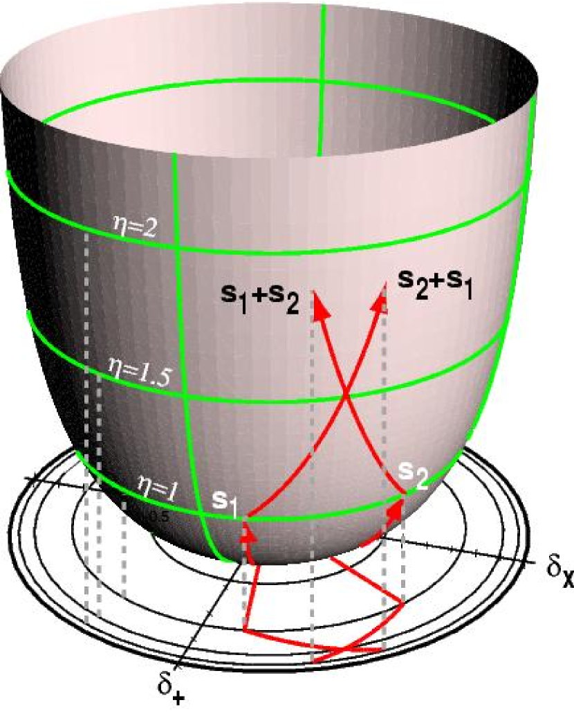
Figure 1: The shaded surface is an embedding of the shear manifold into Euclidean space. The radius vector along this surface is the conformal shear $\eta$; the radius upon projection onto the $xy$ plane is the distortion $\delta$ (or ellipticity $e$). At small $\eta$ the manifold is tangent to the $\delta$  plane, and at large $\eta$ approaches the unit cylinder. Two shear vectors ${\bf s}_{1}$ and ${\bf s}_{2}$ of length $\eta=1$ are plotted from the origin, both on the true shear manifold and in the $\delta$ plane. The result of adding the two vectors is also plotted; displacements do not commute in this non-Euclidean space.

2.4 Definition of Shape

A shear is a transformation of the image plane; we next need a quantity to describe the shape of an arbitrary galaxy image. Let $I$ represent some object whose isophotes are a family of similar ellipses. We can simply parameterize the shape of $I$ by the shear $\eta$ which produces this object from some object $I_{0}$ having circular isophotes, i.e.

$$I_{\mbox{\boldmath$\eta$}}={\bf S}_{\mbox{\boldmath$\eta$}}I_{0}\quad\Rightarrow\quad{\bf S}_{-\mbox{\boldmath$\eta$}}I_{\mbox{\boldmath$\eta$}}=I_{0}.$$ (2-23)

We could thus call $\eta$ the conformal shape of the object, and can think of a given ellipse as a location on the shear manifold. More commonly the distortion is used to define the shape; an object is said to have ellipticity ${\bf e}$ if a shear with distortion $\mbox{\boldmath$\delta$}=-{\bf e}$ makes it circular. We will use the symbol ${\bf e}$ since this quantity agrees with the traditional second-moment definition of ellipticities for truly elliptical objects. Equation (2-23) makes it obvious how an ellipse with shape $\mbox{\boldmath$\eta$}_{1}$ will be transformed under the action of a shear $\mbox{\boldmath$\eta$}_{2}$: we simply add the shear to the shape using the addition rules of shear space [Equation (2-12)]:

$${\bf S}_{\mbox{\boldmath$\eta$}_{2}}I_{\mbox{\boldmath$\eta$}_{1}}=I_{\mbox{\boldmath$\eta$}_{3}},\quad{\rm with}\;\mbox{\boldmath$\eta$}_{3}=\mbox{\boldmath$\eta$}_{2}\oplus\mbox{\boldmath$\eta$}_{1}.$$ (2-24)

Likewise we can also say that a distortion $\delta$ maps the ellipticity ${\bf e}\rightarrow\mbox{\boldmath$\delta$}\oplus{\bf e}.$ In general, an applied shear may be viewed as a shift of all shapes along the shear manifold. We will use ${\bf e}$ to represent the shape of an image, whereas $\delta$ represents a shear, which is a transformation of the image plane. The shape and shear spaces, however, transform identically under an applied shear.

A real galaxy has some image intensity distribution $I({\bf x})$ which may not have elliptical isophotes; we would like to define a shape for an arbitrary image. By analogy to Equation (2-23), all that is needed is some definition of a “round” image. Let ${\bf M}(I)$ be any measurement applied to the image which has the simple property that if ${\bf M}(I)=0$, then $M({\bf S}_{\mbox{\boldmath$\eta$}}I)\neq 0$ for any non-zero shear $\eta$. Then the condition ${\bf M}(I)=0$ is our definition of roundness, and we can assign a unique shape $\eta$ to an arbitrary object $I({\bf x})$ by the condition

$${\bf M}({\bf S}_{-\mbox{\boldmath$\eta$}}I)=0.$$ (2-25)

Any shape defined by such a rule clearly transforms under an applied shear just as an ellipse does, namely via Equation (2-24). With any roundness measure ${\bf M}$ we therefore have a definition of shapes and their mapping under shears that follow the rules of addition in shear space. We do not attempt to prove that the solution to Equation (2-25) exists or is unique.

2.5 Shear in Fourier Space

For consideration of the effects of convolution upon sheared images it will be useful to ponder the action of shears in Fourier space. We first note that shearing an image $I({\bf x})$ by $\eta$ is equivalent to shearing its Fourier transform $\tilde{I}({\bf k})$ by $-\mbox{\boldmath$\eta$}$. For a diagonal shear:

$$\widetilde{{\bf S}_{\mbox{\boldmath$\eta$}}I}(k_{x},k_{y}) = (2\pi)^{-1}\int d^{2}x\,I(e^{-\eta/2}x,e^{\eta/2}y)\exp[2\pi i(k_{x}x+k_{y}y)]$$ (2-26)

$$= (2\pi)^{-1}\int d^{2}x\,I(x,y)\exp[2\pi i(e^{\eta/2}k_{x}x+e^{-\eta/2}k_{y}y)]$$ (2-27)

$$= I(e^{\eta/2}k_{x},e^{-\eta/2}k_{y}).$$ (2-28)

A nondiagonal shear must also satisfy this relation since rotation of the real-space function corresponds to rotation in $k$-space. We can therefore just as easily define a galaxy’s shape by a roundness criterion in $k$-space as in real space. This is useful when considering finite resolution (§6) or when analyzing interferometric images with limited Fourier coverage.

3 Optimal Measurements (without Seeing)

In this section we derive an optimum method of measuring galaxy shapes in the case where the angular resolution and sampling of the instrument are assumed to be perfect. In §6 we will treat the more complex case of seeing-convolved images.

3.1 The Ideal Test for Roundness

We have defined the shape of an image in Equation (2-25) by asking what coordinate shear is needed to make the object appear round. We need to choose a measurement ${\bf M}$ which detects with the highest possible signal-to-noise ratio ($S/N$) any small departure of the image from its round state ${\bf M}=0$. It can be shown that, under some sensible simplifying assumptions about $M$, the solution of Equation (2-25) becomes equivalent to finding the best least-squares fit of an elliptical-isophote model to the galaxy image.

We assume first that the measurement will be a linear function of $I({\bf x})$. Any non-linear method will prove extremely difficult to apply to the case where the image has been convolved with a PSF—it will be hard to use the measurements of bright stars to correct the shapes of faint galaxies for convolution. The most general form of ${\bf M}$ is then

$${\bf M}(I)=\int\!d^{2}\!x\,{\bf W(x)}I({\bf x}),$$ (3-1)

where ${\bf W}$ is some weight function. The weight will be two dimensional, as the measurement must test for departure from roundness in both the $\eta_{+}$ and $\eta_{\times}$ directions in shear space.

We consider first the weight component to detect a small change in $\eta_{+}$. We can decompose the image $I(r,\theta)$ into multipole elements $I_{m}(r)$ via

$$I({\bf x})=I(r,\theta) = \sum_{m=-\infty}^{\infty}I_{m}(r)e^{im\theta}$$ (3-2)

$$I_{m}(r) = \frac{1}{2\pi}\int_{0}^{2\pi}d\theta\,I(r,\theta)e^{-im\theta}$$ (3-3)

We are interested in the change in our measurement upon mapping of the image $I({\bf x})\rightarrow\tilde{I}({\bf x})=I({\bf Sx})$ where ${\bf S}$ is a shear of amplitude $\eta\ll 1$ oriented on the $x$-axis, as in Equation (2-3). The quantity for which we wish to optimize the $S/N$ can thus be written as

$$\delta M=M(\tilde{I})-M(I)=\sum_{m=-\infty}^{\infty}\int_{0}^{\infty}r\,dr\,w_{m}(r)[\tilde{I}_{m}(r)-I_{m}(r)],$$ (3-4)

with $w_{m}$ an arbitrary radial function for each multipole. A little bit of algebra yields the transformation of multipoles

$$\tilde{I}_{m}(r)-I_{m}(r)={\eta\over 4}\left[(m-2)I_{m-2}-rI^{\prime}_{m-2}-(m+2)I_{m+2}-rI^{\prime}_{m+2}\right]+O(\eta^{2}),$$ (3-5)

where the primes denote derivatives with respect to $r$. For an object with truly circular isophotes, we have $I_{m}(r)=0$ for $m\neq 0$, and the only effect of the shear is to induce a quadrupole term $\tilde{I}_{2}=-\eta rI^{\prime}_{0}/4$. For objects without perfect circular symmetry, there are terms beyond the monopole. But for an object to be thought of as “round,” the monopole term $I_{0}$ should dominate the higher multipoles. The monopole is also the only term guaranteed to be positive for all galaxies. Hence the largest effect of the shear will be to alter the $m=\pm 2$ quadrupole intensities (which are conjugates of each other as $I$ is real). The optimal sensitivity to small shear should therefore weight only the quadrupole term:

$$M(I)=\int_{0}^{\infty}r\,dr\,I_{2}(r)r^{2}w(r)={1\over 2\pi}\int\int r\,dr\,d\theta I(r,\theta)w(r)r^{2}e^{-2i\theta}.$$ (3-6)

It is clear that this quadrupole test is the optimal linear measurement for objects with circular symmetry; for more general shapes, the shear has effects on other multipoles that can be measured and used to enhance signal-to-noise (related to the suggestions of Refregier (2001)). But this would require a knowledge of $I_{4}(r)$ and the other multipoles to construct the ideal formula; we settle on the simple quadrupole as the best general solution, as we are always guaranteed that $I_{0}$ is present and positive for any real source. The measurement of some weighted quadrupole is also the normal definition of ellipticity for weak lensing measurements (Miralda-Escudé, 1991).

Combining Equations (3-4), (3-5), and (3-6) we obtain

$$\delta M={-\eta\over 4}\int r\,dr\,r^{2}w(r)[rI^{\prime}_{0}+4I_{4}+rI^{\prime}_{4}].$$ (3-7)

The noise in the measure of $M$ can be derived in two limits: the most common case will be sky-dominated observations, for which the variance of the flux in area $A$ is $nA$, where $n$ is the number of sky photons per unit area (it is assumed that $I$ is in units of photons). In this case we have, from Equation (3-6), the variance of each component of $\delta M$

$${\rm Var}(M)={n\over 4\pi^{2}}\int\int r\,dr\,d\theta r^{4}w^{2}(r)\cos^{2}2\theta.$$ (3-8)

If we ignore the $I_{4}$ terms in Equation (3-7) as being dominated by $I_{0}$ terms, then the choice of weight function which optimizes the detectability of the shear $\eta$ is

$$w_{\rm opt}(r)={-I^{\prime}_{0}\over r}=-{1\over r}{dI_{0}\over dr}.$$ (3-9)

With this optimal weight, the variance of the measurement $M$ would lead to an error in each component of $\eta$ equal to

$$\sigma^{2}_{\eta}={4n\over\pi}\left[\int r^{3}dr\,[I^{\prime}_{0}(r)]^{2}\right]^{-1}.$$ (3-10)

If the object is much brighter than the night sky, then the noise is no longer uniform and the optimization becomes

$${\rm Var}(M) = {1\over 4\pi^{2}}\int\int r\,dr\,d\theta r^{4}w^{2}(r)I(r)\cos^{2}2\theta$$ (3-11)

$$w_{\rm opt}(r) = {-I^{\prime}_{0}\over rI_{0}}=-{1\over r}{d\ln I_{0}\over dr},$$

$$\sigma^{2}_{\eta} = {4\over\pi}\left[\int r^{3}dr\,(I^{\prime}_{0})^{2}/I_{0}\right]^{-1}.$$

3.1.1 Gaussian Objects

An elliptical Gaussian object, when sheared to be circular, will obey

$$I(r,\theta)=I_{0}(r)={f\over{2\pi\sigma^{2}}}e^{-r^{2}/2\sigma^{2}}.$$ (3-12)

In the sky-limited case the optimal weight is the same Gaussian:

$$w_{\rm opt}(r)={-I^{\prime}_{0}\over r}\propto e^{-r^{2}/2\sigma^{2}}.$$ (3-13)

Note that the optimal weight for shape measurement is in this case equal to the optimal filter for detection, i.e. a matched filter. If we define the detection significance $\nu$ as the signal-to-noise ratio for detection of the object with the matched filter, we find

$$\nu^{2} = {{[\int\!d\!A\,w(r)I(r)]^{2}}\over{\int\!d\!A\,nw^{2}(r)}}$$ (3-14)

$$= {{f^{2}}\over{4\pi n\sigma^{2}}};$$ (3-15)

$$\sigma^{2}_{\eta} = {16\pi n\sigma^{2}\over f^{2}}$$ (3-16)

$$= \left({2\over\nu}\right)^{2}.$$ (3-17)

We therefore end up with the simple result that the error in each component of the shear is 2 over the detection significance.

The above derivations assumed that the center and the size $\sigma$ of the Gaussian were known in advance. If there were a sky filled with Gaussian galaxies, we likely would not know in advance the size and location of each. We can determine the centroid in the usual manner by forcing the weighted first moments to vanish:

$$\int\!dA\,wI\,re^{i\theta}=0.$$ (3-18)

The weight for centroiding does not necessarily have to match that used for the shape measurement, but it is convenient to do so. The proper size $\sigma_{w}$ for the weight can be forced to match the size $\sigma$ of the object by requiring the significance to be maximized:

$$0={\partial\nu\over\partial\sigma_{w}}\propto\int\!dA\,wI(1-r^{2}/\sigma_{2}^{2}).$$ (3-19)

In the limit of a Gaussian with low background noise, the Equations (3-11) apply and the optimal weight is uniform. The detection significance in this case is just $\nu=\sqrt{f}$ (with the flux $f$ in photons), and we find again that the standard error in $\eta$ is equal to $2/\nu$. In practice this situation can never be realized because the weight extends to infinity, and at large radii the sky or read noise will dominate the shot noise from the galaxy, and neighboring objects will impinge upon the integrations. We will henceforth confine our discussion to background-limited observations.

3.1.2 Exponential or Other Profiles

To obtain an optimized measurement of a real galaxy we would have to measure its radial profile and construct a custom optimized weight using Equation (3-9). The majority of galaxies are spirals or dwarfs which are typically described by exponential profiles:

$$I(r)\propto e^{-\alpha r}\quad\Rightarrow\quad w_{\rm opt}(r)={e^{-\alpha r}\over r}.$$ (3-20)

This weight diverges at the origin, though all the necessary integrals of the weight are convergent. If the galaxy is truly cusped in the center, then the intensity near the center is very sensitive to small shears and is weighted heavily.

In practice it is simpler to adopt a weight function that is universal (up to a scale factor), especially at low $S/N$ where attempts to measure each individual profile would be pointless. There are a number of reasons to prefer a Gaussian weight:

• The Gaussian drops very quickly at large radii, minimizing interference from neighboring objects. Integrals of all moments are convergent.

• Weights with central divergences or cusps are difficult to use in data with finite sampling, and also amplify the effects of seeing on the galaxy shapes. The Gaussian is flat at $r=0$.

• Gaussian weights are analytically convenient, allowing many useful formulae to be rendered in closed form.

• Gaussian weights allow construction of the family of orthonormal basis functions that we will use in later chapters to compensate measured shapes for finite resolution.

• The Gaussian is not far from optimal for most galaxy shapes. For a well-resolved galaxy with an exponential profile, the Gaussian weight measures $\eta$ with only 7% higher noise than the optimal weight in Equation (3-20). In the presence of seeing, the difference between the Gaussian and optimal weight is even smaller. Recall that any weight we choose yields a valid definition of roundness and hence of shape; the Gaussian just incurs a small penalty in noise level.

The procedure for measuring galaxy shapes is therefore as follows:

1. Estimate a shape $\eta$ for the image $I$ and apply the shear ${\bf S}_{-\mbox{\boldmath$\eta$}}$ to obtain $\tilde{I}$.

2. Iterate the center and size of the Gaussian weight function until the centroid condition (3-18) and the maximum-significance condition (3-19) are satisfied.

3. Compute the second moments with the Gaussian weight function

   $$M(I)=\int\!dA\,w(r)I(r,\theta)r^{2}e^{-2i\theta},\quad w(r)=e^{-r^{2}/\sigma^{2}}.$$ (3-21)

4. If the real and imaginary parts of $M$ are zero, then $\eta$ is the shape of the object. If not, then we use the measured $M$ to generate another guess for $\eta$ and return to step 1.

The process is mathematically equivalent to measuring the second moments of $I({\bf x})$ with an elliptical Gaussian weight, and iterating the weight ellipticity, center, and size until they match the measured object shape. It is therefore an adaptive second-moment measurement. The method is also mathematically equivalent to finding the elliptical Gaussian that provides the best least-squares fit to the image.

3.2 Uncertainties in Shape Estimates

Once we have settled upon a weight of the form $w=e^{-r^{2}/2\sigma^{2}}$, we can integrate $\delta M$ from Equation (3-7) by parts and use (3-8) to calculate the variance in $\eta$. We will again ignore the $I_{4}$ terms; this means we may have a small tendency to over- or under-estimate our shape errors if galaxies tend to be boxy or disky. We first define the weighted flux $f_{w}$, significance $\nu$, and weighted radial moments $\langle Ir^{m}\rangle_{w}$ as

$$f_{w} = \int\!dA\,wI$$ (3-22)

$$\nu^{2}=f^{2}_{w}/{\rm Var}(f_{w}) = f_{w}^{2}/\pi n\sigma^{2}$$ (3-23)

$$\langle Ir^{m}\rangle_{w} = {1\over f_{w}}\int\!dA\,wIr^{m}.$$ (3-24)

The condition (3-19) for optimal significance is

$$\langle Ir^{2}\rangle_{w}=\sigma^{2}$$ (3-25)

and under this condition the variance in each component of the shape is

$$\sigma^{2}_{\eta} = {{4\pi n\sigma^{2}}\over{f_{w}^{2}(1-a_{4})^{2}}}+O(\nu^{-4})$$ (3-26)

$$= {4\over{\nu^{2}(1-a_{4})^{2}}}+O(\nu^{-4})$$ (3-27)

$$a_{4} \equiv {{\langle Ir^{4}\rangle_{w}}\over{2\sigma^{4}}}-1.$$ (3-28)

The quantity $a_{4}$ is a form of kurtosis which is zero for a Gaussian image. The terms of order $\nu^{-4}$ arise from errors in the centroid determination, and are discussed further in §8.

The procedure for measuring an object of shape $\eta$ requires applying a shear $-\mbox{\boldmath$\eta$}$ to the image coordinates ${\bf x}$ to produce a coordinate system ${\bf x^{\prime}}$ in which the object appears round. The uncertainties in Equation (3-26) apply in this sheared coordinate system. Because the object is round in this frame, there is no preferred direction in the shear space and the uncertainty region is circular, with an uncertainty of $\pm\sigma_{\eta}$ on each component $(\eta_{+}^{\prime},\eta_{\times}^{\prime})$ measured in the sheared frame. We must reapply a shear $+\mbox{\boldmath$\eta$}$ to restore our measurement to the original coordinate system. This process is illustrated in Figure 2. The $\eta$ coordinate transformations defined in Equations (2-12), in the limit of $\eta_{1}=\sigma_{\eta}\ll 1$, indicate that the uncertainty region on $\eta$ will be elliptical, with a shrunken principal axis in the circumferential direction of the shear manifold:

$$\sigma_{\theta}={{\sigma_{\eta}}\over{\sinh\eta}}\quad\Rightarrow\quad ds=\tanh\eta\,\sigma_{\theta}=\sigma_{\eta}\,{\rm sech}\,\eta.$$ (3-29)

If we instead use Equations (2-16), we can find the uncertainty ellipse in the ellipticity plane to be

$$\begin{array}[]{rcl}\sigma_{e}&=&(1-e^{2})\sigma_{\eta},\\ e\,\sigma_{\theta}&=&\sqrt{1-e^{2}}\sigma_{\eta}.\end{array}$$ (3-30)

So on the ${\bf e}$ unit circle, the uncertainty ellipse shrinks radially by $1-e^{2}$ and tangentially by $\sqrt{1-e^{2}}$ as we transport the error region from the origin back to the original ellipticity ${\bf e}$.

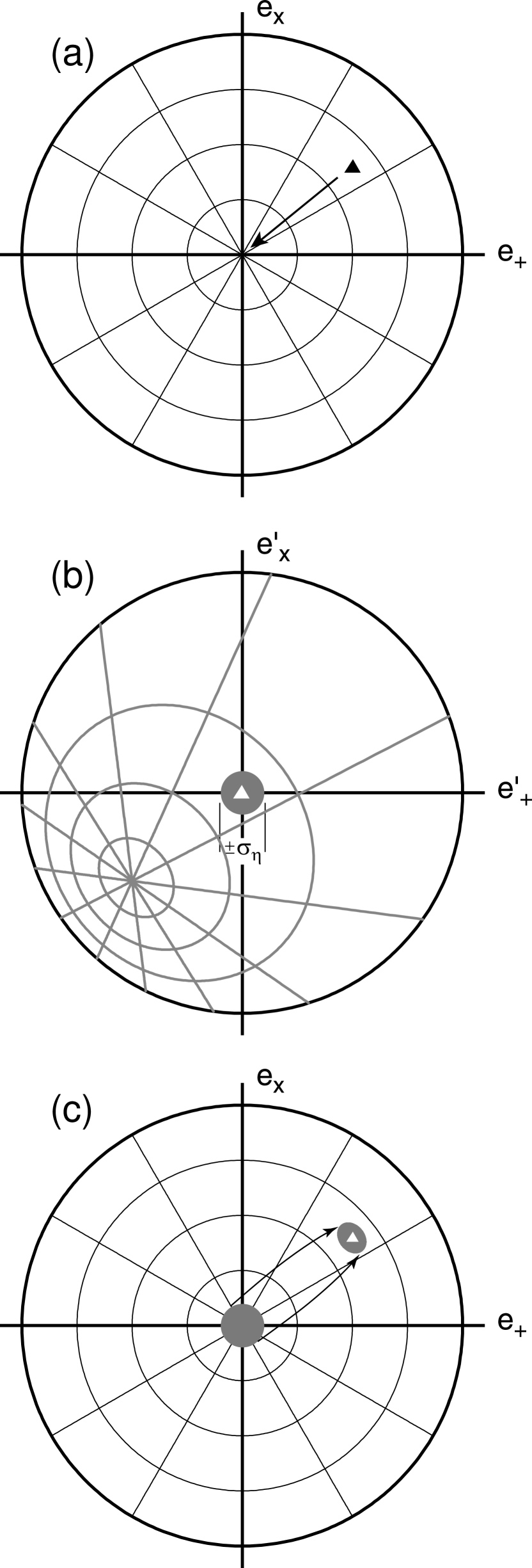
Figure 2: The scheme for ellipticity measurement and its errors are illustrated schematically: in (a), the triangle marks the true shape of a target galaxy, located in the e plane. The shape is determined by shearing the image until the galaxy appears round. In the ellipticity plane, we are moving the object along the vector to the origin. Panel (b) shows the location of the target (and the original coordinate grid) in the e plane after application of the shear that makes it round. The shaded region represents the uncertainty region for the shape in the sheared view—the error region must be circular because the image is round. Finally in (c) we undo the applied shear, shifting the target and the error region back to the original shape. This mapping, however, shrinks the error region by a factor $1-e^{2}$ ($\sqrt{1-e^{2}}$) in the radial (azimuthal) axes.

Note that our derivation assumes that the noise characteristics of the image are unchanged when we apply a shear. This is true in the background-limited case because the noise spectrum is flat, and our shear matrices ${\bf S}$ have unit determinant. For an image that has been smoothed or deconvolved, the power spectrum will have structure and the shear will alter the noise statistics. We will discuss this in §6 in the context of finite image resolution.

3.3 Comparison with Other Methods

Galaxy ellipticities for weak lensing were first determined by computing unweighted second moments of the intensity (Tyson, Valdes, & Wenk, 1990). If the moment integrals are taken to infinity, then the measured ellipticities transform under shear using the addition rules in Equation (2-13), and furthermore the correction for PSF effects is extremely simple. It is clearly impractical, however, to carry the integrals to infinity, since neighboring objects will interfere, the noise is divergent, and, as noted by K00, many common PSFs have divergent second moments. So the initial methods generally used some sort of isophotal cutoff to the moments. This has the disadvantage of creating moments which are non-linear in the object flux. An alternative would be to use unweighted moments within a fixed circular aperture, but as noted by KSB, the noise properties of unweighted moments are far from optimal.

In the KSB method, the measured ellipticity ${\bf\hat{e}}_{\rm KSB}$ is computed from the second moments measured with a circular Gaussian weight with size selected to maximize the detection significance $\nu$. [A different weight function was suggested by Bonnet & Mellier (1995).] The distinction between the KSB method and ours is that KSB always apply a weight which is circular in the original image plane; in our adaptive method, the weight is circular in the sheared image plane which makes the object round. Or, as viewed in the original image coordinates, the weight is an ellipse with shape iterated to match that of the object. This distinction has two consequences: first, our adaptive method yields lower uncertainties for non-circular objects because the weight is a better match to the image. This effect is minor, though, for objects with $e\lesssim 0.5$, and a minority of images are more elliptical then this.

The second, more important advantage over the KSB method is that our definition of shape via Equation (2-25) guarantees that our measured ellipticities ${\bf\hat{e}}$ are transformed by an applied shear via Equations (2-13). The circular-weight ${\bf\hat{e}}_{\rm KSB}$ does not have this property—indeed for an object with elliptical isophotes, ${\bf\hat{e}}_{\rm KSB}$ does not equal the true ellipticity. In the KSB method, it is therefore necessary to calculate a “shear polarizability” for each object, describing the response of ${\bf\hat{e}}_{\rm KSB}$ to a small shear $\delta$; this polarizability depends upon the radial profile and $m=4$ moments of the object. The “polarizability” of our measured ellipticities is just the $\delta\ll 1$ limit of Equations (2-13):

$${\bf e}\rightarrow{{{\bf e}+\mbox{\boldmath$\delta$}}\over{1+\mbox{\boldmath$\delta$}\cdot{\bf e}}}\approx{\bf e}+\mbox{\boldmath$\delta$}-{\bf e}(\mbox{\boldmath$\delta$}\cdot{\bf e}).$$ (3-31)

This transformation rule, and the shapes of our uncertainty regions in ellipticity space, arise solely from the geometry of the shear manifold and are independent of the details of the galaxy images. This will simplify the following discussions of methods to derive a shear from an ensemble of measured galaxy shapes.

We implement the adaptive-weighted-moments scheme in the program ellipto, described further in Jarvis et al. (2002).

4 Combining Exposures

In a typical observing program, a given background galaxy is imaged in a number of different exposures, in one or more bandpasses. This is done to increase exposure time, permit rejection of cosmic rays, and/or gather color information. Multiple exposures can also reduce systematic effects by placing data for a given galaxy on different parts of the detector and in different seeing conditions.

We hence encounter the question of how to combine data on a given galaxy in different images to an optimal single measure of the shape. There are two possible approaches:

1. Measure the shape on each exposure, then create a weighted average of the measurements as the final shape.

2. Register and average the images, then measure the object on the combined image.

We first consider which offers the lowest noise on the final shape. Consider the task of combining $N$ exposures, with the object having significance $\nu_{0}$ on each exposure. Following Equation (3-26), the uncertainty in the shape of a nearly-round object measured from a single image will be

$$\sigma^{2}_{\eta,0}={4\over\nu_{0}^{2}}+C^{\prime}\,[{\rm Var}(x_{0})]^{2}=4\nu_{0}^{-2}+C\nu_{0}^{-4}.$$ (4-1)

The second term is the uncertainty due to centroiding error, and $C$ and $C^{\prime}$ are constants of order unity. If we average measurements (Method 1), then we decrease $\sigma_{\eta}$ by $\sqrt{N}$. If we average images (Method 2), then we increase $\nu$ by $\sqrt{N}$. The net error on the shape in the two cases is then

$$\sigma_{\eta}={2\over{\sqrt{N}\nu_{0}}}\cases{\sqrt{1+C/2\nu_{0}^{2}}&\hbox{Method 1}\cr\sqrt{1+C/2N\nu_{0}^{2}}&\hbox{Method 2}\cr}$$ (4-2)

The two methods are equivalent, except for the centroiding noise. If $\nu_{0}$ is not $\gtrsim 5$ than averaging images will produce better accuracy on $\eta$. Keep in mind that (a) the galaxy will not even be detected on the individual exposures unless $\nu_{0}\gtrsim 3$, and (b) the galaxy is useless for weak lensing unless $\sigma_{\eta}\lesssim 0.5$, which requires $N\nu_{0}^{2}\gtrsim 16$. When $N\lesssim 3$, the centroiding penalty is small for any object that will be useful, so a combined image is extraneous. When $N\gtrsim 5$, there are many galaxies detectable on the summed image that are not detectable on the individual images, and a summed image has detectability and centroid-noise advantages.

There is a compromise, “Method 1.5,” which has the practical advantages (delineated below) of Method 1, while retaining the small $S/N$ edge of Method 2: that is to create a summed image and use it for object detection and centroid determination, so that ${\rm Var}(x_{0})\approx 1/N\nu_{0}^{2}$. Then this centroid is used to measure shapes on individual exposures, and the shape errors are equivalent to Method 2. In practice we will combine deconvolved Laguerre coefficients (§6.3) rather than measured shapes.

There are several reasons why it may be preferable to average catalogs instead of images:

• Correction of shapes for PSF effects is paramount, and only possible if the PSF is constant or slowly varying across the image. If the different exposures in a summed image overlap only partially, then the PSF (and noise level) will jump discontinuously as one crosses the boundaries of component exposures. It is therefore preferable to correct for PSF effects on an exposure-by-exposure basis. If the PSF is very stable (e.g. a space telescope) or if the exposures all have nearly the same pointing (a single deep field), then a summed image will have well-behaved PSF variations.

• For the smallest objects, the exposures with the best seeing will contain nearly all the useful shape information and should be weighted heavily (Kochanski & Fisher, 1994). Large objects are, on the other hand, measured equally well in every exposure. Averaging catalogs allows one to adjust the weights of different exposures on an object-by-object basis, whereas this is not possible when combining images.

• If there are exposures in different bands, then the optimal weighting of the exposures is dependent upon the color of the object. This is easily done when averaging cataloged shapes but not easily done by summing images.

• Creation of a summed image requires registration and interpolation of pixels. The latter process smoothes the noise field and causes subtle variations in the PSF, both of which complicate later analyses.

• An especially pernicious hazard to creating a summed image is that slight mis-registration of the component images will cause coherent elongations of the images, which if not corrected will mimic a lensing signal. This is discussed by KSB; in theory such effects are handled by a proper PSF correction scheme. This is a danger for Method 1.5 as well.

Some practical advantages to Method 2, combining images, are that:

• The data storage and processing requirements can be lower for a single combined image if $N$ is large.

• In Method 1, outliers (from cosmic rays) are rejected on an object-by-object basis, whereas in Method 2 rejection is pixel-by-pixel. If the galaxies are very oversampled and the cosmic-ray rate is high, Method 2 could salvage the un-contaminated parts of galaxy images that Method 1 discards.

For the simplest circumstances (a single-filter stack of images with common pointing), image averaging is easier and has few drawbacks. For multi-filter or mosaicked data, catalog averaging is needed. The hybrid Method 1.5 is best for such cases, though more work. In the rest of this section we detail procedures for each Method.

4.1 Combining Images

There are standard tools for combining exposures into a single image. We remark here upon a few special considerations when doing this for weak lensing observations.

First, accurate registration is paramount. Our scheme for image registration is described in Jarvis et al. (2002).

Second, the use of median algorithms is commonplace but dangerous. Proper correction for PSF effects will require that the images of bright stars have precisely the same PSF as do the faint galaxies. But with a median algorithm, the bright, high-$S/N$ stars will be constructed with a PSF which is a median of all the exposures. The images of faint objects, however, will tend toward a PSF that is the mean of all the exposures, because the noise fluctuations will dominate PSF variations. The final PSF will therefore vary with magnitude. A sigma-clipping average is much preferred over the median for the necessary task of cosmic-ray rejection when combining.

Similarly one must be careful about rejecting saturated pixels. There will be many stars which saturate only on the best-seeing exposures; if the saturated pixels are rejected, these stars will have final PSFs which are broader than the PSF for faint objects. One must take care to ignore stars which are saturated in any one of the exposures.

4.2 Combining Shape Measurements

Suppose that a given galaxy has been measured to have ellipticity ${\bf e}_{i}$ in images $i\in\{1,2,\ldots,N\}$. We desire the ${\bf e}$ which best estimates the true ellipticity of the object. Using the results of §3.2, we see that in the absence of PSF distortions, the minimum-variance estimate of ${\bf e}$ will be that which minimizes the $\chi^{2}$ given by

$$\chi^{2}=\sum_{i}({\bf e}\ominus{\bf e}_{i}){\bf S}_{i}^{-1}({\bf e}\ominus{\bf e}_{i})$$ (4-3)

Here, ${\bf e}\ominus{\bf e}_{i}$ is equivalent to ${\bf e}\oplus(-{\bf e}_{i})$, where $\oplus$ corresponds to the addition operator introduced in Equation (2-11), and ${\bf S}_{i}$ is a covariance matrix which is $\sigma_{\eta}^{2}{\bf I}$ in simple cases.

Note that if the ${\bf e}_{i}$ are measured in different filters, than the galaxy may have no single well-defined ellipticity. By “best estimate,” then, we must mean that which offers the best sensitivity to a weak lensing distortion, and the minimum-variance combination of the ${\bf e}_{i}$ is still the desired quantity.

The $\ominus$ is a non-linear operator, so we could use a non-linear minimization algorithm to find the value of ${\bf e}$ at which $\chi^{2}$ is minimized. However, this is both impractical for time considerations and unnecessary since the values of $\sigma_{\eta}$ are usually small. Thus, we can linearize the subtraction operator

$${\bf e}\ominus{\bf e}_{i}={\bf T}_{i}({\bf e}-{\bf e}_{i})+O(({\bf e}-{\bf e}_{i})^{2})$$ (4-4)

T can be derived from Equations (2-13)

$${\bf T}={1\over{1-e^{2}}}\left[I-{{1-\sqrt{1-e^{2}}}\over{e^{2}}}\left(\begin{array}[]{cc}e_{\times}^{2}&-e_{\times}e_{+}\\ -e_{\times}e_{+}&e_{+}^{2}\end{array}\right)\right]$$ (4-5)

The linearized $\chi^{2}$ becomes

$$\chi^{2} = \sum_{i}({\bf e}-{\bf e}_{i})\mbox{\boldmath$\Sigma$}_{i}({\bf e}-{\bf e}_{i}),$$ (4-6)

$$\mbox{\boldmath$\Sigma$}_{i} \equiv {\bf T}_{i}^{T}{\bf S}_{i}^{-1}{\bf T}_{i}$$ (4-7)

which has a minimum at

$${\bf e} = \left(\sum_{i}\mbox{\boldmath$\Sigma$}_{i}\right)^{-1}\left(\sum_{i}\mbox{\boldmath$\Sigma$}_{i}{\bf e}_{i}\right)$$ (4-8)

$${\rm Cov}({\bf e}) = \left(\sum_{i}\mbox{\boldmath$\Sigma$}_{i}\right)^{-1}$$

This is a standard least-squares solution for the mean of the ${\bf e}_{i}$ given covariances $\mbox{\boldmath$\Sigma$}_{i}$ in a Euclidean ${\bf e}$ space. In the simple case of ${\bf S}=\sigma_{\eta}^{2}{\bf I}$, the expression for $\mbox{\boldmath$\Sigma$}_{i}$ simplifies considerably to

$$\mbox{\boldmath$\Sigma$}={1\over{\sigma_{\eta}^{2}(1-e^{2})^{2}}}\left(\begin{array}[]{cc}1-e_{\times}^{2}&e_{\times}e_{+}\\ e_{\times}e_{+}&1-e_{+}^{2}\end{array}\right),$$ (4-9)

which is equivalent to Equation (3-30). However, when we apply corrections for PSF dilution, we will find that the covariance matrix is more generally an ellipse with axes aligned in the radial and tangential directions. That is,

$$\mbox{\boldmath$\Sigma$}={\bf R}_{\theta}\left(\begin{array}[]{cc}\sigma_{e}^{2}&0\\ 0&e^{2}\sigma_{\theta}^{2}\end{array}\right){\bf R}_{-\theta}$$ (4-10)

where ${\bf R}_{\theta}$ is a rotation matrix with $\theta=\arctan\left({e_{\times}\over e_{+}}\right)$. In either case the minimization (4-8) is numerically straightforward, and we are left with an uncertainty ellipse for the mean ${\bar{e}}$. It is wise to implement some outlier-rejection algorithm in this process as well.

5 Estimating Shear from a Population of Shapes

Now we presume to have measured ellipticities ${\bf e}_{i}$ for a set of $N$ distinct galaxies, with known measurement uncertainties for each. Our final task is to create a statistic $\hat{\mbox{\boldmath$\delta$}}$ from the ${\bf e}_{i}$ which best estimates the lensing distortion $\delta$ that has been applied to this ensemble. There are three main effects which must be considered in constructing the estimator: first, the ${\bf e}_{i}$ respond differently to an applied distortion $\delta$, as embodied by Equation (3-31) for true ellipticities, or by shear polarizabilities for the KSB estimators, so we need to know the responsivity ${\cal R}\equiv\partial\hat{\mbox{\boldmath$\delta$}}/\partial\mbox{\boldmath$\delta$}$ of our statistic. Second, the variety of ellipticities in the parent (unlensed) galaxy population causes shape noise in the shear estimate. In most weak lensing projects this is the dominant random error, and we wish to minimize its effects. Third, there is measurement error in each ellipticity, which we also wish to minimize in our shear estimator.

Most practitioners have adopted a simple arithmetic mean of $e_{+}$ and $e_{\times}$ as estimators for the applied distortion (e.g. Fischer & Tyson 1997). Using the weak-distortion Equations (3-31), it is easy to see that, in the absence of measurement error, this estimator has a responsivity ${\cal R}=1-\sigma^{2}_{\rm SN}$ and a variance ${\rm Var}(\hat{\delta}_{+})=\sigma^{2}_{\rm SN}/N$, where we have defined the shape noise $\sigma^{2}_{\rm SN}\equiv\langle e^{2}_{+}\rangle$ (the $\times$ component has the same properties and shape noise).

Others have realized, however, that rare, highly elliptical galaxies have too much influence on the arithmetic mean and should be deweighted. Cutoffs on $|{\bf e}|$ (Bonnet & Mellier, 1995) or other weighting functions $w(e)$ (Van Waerbeke et al., 2000) have been applied to the ellipticities and tested with simulations, but without any sort of analytic optimization or justification. Lombardi & Bertin (1998) consider the optimization of a general weighted sum of second moments (rather than ellipticities); this unfortunately couples the ellipticity measurement to the distribution of sizes of the galaxies and leads them to consider only weights which are power-law functions of the moments.

Hoekstra et al. (2000) present a weighting scheme which incorporates both measurement error and the shape noise, and K00 gives a detailed discussion of optimal weighting for distortion measurements. Both are similar to our method in many respects, which we comment upon at the end of this section.

5.1 Without Measurement Error

We start with an unlensed background galaxy population with ellipticities distributed within the unit circle according to

$${{dN}\over N}=P({\bf e^{\prime}})d^{2}\!e^{\prime}=P(e^{\prime})e^{\prime}\,de^{\prime}\,d\theta^{\prime}.$$ (5-1)

A fundamental assumption of weak lensing is that the background is isotropic so that the unlensed population can have $P$ depend only upon the amplitude of ${\bf e^{\prime}}$, not its orientation. The effect of a distortion $\delta$ is to map the background population to a new, anisotropic distribution $P_{\mbox{\boldmath$\delta$}}({\bf e})$, as illustrated in Figure 3. We are given a sample of $N$ galaxies from the new distribution, and our task is to estimate the $\delta$ which gave rise to the distribution from the original $P$.

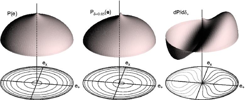
Figure 3: The left panel shows a model for intrinsic distribution $P(e)$ of galaxy shapes over the ${\bf e}$ plane—it must have circular symmetry. When each galaxy is sheared by $\delta_{+}=0.05$, the galaxy distribution shifts to the right as in the middle panel. The right-hand panel shows the change in population under the applied distortion; this is the signal which we wish to detect. Shape noise arises from the Poisson fluctuations in the population, which is proportional to the left-hand panel’s $P(e)$. The optimal weight for $\delta_{+}$ determination is the ratio of the right-hand to the left-hand panel.

One approach is to find the value of $\delta$ which maximizes the likelihood of the observed ${\bf e}_{i}$. This is true when

$$0={\partial\over{\partial\delta_{+}}}\sum\log P_{\mbox{\boldmath$\delta$}}({\bf e}_{i})={\partial\over{\partial\delta_{+}}}\sum\log P(|{-\mbox{\boldmath$\delta$}}\oplus{\bf e}_{i}|).$$ (5-2)

A similar condition holds for $\delta_{\times}$. These equations define the maximum-likelihood $\delta$ even for strong distortions—though there is not in general a closed-form solution for strong $\delta$.

For weak lensing ($\delta\ll 1$), Equation (3-31) and the conservation of number can be used to derive $P_{\mbox{\boldmath$\delta$}}({\bf e})$ to first order in $\delta$.

$$P_{\mbox{\boldmath$\delta$}}({\bf e})\,d^{2}\!e = P(e^{\prime})\,d^{2}\!e^{\prime}$$ (5-3)

$$= P(|{-\mbox{\boldmath$\delta$}}\oplus{\bf e}|)\left|{\partial{\bf e^{\prime}}}\over{\partial{\bf e}}\right|d^{2}\!e$$ (5-4)

$$\approx P\left(e-\mbox{\boldmath$\delta$}\cdot{\bf e}\left({1-e^{2}\over e}\right)\right)\left(1+3\mbox{\boldmath$\delta$}\cdot{\bf e}\right)d^{2}\!e$$ (5-5)

$$P_{\mbox{\boldmath$\delta$}}({\bf e}) = P(e)\left(1+\mbox{\boldmath$\delta$}\cdot{\bf e}\left(3-{1-e^{2}\over e}{d\log P\over de}\right)\right)$$ (5-6)

$$\log P_{\mbox{\boldmath$\delta$}}({\bf e}) = \log P(e)+\mbox{\boldmath$\delta$}\cdot{\bf e}\left(3-{{1-e^{2}}\over e}{{d\log P}\over de}\right)$$ (5-7)

It can further be shown that the maximum-likelihood estimator for $\delta$ takes the form

$$\mbox{\boldmath$\delta$}={1\over N}\sum{\bf e}_{i}\left(3-{{1-e^{2}}\over e}{{d\log P}\over de}\right).$$ (5-8)

The parenthesized expression is thus a weight function for combining ellipticities into a distortion. We can also show that this weight function is optimal in terms of $S/N$ for weak distortions, as follows. Let us create an estimator $\hat{\mbox{\boldmath$\delta$}}$ which is a general weighted sum of the ellipticities,

$$\hat{\mbox{\boldmath$\delta$}}={{\sum w(e_{i}){\bf e}_{i}}\over{\sum w(e_{i})}}={{\int\!d^{2}\!e\,w(e){\bf e}P_{\mbox{\boldmath$\delta$}}({\bf e})}\over{\int\!d^{2}\!e\,w(e)P(e)}}.$$ (5-9)

The response of this statistic to a small applied shear is

$${\cal R}\equiv{{\partial\hat{\delta}_{+}}\over{\partial\delta_{+}}} = {{\sum\left(w^{\prime}{{\partial e}\over{\partial\delta_{+}}}e_{+}+w{{\partial e_{+}}\over{\partial\delta_{+}}}\right)\,\sum w-\sum we_{+}\,\sum w^{\prime}{\partial e\over\partial\delta_{+}}}\over{\left(\sum w\right)^{2}}}$$ (5-10)

$$= {\sum\left[w(1-e^{2}_{+})+w^{\prime}{e_{+}^{2}\over e}(1-e^{2})\right]\over{\sum w}}$$ (5-11)

where in the last line, we have dropped terms linear in $e_{+}$ or $e_{\times}$ which average to zero over an isotropic population. With an isotropic population, the derivative $\partial\hat{\delta}_{\times}/\partial\delta_{\times}={\cal R}$ as well, and the off-diagonal elements of $\partial\hat{\mbox{\boldmath$\delta$}}/\partial\mbox{\boldmath$\delta$}$ are zero.

We may use Equation (5-11) to calculate the response of any weighted estimator by summing over the observed $e_{i}$, because the small difference between observed and intrinsic distributions does not alter ${\cal R}$ to first order. In the case where we have some analytic form for $P(e)$, we may replace the sums with integrals over the distribution to obtain

$$\langle{\cal R}\rangle = {{\int\!d^{2}\!e\,w(e)e_{+}(\partial P_{\mbox{\boldmath$\delta$}}/\partial\delta_{+})}\over{\int\!d^{2}\!e\,w(e)P(e)}}$$ (5-12)

$$= {{\int\!d^{2}\!e\,w(e)e_{+}^{2}P(e)\left(3-{{1-e^{2}}\over e}{{d\log P}\over{de}}\right)}\over{\int\!d^{2}\!e\,w(e)P(e)}}$$ (5-13)

In the absence of measurement noise, the variance in $\hat{\mbox{\boldmath$\delta$}}$ is due to shot noise. Assuming that the background galaxies obey Poisson statistics and their shapes are randomly assigned, we can propagate the Poisson errors through Equation (5-9) to get the expected error

$${\rm Var}(\hat{\delta}_{+}) = {{\int\!d^{2}\!e\,w^{2}(e)e_{+}^{2}P(e)}\over{N[\int\!d^{2}\!e\,w(e)P(e)]^{2}}}$$ (5-14)

$$= {{\sum w^{2}(e)e_{+}^{2}}\over{\left[\sum w(e)\right]^{2}}}.$$ (5-15)

In (5-15) it is assumed that the sum is over a sufficiently large ensemble of background galaxies to sample the distribution $P(e)$. Any weak lensing measurement has thousands of background galaxies, so this gives a direct estimate of the error in the shear.

The optimal weight is that which minimizes ${\rm Var}(\delta_{+})/{\cal R}^{2}$, which is

$$w_{\rm opt}(e) \propto 3-{{1-e^{2}}\over e}{{d\log P}\over{de}}$$ (5-16)

$$= 3+2{{d\log P}\over{d\log(1-e^{2})}}$$ (5-17)

$$\Rightarrow\quad\sigma_{\delta} = \left[N\int\!d^{2}\!e\,P(e)e_{+}^{2}\left(3+2{{d\log P}\over{d\log(1-e^{2})}}\right)^{2}\right]^{-1/2}.$$ (5-18)

where the last line gives the optimized error in $\hat{\delta}_{+}/{\cal R}$, which is our calibrated estimate of the distortion. Equation (5-16) reproduces the maximum-likelihood solution in Equation (5-8). This may be compared to the distortion uncertainty for equal weighting $w=1$,

$$\sigma_{\delta}={1\over\sqrt{N}}\left({{\langle e_{+}^{2}\rangle^{1/2}}\over{1-\langle e_{+}^{2}\rangle}}\right)=\left({{\sigma_{\rm SN}}\over{1-\sigma^{2}_{\rm SN}}}\right).$$ (5-19)

We first see that a simple arithmetic mean of the ellipticities is the optimum estimator only if $P\propto(1-e^{2})^{\alpha}$ for some exponent $\alpha$. For the real galaxy population, there can be a significant gain in accuracy through use of $w_{\rm opt}$ over equal weighting. An extreme case is a population of randomly oriented circular disks, for which

$$P(e) = {1\over{2\pi e}}(1-e)^{-1/2}(1+e)^{-3/2}$$ (5-20)

$$\Rightarrow\quad w_{\rm opt}(e) = {{1+e}\over{e^{2}}}.$$ (5-21)

With $w=1$, we would have $\sigma_{\delta}=0.590/\sqrt{N}$. The optimal weight diverges at $e\rightarrow 0$ to take advantage of the extreme sensitivity of $P(e)$ to distortion near $e=0$. The integral in Equation (5-18) in fact diverges at $e=0$, driving $\sigma_{\delta}$ to zero—which would be a significant improvement over the equal-weighting case! Unfortunately any small measurement error or departures from circularity for the disks will smooth out the central spike in $P(e)$, creating a finite value for $\sigma_{\delta}$.

Figure 4 shows the $P(e)$ measured for well-measured galaxies in the CTIO lensing survey (Jarvis et al., in preparation). These shape histograms are derived from 230,000 galaxies which are well resolved ($R>0.4$, under the definitions in Appendix C) and have errors on the intrinsic ellipticity of $\sigma_{\eta}\lesssim 0.03$—primarily galaxies of magnitude $17<m_{R}<22$. The shape of $P(e)$ is observed to be highly dependent upon the surface brightness (SB) of the galaxies. The low-SB galaxies show the rise at $e>0.8$ expected of a disk population, but there the distribution drops at $e>0.95$ instead of diverging—this reflects the finite thickness of the disks. There is also no pole at $e=0$ for the low-SB galaxies, showing that the disks are not perfectly circular. The high-SB galaxies are presumably early types since there are very few with $e>0.5$. While the value of $P(e=0)$ increases with surface brightness, it always remains finite, but with $dP/de<0$. The ideal weight Equation (5-16) therefore grows as $1/e$ as $e\rightarrow 0$, but the contribution to the $S/N$ does not diverge at zero as for perfect disks. None of the $P(e)$ curves is well fit by a single Gaussian or power law.

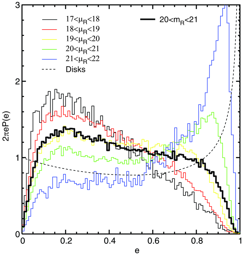
Figure 4: The distribution of intrinsic ellipticities for modestly bright galaxies ($m_{R}\approx 20$) is plotted; we plot $2\pi eP(e)$ rather than $P(e)$ as the nature of the population is more apparent. The distribution is highly dependent upon surface brightness $\mu_{R}$, presumably reflecting the difference between spheroid- and disk-dominated galaxies. The dashed line is the distribution for an isotropic population of circular disks. The high-$\mu$ galaxies are more useful for distortion measurements. The heavy histogram combines all surface brightnesses in the magnitude range $20<m_{R}<21$. Though it is difficult to tell from this plot, $P(e)$ is finite and increasing as $e\rightarrow 0$. Optimal weighting takes advantage of this structure to reduce the noise in the distortion measurement.

The intrinsic ellipticity variance $\sigma_{\rm SN}$ varies from $0.30$ to $0.49$ between the highest and lowest SB bins. The optimally weighted distortion $S/N$ per galaxy for high-SB, early types is 2–3 times higher than for the lowest-SB galaxies, indicating the desirability of incorporating some galaxy-type discriminant—surface brightness, color, or concentration—into the weighting scheme. The only requirement is of course that the discriminant be independent of ellipticity. It seems likely that $P(e)$ will vary substantially with magnitude.

The heavy histogram in Figure 4 combines all well-measured galaxies with $20<m_{R}<21$, which we henceforth use as a representative measure of the real galaxy population. The distribution has $\sigma_{\rm SN}=0.38$, which would lead to $\sigma_{\delta}=0.44/\sqrt{N}$ for an unweighted average. The optimal weighting gives $\sigma_{\delta}=0.33/\sqrt{N}$; the weighting therefore gives a gain equivalent to a 1.8-fold increase in $N$. The gain in telescope time is at least as large. This gain is reduced, however, in the presence of measurement noise, which will tend to wash out the sharp feature in $P(e)$, as discussed next.

We reiterate two favorable results of this section: first, the responsivity ${\cal R}$ and the variance of $\hat{\mbox{\boldmath$\delta$}}$ can be expressed exactly as direct sums over the observed population, for arbitrary choice of $w$; there is no need for calculation of polarizabilities nor recourse to simulated images. Second, we note that the variance in $\hat{\delta}$ can be significantly below the canonical $\sigma^{2}_{SN}/N$ if the ellipticity distribution $P(e)$ has structure that is not washed out by measurement noise.

5.2 With Measurement Error

A galaxy image with true ellipticity ${\bf e}$ will be measured at some ellipticity ${\bf\tilde{e}}$, with a probability distribution of $p({\bf\tilde{e}|e})$. We consider a population of galaxies all having the same significance $\nu$ and resolution parameter $R$ (see §6 and Appendix C), so that they all have a common $p({\bf\tilde{e}|e})$. The measured distribution of ellipticities observed under distortion $\delta$ will then be

$$\tilde{P}_{\mbox{\boldmath$\delta$}}({\bf\tilde{e}})=\int\!d^{2}\!e\,P_{\mbox{\boldmath$\delta$}}({\bf e})p({\bf\tilde{e}|e}),$$ (5-22)

where $P_{\mbox{\boldmath$\delta$}}$ is the distribution of true ellipticities as in the previous section. The symmetry of $P$ and $p$ in the ellipticity plane guarantees that in the absence of distortion, the measured distribution $\tilde{P}(\tilde{e})$ must again depend only upon the magnitude, not the direction, of the measured ellipticity.

Equation (5-22) is not strictly a convolution because the measurement function $p({\bf\tilde{e}|e})$ may depend upon ${\bf e}$ and not simply upon ${(\bf\tilde{e}-e)}$—for example Equation (3-30) describes how the error ellipses contract as ${\bf e}$ departs from zero, even if the significance of the detection is held fixed. In §6 we will show that the behavior of the measurement error is different when the effects of PSF smearing upon the image are important, so at this point we will consider $p({\bf\tilde{e}|e})$ to be, most generally, some kind of Gaussian whose $1\sigma$ ellipse depends only upon the magnitude $e$. An important point is that the functional form of $p({\bf\tilde{e}|e})$ is unchanged by an applied distortion, since $p$ is determined by $\nu$ and $R$, which are unchanged by a pure shear.

Another fact to keep in mind is that, with finite resolution and noise, it is possible to measure $\tilde{e}>1$, if the image noise makes the object appear smaller than the PSF in some dimension. Our formulae should therefore be tractable even for $\tilde{e}>1$, and we cannot simply discard such measurements without contemplating the consequences.

We proceed as in the previous section, by assuming a distortion estimator of the form

$$\hat{\mbox{\boldmath$\delta$}} = {{\sum w(\tilde{e}_{i}){\bf\tilde{e}}_{i}}\over{\sum w(\tilde{e}_{i})}}={{\int\!d^{2}\!\tilde{e}\,w(\tilde{e})\tilde{P}_{\mbox{\boldmath$\delta$}}(\tilde{e}){\bf\tilde{e}}}\over{\int\!d^{2}\!\tilde{e}\,w(\tilde{e})\tilde{P}(\tilde{e})}}$$ (5-23)

$$\Rightarrow\langle{\cal R}\rangle={{\partial\hat{\delta}_{+}}\over{\partial\delta_{+}}} = {{\int\!d^{2}\!\tilde{e}\left[w(\tilde{e})\tilde{e}_{+}\int\!d^{2}\!e\,p({\bf\tilde{e}|e})(\partial P_{\mbox{\boldmath$\delta$}}({\bf e})/\partial\delta_{+})\right]}\over{\int\!d^{2}\!\tilde{e}\,w(\tilde{e})\tilde{P}(\tilde{e})}}$$ (5-24)

$$= {{\int\!d^{2}\!\tilde{e}\left[w(\tilde{e})\tilde{e}_{+}\int\!d^{2}\!e\,P(e)p({\bf\tilde{e}|e})e_{+}\left(3-{{1-e^{2}}\over e}{{d\log P}\over{de}}\right)\right]}\over{\int\!d^{2}\!\tilde{e}\,w(\tilde{e})\tilde{P}(\tilde{e})}}$$ (5-25)

$${\rm Var}(\hat{\delta}_{+}) = {{\int\!d^{2}\!\tilde{e}\,w^{2}(\tilde{e})\tilde{e}_{+}^{2}\tilde{P}(\tilde{e})}\over{N[\int\!d^{2}\!\tilde{e}\,w(\tilde{e})\tilde{P}(\tilde{e})]^{2}}}$$ (5-26)

$$= {{\sum w^{2}(\tilde{e})\tilde{e}_{+}^{2}}\over{\left[\sum w(\tilde{e})\right]^{2}}}.$$ (5-27)

$$\Rightarrow w_{\rm opt}(\tilde{e}) = {1\over\tilde{P}(\tilde{e})}\int\!d^{2}\!e\,P(e)p({\bf\tilde{e}|e}){{e_{+}}\over{\tilde{e}_{+}}}\left(3-{{1-e^{2}}\over e}{{d\log P}\over{de}}\right)$$ (5-28)

Given functional forms for the intrinsic distribution $P(e)$ and the uncertainty function $p$, we could use (5-28) to derive an optimal weight, and use (5-25) and (5-26) to get the responsivity and noise for the estimator using this or any weight function. In most cases these integrals will not have analytic solutions.

The parenthesized quantity under the integral in Equation (5-13) is a galaxy’s responsivity to shear, which depends upon the intrinsic shape. Equation (5-25) is the average of this responsivity for the galaxies with some measured shape. The measurement noise can cause these two quantities to differ; in other words, a naive determination of the responsivity is biased by the measurement noise. KSB-based methods will also suffer a calibration error due to this effect; binning the polarizabilities in parameter space can reduce the noise in the polarizability, but will not remove biases. Precision cosmology will require that such calibration issues be addressed—there are unfortunately no cosmic calibration standards for shear.

The need for $P(e)$ in the above formulae is an unfortunate complication since $\tilde{P}$ is the directly observed quantity. Note that the variance of the estimator can be expressed as a closed sum over the observed shapes (5-27), but the responsivity cannot. A precise calibration of the resultant shear/mass maps requires, therefore, that $P$ be estimated either by deconvolving the observed $\tilde{P}$ with the error distribution $p$, or by recourse to higher-quality images that give $P$ directly.

Derivation of the the optimal weight also requires knowledge of the intrinsic $P$, but we can explore some generic cases, and make some approximations that give workable methods.

5.2.1 Approximate Form For Responsivity with Errors

We wish to have a form for ${\cal R}$ as a sum over the observed objects and applied weights, as in Equation (5-11), for the case of finite measurement errors. Toward that end we can take the derivative of Equation (5-23), which is greatly simplified if we assume that the measurement error, i.e. ${\bf\tilde{e}}_{i}-{\bf e}_{i}$, does not have any first-order dependence on $\delta$. While not strictly valid it is a good approximation. In this case

$${\cal R}={\sum\left[w(1-\langle e^{2}_{+}\rangle_{\tilde{e}})+{\tilde{e}_{+}^{2}\over\tilde{e}}{dw\over d\tilde{e}}\left(1-\langle e^{2}_{+}\rangle_{\tilde{e}}-\langle e_{+}e_{\times}\rangle_{\tilde{e}}\tilde{e}_{\times}/\tilde{e}_{+}\right)\right]\over\sum w},$$ (5-29)

where the brackets indicate an average of the true quantity at a given measured value, e.g.

$$\langle e^{2}_{+}\rangle_{\tilde{e}} = \int d^{2}\!e\,p({\bf e}|{\bf\tilde{e}})e^{2}_{+}$$ (5-30)

$$= {\int d^{2}\!e\,p({\bf\tilde{e}}|{\bf e})P(e)e^{2}_{+}\over\int d^{2}\!e\,p({\bf\tilde{e}}|{\bf e})P(e)}$$ (5-31)

Note that the weight function $w$ may depend upon $\tilde{e}$ directly, but also indirectly through some dependence in its covariance matrix $\Sigma$. If the measurement error function $p({\bf\tilde{e}}|{\bf e})$ and the intrinsic distribution $P(e)$ have circular symmetry, then we must be able to write

$$\langle e^{2}_{+}\rangle_{\tilde{e}}=k_{0}(\tilde{e})+k_{1}(\tilde{e})\tilde{e}^{2}_{+}$$ (5-32)

where $k_{0}$ and $k_{1}$ are functions only of the magnitude, not direction, of ${\bf\tilde{e}}$. We must also have $\langle e_{+}e_{\times}\rangle_{\tilde{e}}=k_{1}(\tilde{e})\tilde{e}_{+}\tilde{e}_{\times}$. Further manipulation, taking advantage of the isotropy of the parent population, yields

$${\cal R}={\sum\left[w\left(1-k_{0}-{k_{1}\tilde{e}^{2}\over 2}\right)+{\tilde{e}\over 2}{dw\over d\tilde{e}}\left(1-k_{0}-k_{1}\tilde{e}^{2}\right)\right]\over\sum w}.$$ (5-33)

This form for ${\cal R}$ depends only upon the observed quantities and the chosen weight scheme, except through the two functions $k_{0}$ and $k_{1}$, which we will approximate below. The resemblance to Equation (5-11) is clear. With this equation and some integration by parts, we may also derive a form for the optimal weighting function:

$$w_{\rm opt}[\tilde{e},\mbox{\boldmath$\Sigma$}(\tilde{e})]=3k_{1}+{1\over\tilde{e}}{dk_{0}\over d\tilde{e}}+\tilde{e}{dk_{1}\over d\tilde{e}}-{1-k_{0}-k_{1}\tilde{e}^{2}\over\tilde{e}}{d\log\tilde{P}\over d\tilde{e}}.$$ (5-34)

5.2.2 Special Case: Gaussians

In general the functions $k_{0}(\tilde{e})$ and $k_{1}(\tilde{e})$ must be calculated numerically using a presumed underlying $P(e)$ for the background population, but analytic solutions are possible in the case of a Gaussian $P(e)$ with variance $\sigma^{2}_{\rm SN}$ in each component (the shape noise) and a constant measurement error $\sigma^{2}_{e}$ on each component. We find that both $k_{0}$ and $k_{1}$ are independent of $\tilde{e}$:

$$\begin{array}[]{rcl}k_{0}&=&(1-f)\sigma^{2}_{\rm SN}\\ k_{1}&=&f^{2}\\ f&\equiv&{\sigma^{2}_{\rm SN}\over\sigma^{2}_{\rm SN}+\sigma^{2}_{e}}.\end{array}$$ (5-35)

The quantity $f$ is the fraction of the total ellipticity variance that is attributable to shape noise. When the measurement noise is small, $f\approx 1$, the ideal weight is close to $(1-\tilde{e}^{2})/(\sigma^{2}_{\rm SN}+\sigma^{2}_{e})$. This is quite similar to the weight adopted by Hoekstra et al. (2000).

For the Gaussian case, $d\log\tilde{P}/d\tilde{e}$ is also quite simple, so Equation (5-33) can be used. In our surveys to date (Smith et al. 2001; Jarvis et al. in prep.) we have adopted a weight that results from optimizing the Gaussian case.

5.2.3 Practical, Nearly Ideal Approximation

We obtain an approximation to the correct responsivity ${\cal R}$ and resultant ideal weight if we adopt the constant $k_{0}$ and $k_{1}$ functions in Equations (5-35) even for non-Gaussian $P(e)$ distributions. The shape noise $\sigma^{2}_{\rm SN}$ may be defined as the assumed variance of the underlying $e_{+}$ and $e_{\times}$, and may be found by subtracting the measurement noise from the observed $\langle\tilde{e}^{2}\rangle$. The measurement noise $\sigma^{2}_{e}$ is known for each galaxy using the methods of this paper; since the covariance matrix for ${\bf\tilde{e}}$ is generally anisotropic, some representative scalar must be selected.

With these guesses for $k_{0}$ and $k_{1}$ in hand, ${\cal R}$ may be estimated with a sum over the observed galaxies using Equation (5-33) for any chosen weight function.

For the real-Universe shape distributions measured in the CTIO survey, we find that the following “easy” weight function offers very close to optimal distortion measurements:

$$w=\left[e^{2}+(1.5\sigma_{\eta})^{2}\right]^{-1/2},$$ (5-36)

where $\sigma_{\eta}$ is the shape uncertainty that the object would have were it circular [cf. Equation (3-30)].

We can check the accuracy of our approximations numerically for chosen $P(e)$ and $p({\bf\tilde{e}}|{\bf e})$ functions. We examine the case when $P(e)$ is that shown in Figure 4 for galaxies with $20<m_{R}<21$, and the measurement error follows Equation (3-30). We find that the weight function given by Equation (5-34) is in fact very close to optimal for all noise levels, even when the simple approximations (5-35) are used for the $k$ functions. The “easy” weight Equation (5-36) also performs nearly optimally, so most applications could use this weight and need not attempt to determine $P(e)$.

A more critical question is whether the approximations (5-35) yield a proper estimate of the calibration factor ${\cal R}$ when used with Equation (5-33). Figure 5 shows how the simple ${\cal R}$ estimator compares to the correct value in Equation (5-25) for our choice of underlying distribution and the “easy” weights (5-36). The approximate form yields a responsivity correct to better than 5% for $\sigma_{\eta}\lesssim 0.4$. It is clear from the Figure that some detailed knowledge of the underlying $P(e)$ distribution will be needed in order to calibrate lensing measurements to the one percent level.

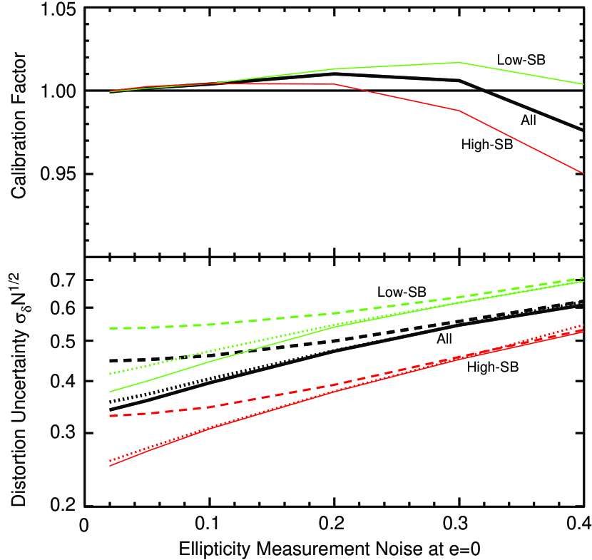
Figure 5: The upper panel plots the approximate, simplified closed-sum estimate of the calibration factor ${\cal R}$ (Equation [5-33]) relative to the exact form (Equation [5-25]), as a function of the ellipticity measurement noise at $e=0$. The weight function is the “easy” Equation (5-36) and the factors $k_{0}$ and $k_{1}$ adopt the simple heuristic approximation (5-35). The heavy (black) curve is for the population of $20<m_{R}<21$ galaxies, the upper (green) curve is for a low-SB sample ($20<\mu_{R}<21$), and the lower (red) curve for a high-SB sample ($17<\mu_{R}<19$), for which the intrinsic $P(e)$ distributions are plotted in Figure 4. The simple formulation yields a calibration accurate to 5% or better in all cases, but 1% accuracy is difficult to achieve. The lower panel shows the uncertainty in the distortion determination when the galaxy shapes are combined with optimum weights (solid lines), the “easy” weights (5-36, dotted), and equal weighting (dashed). The line weights/colors code the galaxy sample, as above. Note that with optimal or easy weighting, the distortion errors continue to shrink even when measurement error is well below the canonical shape noise of $0.3$.

The lower panel of Figure 5 shows the potential advantage of optimal weighting. When the measurement error is $\gtrsim 0.2$, there is little difference between various weighting schemes. For an unweighted distortion estimator, the accuracy levels out as the measurement noise drops below $\sigma_{e}\approx 0.2$. When optimal weights are used, however, the distortion errors continue to drop as the measurement error is pushed toward zero—the optimal weights take advantage of the $e=0$ cusp in the shape distribution. Our “easy” weight scheme recovers nearly all of this potential gain.

To summarize, a practical method of weighting and calibrating the response in the presence of measurement noise is:

1. Determine the underlying $\sigma^{2}_{\rm SN}=\langle e^{2}_{+}\rangle$ of the the intrinsic distribution. The measurement error $\sigma_{\eta}$ (or the full covariance matrix) of each galaxy is known from the formulae in previous sections.

2. Approximate the quantities $k_{0}$ and $k_{1}$ with Equation (5-35).

3. Choose a weight function, for example the “easy” form Equation (5-36), or preferably the optimal form Equation (5-34) which can be derived from the observed distribution $\tilde{P}(\tilde{e})$.

4. The distortion estimator is the sum (5-23). The variance in the estimator is the sum (5-27).

5. The estimator (and variance) must be scaled by the responsivity which is calculated with Equation (5-33).

If more is known about the intrinsic shape distribution, then more accurate functions for $k_{0}$ and $k_{1}$ may be derived and used in the sums.

5.3 Additional Weighting Considerations

The optimal weight may depend upon parameters other than the observed ellipticity $\tilde{e}$. It must, for example, depend upon the measurement errors as described above. If intrinsic shape distribution $P(e)$ depends upon galaxy type, for example, then it may be advantageous to have different weight functions for each type—as long as galaxy type can be determined independent of ${\bf e}$. Ellipticals may be distinguished from spirals, for example, by a concentration ratio such as the $b_{22}$ coefficient described below.

The expected shear will depend upon the redshift $z$ of the background galaxy, and hence there may be a $z$-dependent weight determined from photometric redshift estimates of the background population. More crudely the apparent magnitude may be taken as an indicator of $z$ and used in the weight formulation. The use of such additional weights depends upon the problem being addressed: see Smith et al. (2000) as an example.

5.4 Relation to Previous Methods

The optimal weighting scheme of K00 differs from ours in several respects. It assumes a different measure of ${\bf e}$ which does not follow our geometric transformation relations, so the mean polarizability of galaxies must be calculated in some parameter space, e.g. of flux, size, and $e$. Binning or smoothing in some such space is common to most of the KSB-based weighting schemes as well (Erben et al., 2001; Hoekstra et al., 2000). The variance of the estimators $\hat{\delta}_{i}$ are calculated within each bin, then weights are chosen inversely to the variance of each bin to create a minimum-variance weighted mean estimator. There are three contributors to the variance from each bin:

1. The intrinsic ellipticities of galaxies within the bin are drawn at random from the parent distribution. If $|{\bf e}|$ is one parameter of the space, then only the direction $\theta$ is allowed to vary within the bin. This is of course the shape noise.

2. The measured shape of a given galaxy is drawn from the measurement-error distribution.

3. The number of galaxies within the bin is drawn from a Poisson distribution. If $|{\bf e}|$ is a parameter, then this Poisson noise includes some elements of the shape noise (1) and measurement noise (2).

All three of these effects are important to optimization; all are included in our formulation and (implicitly) in that of K00, so we expect them to be essentially equivalent in the long run—this is not the case, though, for some of the heuristic or parameter-space weight formulations in the literature. The virtue of our scheme is that the nature of the weight function is apparent given the intrinsic shape distribution $P(e)$ and the measurement errors, and there is no need to choose a parameter space for weight selection and polarizability smoothing. Our formulation tells us when further parameters might be desirable, namely when $P(e)$ changes significantly.

6 Measurements with Finite Resolution

The preceding sections outline a method for optimal recovery of weak distortion from galaxy images, and rigorous estimation of the uncertainties on these shears, for the case when the detector views the galaxies with perfect resolution. Unfortunately, the finite resolution of real observations has a strong effect upon shape measurements in every weak lensing observation to date, even those using the Hubble Space Telescope. Finite resolution produces two deleterious effects:

1. A PSF which is not circularly symmetric can induce ellipticities on the images, thus breaking the intrinsic isotropy of the background galaxy population and mimicking a lensing distortion. This is a bias induced by asymmetric PSFs. Since present-day weak lensing surveys are seeking distortion signals well below 1%, measured shapes must be compensated for even the slightest asymmetry in the PSF with some smear correction.

2. Convolution by a circularly symmetric PSF will make most galaxies appear rounder, driving ${\bf e}\rightarrow 0$. This is therefore a dilution of the true lensing signal. While this mechanism cannot create a lensing signal where there is none, it can misleadingly modulate the lensing signal or cause a calibration error in the inferred mass distribution.

Most (but not all) approaches to PSF corrections treat the bias and dilution effects in separate steps. To our knowledge, all published weak-lensing observations have incomplete PSF correction, leaving systematic distortion errors of a fraction of a percent or higher. While in most cases these residual systematic effects have not altered the validity of the authors’ conclusions, the proper correction of PSF effects is presently the largest barrier to the use of weak lensing for precision cosmology.

In §6.1 we review some existing approaches to these problems, in §6.2 we contemplate how one would ideally wish to approach the problem, and in further sections we develop two means of implementing a nearly-ideal approach: one which treats bias and dilution separately, and another which corrects both problems simultaneously with a limited form of deconvolution.

6.1 Existing Approaches to PSF Corrections

6.1.1 The Unweighted Ideal

Unweighted second moments of galaxies are ideal measures of ellipticity—not only do the derived ellipticities transform according to the rules of shear space, but correction for PSF effects is in principle quite simple because the unweighted second moment of the image is just the sum of the original moment and the PSF moment. Thus by subtracting the PSF moments from the measured moments we simultaneously correct for bias and dilution, and obtain the image shape. In the case where the PSF is round, the dilution of a true (pre-seeing) image-plane ellipticity ${\bf e}^{i}$ to an observed (post-seeing) ellipticity ${\bf e}^{o}$ is described by the exact equation

$${\bf e}^{i} = {\bf e}^{o}/R$$ (6-1)

$$R \equiv {{\langle r^{2}\rangle_{i}}\over{\langle r^{2}\rangle_{i}+\langle r^{2}\rangle_{\star}}}$$ (6-2)

$$= 1-{{\langle r^{2}\rangle_{\star}}\over{\langle r^{2}\rangle_{o}}}.$$

The resolution parameter $R$ is determined by the unweighted second radial moment of the measured image $\langle r^{2}\rangle_{o}$ relative to that of the PSF $\langle r^{2}\rangle_{\star}$. Two things to note: first, the error ellipse on the dilution-corrected, pre-seeing ellipticity ${\bf e}^{i}$ is magnified by $1/R$ from the original measurement error Equation (3-30), and is further stretched in the radial direction by the uncertainty in $R$ itself. Thus the error ellipse is no longer simply described by a single $\sigma_{\eta}$. Second, Equation (6-1) can give rise to $|{\bf e}^{i}|>1$, if the noise makes the galaxy look smaller than the PSF about some axis. We cannot arbitrarily discard such measurements without creating a bias in our mean shear. These two phenomena are common to all modes of PSF-dilution correction.

This blissfully simple dilution correction is spoiled by two major problems: first, as discussed above, unweighted second moments have divergent noise properties and for this and other reasons are not practical shape estimators. An equally serious problem noted by K00 is that the second moments themselves are divergent for many realistic PSFs. Further, many galaxies follow deVaucouleurs profiles, for which the second moment converges very slowly.

The simple formulae (6-1) are still valid under the special circumstances that the object and PSF are both Gaussians. The post-PSF object is again a Gaussian, and deconvolution of Gaussians is a simple subtraction of second moments. Hence any shape-measuring algorithm which extracts the proper ellipticity for a Gaussian ellipsoid would allow PSF dilution correction via Equations (6-1) in this limited (and unrealistic) case.

Some early weak lensing measurements (Valdes, Tyson, & Jarvis, 1983) adopt second-moment subtraction as a means of PSF correction, despite the fact that this method is not exact when isophotally-bounded or weighted moments are used, and the images are not Gaussian. This would not suffice, however, for the more sensitive measurements being done today.

6.1.2 Heuristic Methods

In the case of unweighted moments or Gaussians, Equation (6-1) would indicate that a regression of the lensing signal against $\langle r^{2}\rangle_{o}^{-1}$ would yield a distortion free of PSF effects as $\langle r^{2}\rangle_{o}^{-1}\rightarrow 0$. Mould et al. (1994) have attempted to measure very weak shears in the presence of PSF effects using such a regression (though against $\langle r\rangle^{-1}$, in which case a linear relation is not expected). Even with weighted moments, we expect the PSF dilution and bias to decrease as the object becomes well-resolved, so there is some basis to this method, even if it is not exact. Other problems, however, are that the distortion is not likely to be the same for all sizes of galaxy as they likely lie at different distance. Also the regression will lead to substantially higher noise than a more direct dilution correction.

Another approach to the dilution correction is exemplified by FT97, who attempt no analytic correction, instead calibrating the dilution effect by measuring simulated background galaxies which have been subjected to the same distortion, seeing, sampling and noise as the real images. Such a simulation is an essential test of any weak-lensing methodology. The difficulty with sole reliance upon simulated data is that the result is extremely sensitive to one’s ability to exactly match the size-magnitude distribution of the true galaxy population, because the dilution correction is a strong function of size (as in Equation [6-1]) in the typical regime of slightly resolved galaxies. Further, as we show below, the dilution correction depends upon detailed higher-order moments of the galaxy images, which would be very difficult to simulate faithfully. One alternative is to use high-resolution, high-$S/N$ images from HST instead of simulated galaxies—but the total sky area imaged to sufficient $S/N$ by HST is a tiny fraction of a square degree, too small for rigorous calibration tests. It would be preferable to have an analytic correction for dilution, and use the simulated data to spot-check the accuracy of the analytic method.

6.1.3 Perturbative Methods

A step beyond the unweighted-mean approximation to the bias correction is taken by KSB and by FT97. Both make the assumption that the anisotropy of the PSF can be described as a small anisotropic convolution applied to a larger, circularly symmetric PSF. In this case, the effect of the tiny asymmetric deconvolution upon the weighted second moments of a given image can be expressed as a fourth-order weighted moment of the image, which KSB christen the smear polarizability. Given the smear polarizability of an image and a measure of the anisotropy of the PSF, the measured second moments are corrected analytically for the PSF bias.

The FT97 method differs in that the correction for PSF anisotropy is applied to the image rather than to the measured moments: a minimal $3\times 3$ convolution kernel is created which will “circularize” the PSF. The galaxy shapes are measured after this kernel is applied to the image.

The primary drawback to these methods (K00) is that the approximation upon which they are based often fails: a typical diffraction-limited PSF in no way resembles a small convolution to a round PSF, and even a simple aberration such as coma creates PSFs that violate this condition.

These methods have features, however, that we wish to retain in any improved formulation. They are easily adapted to a PSF that varies across the image—the requisite moments of the PSF are measured wherever a star falls upon the image, and interpolated to the location of each galaxy. The FT97 method, by fixing the image, frees us from having to measure the higher-order moments that comprise the smear polarizability, though at the expense of a slight reduction in image resolution and/or an increase in the image noise.

The perturbative methods correct only the PSF bias, not the dilution, because the dilution cannot be considered a small perturbation in any extant data set. FT97 calibrate the dilution with simulations, as mentioned above. The original KSB work made use of empirical calibration as well, as the shear polarizability (cf. §3.3) measures only the susceptibility of the image to a distortion which might be applied after the PSF convolution. Wilson et al. (1996) suggest an empirical calibration by deconvolving the real images, applying a shear, reconvolving, and remeasuring to determine the response. Luppino & Kaiser (1997) introduce the pre-seeing shear polarizability, which approximates the susceptibility of the KSB weighted moments to a shear applied before the PSF. The pre-seeing shear polarizability is, to its lowest order, similar to the resolution factor $R$ introduced above for unweighted moments. There are, however, fourth-order moments of galaxy and stellar shapes involved, and all are measured with Gaussian weights so the noise does not diverge.

The KSB method updated to use the pre-seeing shear polarizability is exact for Gaussians and in the limit of a compact anisotropy kernel, but is not exact in the general case (K00). There are additional ambiguities regarding the appropriate size of the Gaussian weight to be applied when measuring the PSF moments (Hoekstra et al., 1998). The updated KSB method is in wide use, and several papers have investigated how accurately it performs for simulated galaxies and PSFs that are not Gaussian (Erben et al., 2001; Bacon et al., 2000). While it is clear that in many circumstances KSB is good enough, we would prefer to understand and overcome its limitations.

We will demonstrate below that the KSB and FT97 bias corrections are the first terms in a series expansion of the deconvolution of the galaxy image.

Rhodes, Refregier, & Groth (2000) investigate the KSB method in some detail, carrying forth the transformations equations to higher order than do KSB. The PSF corrections, however, still require substantial approximations. Below we construct a hierarchy of all the weighted moments of the image and give general formulae for their transformations under shear, convolution, and other operations.

6.1.4 Deconvolution Methods

Kuijken (1999) suggests that one determine shear by summing the images of all the galaxies in some cell, then comparing this high-$S/N$ summed galaxy image to the PSF. The summed galaxy image should approach circular symmetry in the source plane; the shape of the summed image can thus be modeled relatively simply as a circular source with arbitrary radial profile, sheared by the lens to have elliptical isophotes, then convolved with the PSF. He adopts a flexible parametric representation of this mean radial profile. A candidate profile with candidate lens distortion can be convolved with the known PSF and compared to the measured mean image. The radial profile and distortion are then adjusted to give a best fit. This method can be viewed as a limited form of deconvolution: the only characteristic of the deconvolved image one cares about is the ellipticity; the multipoles beyond quadrupole are irrelevant to the measurement and are discarded.

In Kuijken’s method, the higher-order multipoles are discarded by averaging over many galaxies. This may be difficult in practical situations, where the PSF and/or the distortion signal are varying across the field too rapidly to gather sufficient background galaxies to sum. Another drawback is that summing galaxies’ images may not be the optimal way to combine their information on the shear. Kuijken suggests applying the method to individual galaxies given these potential problems, which amounts to an assumption that the galaxy ellipticity is constant with radius. The accuracy of this method is not discussed in detail. But the method does have the strong advantage of being able to cope with arbitrary PSF behavior, and simultaneously removing both the bias and dilution effects from the measurement.

6.1.5 Commutator Method

K00 introduces a new approach to PSF correction, deriving from the PSF an operator which can be applied to the observed image to effect the transformation of applying a given pre-seeing shear. This operator is derived by considering the commutation of the shear and convolution operators in Fourier space. With the operator in hand, the response to a pre-seeing shear can be determined directly from the post-seeing image, given sufficiently detailed knowledge of the PSF.

The K00 formulation is the first, to our knowledge, to offer an exact correction for PSF bias and dilution. We take a different approach below, and then offer some comparison of the two approaches.

6.2 Optimal Methods in the Presence of a Convolution

In §2.5 we noted that a real-space shear is equivalent to an opposing shear of the Fourier-space image, so that we can conduct the roundness test in Fourier space. One virtue of using a Gaussian weight function for our roundness test, as in Equation (3-21), is that this test takes the exact same form in $k$-space, namely

$$M(I)=0\iff 0=\tilde{M}(\tilde{I})=\int\!d^{2}\!k\,e^{-k^{2}\sigma^{2}/2}I({\bf k})k^{2}e^{-2i\phi}.$$ (6-3)

The only difference is that the Gaussian weight has width $1/\sigma$ in $k$-space, i.e. a broader weight in real space is narrower in Fourier space. Furthermore, our assumed uniform white noise in real space transforms to uniform white noise in Fourier space. Therefore the entire derivation of the optimal weight in §3.1 could have been executed in $k$-space without any change in the result.

The effect of the PSF convolution is to suppress the image by some transfer function $\tilde{T}({\bf k})$. With perfect knowledge of the PSF, we can deconvolve the observed image $\tilde{I}^{o}$ to retrieve the image-plane transform $\tilde{I}^{i}=\tilde{I}^{o}/\tilde{T}$ (here we mean the image plane of the gravitational lens, before the application of seeing). A deconvolution would remove the PSF bias entirely, but the noise is no longer homogeneous in $k$-space, having been amplified (perhaps infinitely) by $1/\tilde{T}$. If the PSF is close to circularly symmetric, then $\tilde{T}$ is nearly independent of direction. If we now imagine making our roundness test on the deconvolved $k$-space image, we adapt Equations (3-7)–(3-9) to give

$$\delta\tilde{M} = {\eta\over 4}\int k\,dk\,k^{2}w(k)k{{d\tilde{I}^{i}_{0}}\over{dk}}$$ (6-4)

$${\rm Var}(M) = {n\over 4\pi^{2}}\int\ k\,dk\,d\phi\,k^{4}w^{2}(k)\cos^{2}2\phi/\tilde{T}^{2}(k).$$ (6-5)

$$\Rightarrow w_{\rm opt}(k) \propto {{-\tilde{T}^{2}(k)}\over{k}}{{d\tilde{I}^{i}_{0}}\over{dk}}.$$ (6-6)

The optimal filter is therefore narrower in $k$-space than both $d\tilde{I}/d(k^{2})$ and $\tilde{T}(k)$. Hence in real space, on the deconvolved image, the optimal filter is broader than both the object and the PSF. This means that we should, sensibly, restrict our roundness test to the region of $k$-space that (a) has signal in the true galaxy image, and (b) is not suppressed below the noise by the convolution.

Our strategy might then be to create some kind of deconvolved image, and apply a Gaussian weight to test for roundness in the deconvolved $k$-space (which is equivalent to using a Gaussian weight in real space). For a Gaussian object with pre-seeing size $\sigma_{i}$ and Gaussian seeing with size $\sigma_{*}$, the optimal weight in deconvolved $k$-space is a Gaussian with size $(2\sigma_{*}^{2}+\sigma_{i}^{2})^{-1/2}$. Such a roundness test is equivalent to a roundness test on the observed, real-space image with a Gaussian weight of size $\sqrt{\sigma_{i}^{2}+\sigma_{*}^{2}}=\sigma_{o}^{2}$. So the optimal size of the weight is again matched to the size of the observed image.

Recall that our algorithm for measuring $\delta$ requires that we shear the coordinates until the object appears round ($\tilde{M}\rightarrow 0$). We want to apply this shear to the deconvolved image. If the object is not round to begin with, then in this sheared coordinate system the transfer function $\tilde{T}({\bf k})$ will no longer have azimuthal symmetry, which will invalidate the above derivation of the optimal weight. We will still have a valid measurement of the shape of the deconvolved object, but possibly with sub-optimal noise level. The increase in noise is a second-order effect, however, so we will not bother to re-optimize the roundness test for this asymmetric noise spectrum.

When the transfer function is anisotropic, then the noise spectrum in the deconvolved image is also anisotropic. There are subtle second-order effects, described in §8, which bias the orientation of the measured shear in the presence of an anisotropy in the noise. Such a noise anisotropy is present after any deconvolution of an anisotropic PSF. A noise anisotropy is also present in the observed image if the PSF is anisotropic and we are not strictly sky-limited. Furthermore, K00 points out a selection bias that can creep into the shear measurements even with a perfectly unbiased shape measurement algorithm. We will discuss means to defeat these biases in §8.

Applying a Gaussian weight in deconvolved $k$-space leads, formally, to divergent noise if $\tilde{T}(k)=0$ for some $k$. This is a real problem, as any finite-sized telescope must produce a transfer function that is identically zero beyond some critical $k_{c}$. The deconvolved image hence has infinite noise for $k>k_{c}$, while the Gaussian weight remains finite. As we shear the $k$-space to make our source appear round, the “wall” of infinite noise moves inwards to $e^{-\eta/2}k_{c}$. In order for our method to remain feasible, our deconvolution algorithm must not attempt to fully deconvolve those portions of $k$-space at or near $k_{c}$, so that the noise remains bounded. There is hence a balance to be struck in executing the deconvolution: we want the carry out the deconvolution to sufficiently high order that the effects of the PSF upon the source ellipticity are removed, but we do not want to deconvolve high-order details that will increase the noise. It would seem, intuitively, that this is possible, since the ellipticity we seek, the Gaussian-weighted quadrupole moment, is a low-order characteristic of the deconvolved image.

The method we describe below is based upon an expansion of the image and PSF into hierarchies of Gaussian-weighted moments—essentially an eigenfunction decomposition. Convolution corresponds to a matrix operation on the vector of moments. The moment vector, and hence the convolution matrix, are formally infinite, but we can choose to truncate the description at some order which we believe to contain all the useful information on the image ellipticity. The convolution matrix is then finite and can be inverted, and the deconvolution executed as a matrix operation. The high-order moments are not deconvolved, so the noise in the deconvolved moments remains finite and in fact close to optimally small. This moment-based method reduces the deconvolution (as well as other transformations) to a matrix multiplication, which can be executed on an exposure-by-exposure basis even for objects with very low $S/N$ on a single exposure, and is therefore very practical for the purpose of weak lensing measurements.

6.3 The Laguerre Expansion

6.3.1 Definitions

The simplicity of the formulae for deconvolution in the special case of Gaussian objects, plus the utility of the Gaussian weight for shape measurements, lead us to seek a description of the image in some Gaussian-based expansion. To maintain the simplest form for convolutions, we look for a decomposition of our images into components which are eigenfunction of the Fourier operator. Such functions will also be eigenfunctions of $(-\nabla^{2}+r^{2})$, hence we are led to the eigenfunctions of the 2d quantum harmonic oscillator (QHO). In one dimension, the QHO eigenfunctions are each a Gaussian times a Hermite polynomial. The Edgeworth expansion, familiar to many astronomers, is a decomposition into 1d QHO eigenfunctions. The 2d version we call the “Laguerre expansion,” using the QHO eigenfunctions

$$I(r,\theta) = \sum_{p,q\geq 0}b_{pq}\psi_{pq}^{\sigma}(r,\theta)$$ (6-7)

$$\psi_{pq}^{\sigma}(r,\theta) = {{(-1)^{q}}\over{\sqrt{\pi}\sigma^{2}}}\sqrt{{q!}\over{p!}}\left({r\over\sigma}\right)^{m}e^{im\theta}e^{-r^{2}/2\sigma^{2}}L_{q}^{(m)}(r^{2}/\sigma^{2})\qquad(p\geq q)$$ (6-8)

$$\psi_{qp}^{\sigma} = \bar{\psi}_{pq}^{\sigma}$$ (6-9)

$$m \equiv p-q.$$ (6-10)

$L_{q}^{(m)}(x)$ are the Laguerre polynomials, which are defined by the generating function (Abramowitz & Stegun, 1965)

$$(1-z)^{-q-1}\exp\left({{xz}\over{z-1}}\right)=\sum_{m=0}^{\infty}L_{m}^{(q)}(x)z^{m}.$$ (6-11)

The Laguerre polynomials satisfy many recurrence relations; the following provide a way to calculate them rapidly:

$$L_{0}^{(m)}(x) = 1$$ (6-12)

$$L_{1}^{(m)}(x) = (m+1)-x$$ (6-13)

$$(q+1)L_{q+1}^{(m)}(x) = [(2q+m+1)-x]L_{q}^{(m)}(x)-(q+m)L_{q-1}^{(m)}(x).$$ (6-14)

A QHO with wavefunction $\psi_{pq}$ has angular momentum $m=p-q$. We will also make use of the quantum number $N=p+q$, which is the excitation energy of the state. Any two of $\{N,m,p,q\}$ suffice to specify the state. The intensity multipole functions $I_{m}(r)$ are composed from the $\psi_{Nm}$ for $N=|m|,|m|+2,|m|+4,\ldots$. The polynomial in $\psi_{pq}$ has terms up to order $N$ in $r$, and $\psi_{pq}$ can also be expressed as the Gaussian times a (complex) polynomial of order $N$ in $x$ and $y$. A few low-order $\psi_{pq}$ are plotted in Figure 6.

Figure 6: The first few of the orthogonal functions $\psi_{pq}$ are plotted. Only the real parts are plotted, with blue (red) for positive (negative) regions. The characteristics are familiar from their use as eigenfunctions of the 2d quantum harmonic oscillator: each has $2m=2|p-q|$ azimuthal nodes and $N-2m$ radial modes, where $N=p+q$ is the number of quanta in the state. The $\psi_{20}$ component is most important as it responds in first order to shear, and hence its absence is our test for “roundness.”

Refregier (2001) has independently introduced the application of QHO eigenfunctions to galaxy shape analysis. Some of the results and ideas presented in this section are presented therein, and applied in Refregier & Bacon (2001), with different notation. Refregier (2001) also presents useful relations for a Cartesian-based family of 2d QHO eigenfunctions. We make use only of the polar family, which are eigenstates of the angular momentum and hence have strong rotational symmetry.

The Laguerre functions have many properties we will find useful. As eigenfunctions of the harmonic oscillator, they are orthonormal, up to the factor $\sigma$ which we introduce in order to give the $b_{pq}$ units of flux:

$$\int\!d^{2}\!x\,\psi_{pq}^{\sigma}({\bf x})\bar{\psi}_{p^{\prime}q^{\prime}}^{\sigma}({\bf x}) = {1\over{\sigma^{2}}}\delta_{pp^{\prime}}\delta_{qq^{\prime}}$$ (6-15)

$$\Rightarrow b_{pq} = \sigma^{2}\int\!d^{2}\!x\,I({\bf x})\bar{\psi}_{pq}^{\sigma}({\bf x}).$$ (6-16)

Thus $b_{pq}$ is a Gaussian-weighted moment of the intensity. Since $I$ is real, we must have $b_{pq}=\bar{b}_{qp}$. When measuring the $b_{pq}$ from an image with uniform white noise, Equation (6-16) yields a covariance matrix for the $b_{pq}$ that is diagonal:

$${\rm Cov}(b_{pq}\bar{b}_{p^{\prime}q^{\prime}})=n\sigma^{2}\delta_{pp^{\prime}}\delta_{qq^{\prime}},$$ (6-17)

where $n$ is the number of counts per unit area. The variance in $b_{pq}$ is shared between the real and imaginary parts, except for $b_{pp}$, which must be real. Non-uniform noise, e.g. shot noise from the galaxy itself, produces a more complicated covariance matrix, as described in Refregier (2001). The significance $\nu$ of detection with the Gaussian filter is given by

$$\nu^{2}={{b_{00}^{2}}\over{n\sigma^{2}}}.$$ (6-18)

Our algorithm for measuring object shapes requires finding the coordinate system in which the centroid is zero (Equation [3-18]) and the roundness test (Equation [3-6]) yields zero. When disregarding seeing, we also set the weight size $\sigma$ by maximizing the significance (Equation [3-19]). These conditions are succinctly stated by the Laguerre coefficients:

Centroid: $$b_{10}=0$$ (6-19)

Roundness: $$b_{20}=0$$ (6-20)

Significance: $$b_{11}=0.$$ (6-21)

The first two of these equations involve both real and complex components, the third is real. We must satisfy these equations by translation, shear, and dilation of the object (or of the underlying coordinate system). These operations can be expressed as transformation matrices acting upon the vector ${\bf b}=\{b_{pq}\}$. The determination of shape is thus efficiently executed by measuring ${\bf b}$ in the original coordinate frame, converting Equation (6-16) to a sum over pixels. Henceforth we can iterate to a solution of our three conditions by manipulating ${\bf b}$, and there is no need to return to the pixel data.

In the case of finite resolution, we wish to satisfy Equations (6-19) and (6-20) for the deconvolved image. We can express the deconvolution as a matrix operation on ${\bf b}$ as well. So we need to find the matrix equivalents of the translation, dilation, shear, and convolution transformations.

6.3.2 Raising and Lowering Operators, Point Transformations

The raising and lowering operators for the 2d harmonic oscillator wavefunctions have the properties:

$$\begin{array}[]{rrcr}a_{p}^{\sigma}={1\over 2}\left[{{x-iy}\over\sigma}+\sigma\left({\partial\over{\partial x}}-i{\partial\over{\partial y}}\right)\right]&a_{p}^{\sigma}\psi_{pq}^{\sigma}&=&\sqrt{p}\,\psi_{(p-1)q}^{\sigma},\\[6.0pt] a_{p}^{\sigma\dagger}={1\over 2}\left[{{x+iy}\over\sigma}-\sigma\left({\partial\over{\partial x}}+i{\partial\over{\partial y}}\right)\right]&a_{p}^{\sigma\dagger}\psi_{pq}^{\sigma}&=&\sqrt{p+1}\,\psi_{(p+1)q}^{\sigma},\\[6.0pt] a_{q}^{\sigma}={1\over 2}\left[{{x+iy}\over\sigma}+\sigma\left({\partial\over{\partial x}}+i{\partial\over{\partial y}}\right)\right]&a_{q}^{\sigma}\psi_{pq}^{\sigma}&=&\sqrt{q}\,\psi_{p(q-1)}^{\sigma},\\[6.0pt] a_{q}^{\sigma\dagger}={1\over 2}\left[{{x-iy}\over\sigma}-\sigma\left({\partial\over{\partial x}}-i{\partial\over{\partial y}}\right)\right]&a_{q}^{\sigma\dagger}\psi_{pq}^{\sigma}&=&\sqrt{q+1}\,\psi_{p(q+1)}^{\sigma}.\end{array}$$ (6-22)

Note that the commutators of the operators are all zero except for $[a_{p},a_{p}^{\dagger}]=[a_{q},a_{q}^{\dagger}]=1$. These operators can be used to formulate the transformation matrices we need. Consider first a dilation of the image $I$ by factor $1+\mu$ with $\mu\ll 1$ to a new image $I^{\prime}$:

$$I^{\prime}(x,y) = I[(1-\mu)x,(1-\mu)y]$$ (6-23)

$$\approx \left\{1-\mu\left(x{\partial\over{\partial x}}+y{\partial\over{\partial y}}\right)\right\}I$$ (6-24)

$$= \left\{1-\mu\left(a_{p}^{\sigma}a_{q}^{\sigma}-a_{p}^{\sigma\dagger}a_{q}^{\sigma\dagger}-1\right)\right\}I$$ (6-25)

$$= \sum b_{pq}\left\{(1+\mu)\psi_{pq}-\mu\sqrt{pq}\,\psi_{(p-1)(q-1)}+\mu\sqrt{(p+1)(q+1}\,\psi_{(p+1)(q+1)}\right\}$$ (6-26)

$$\Rightarrow\quad b^{\prime}_{pq} = (1+\mu)b_{pq}-\mu\sqrt{(p+1)(q+1)}\,b_{(p+1)(q+1)}+\mu\sqrt{pq}\,b_{(p-1)(q-1)}$$ (6-27)

An infinitesimal dilation $\mu$ thus mixes coefficients $(N\pm 2,m)$ into the $(N,m)$ coefficient—as expected, multipole order $m$ is conserved by the transformation. The dilation transformations are thus generated by the matrix

$${\bf d}=1-a_{p}^{\sigma}a_{q}^{\sigma}+a_{p}^{\sigma\dagger}a_{q}^{\sigma\dagger},$$ (6-28)

and the transformation matrix ${\bf D}$ for a finite dilation $e^{\mu}$ can be expressed as

$${\bf D}_{\mu}=\exp[\mu{\bf d}].$$ (6-29)

The finite dilation will preserve $m$ as the generator does, but will mix terms of $N+2j$ together, with $j$ any integer. The matrix elements for the finite dilation are derivable in closed form and in a rapid recursion form; the latter are derived in Appendix A.

The generator s for the shear transformation is also easily expressed in terms of the raising and lowering operators. For a shear $\eta\ll 1$ along the $x$ axis,

$$I^{\prime}(x,y) = I[(1-\eta/2)x,(1+\eta/2)y]$$ (6-30)

$$\approx \left\{1-{\eta\over 2}\left(x{\partial\over{\partial x}}-y{\partial\over{\partial y}}\right)\right\}I$$ (6-31)

$$= (1+\eta{\bf s})I,$$ (6-32)

$${\bf s} = {1\over 4}\left[(a_{p}^{\dagger})^{2}+(a_{q}^{\dagger})^{2}-a_{p}^{2}-a_{q}^{2}\right]$$ (6-33)

$$\Rightarrow\quad b^{\prime}_{pq} = b_{pq}+{\eta\over 4}\left(\sqrt{p(p-1)}\,e^{-2i\beta}b_{(p-2)q}+\sqrt{q(q-1)}\,e^{2i\beta}b_{p(q-2)}\right.$$ (6-34)

$$\left.-\sqrt{(p+1)(p+2)}\,e^{2i\beta}b_{(p+2)q}-\sqrt{(q+1)(q+2)}\,e^{-2i\beta}b_{p(q+2)}\right),$$

$${\bf S}_{\eta} = \exp[\eta{\bf s}].$$ (6-35)

In (6-34) we have inserted the phase factors which result from a shear at arbitrary position angle $\beta$. To leading order, the shear mixes in states with $p$ or $q$ changed by $\pm 2$; in the finite case, the shear transformation mixes together $b_{pq}$ for which $p$ and $q$ each change by any even number. Note that this equation generalizes the weighted-moment transformations in Rhodes, Refregier, & Groth (2000) to all orders. Note also that the KSB method identifies the quantity $b_{20}/b_{00}$ as the ellipticity, so the “shear polarizability” is compactly expressed using Equation (6-34) with $p=2$, $q=0$.

An infinitesimal translation of the image by $(x_{0},y_{0})$ gives

$$I^{\prime}(x,y) = I(x-x_{0},y-y_{0})$$ (6-36)

$$\approx \left(1-x_{0}{\partial\over{\partial x}}-y_{0}{\partial\over{\partial y}}\right)I$$ (6-37)

$$= (1+z{\bf t}-\bar{z}{\bf t}^{\dagger})I,$$ (6-38)

$$z \equiv {{x_{0}+iy_{0}}\over\sigma},$$ (6-39)

$${\bf t} = {1\over 2}\left(a_{q}^{\dagger}-a_{p}\right),$$ (6-40)

$$\Rightarrow\quad b^{\prime}_{pq} = b_{pq}+{z\over 2}\left(\sqrt{q}\,b_{p(q-1)}-\sqrt{p+1}\,b_{(p+1)q}\right)+{\bar{z}\over 2}\left(\sqrt{p}\,b_{(p-1)q}-\sqrt{q+1}\,b_{p(q+1)}\right)$$ (6-41)

$${\bf T}_{z} = \exp[z{\bf t}-\bar{z}{\bf t}^{\dagger}]$$ (6-42)

To leading order the translation changes $p$ or $q$ by $\pm 1$, and the finite translation ${\bf T}_{\bf z}$ mixes all the states together. Appendix A gives the matrix elements for all the finite transformations.

The “smear polarizability” coefficients of KSB could be quickly derived at this point by noting that an infinitesimal convolution along the $x$ direction can be expressed as an average of two images translated by $\pm x_{0}$, which will lead to a smear generator that is second order in the raising and lowering operators. Appendix C gives a closely related derivation.

6.3.3 Shape Measurement from Laguerre Decomposition

Our algorithm for shape measurements (with perfect resolution) is to find the translation z, dilation $\mu$, and shear $\eta$ which must be applied to the image to satisfy the conditions (6-19)–(6-21). If ${\bf b}$ is the vector of Laguerre coefficients for the image $I$, we can write

$${\bf b}^{\prime}={\bf M}\cdot{\bf b}=({\bf S}_{\mbox{\boldmath$\eta$}}{\bf D}_{\mu}{\bf T}_{z})\cdot{\bf b},$$ (6-43)

and the elements of ${\bf b}^{\prime}$ with (pq) = (10), (11), and (20) must vanish. This is in general a complex non-linear equation, but for $\mu,\eta,z\ll 1$ the linearized Equations (6-27), (6-34), and (6-41) yield

$$b^{\prime}_{10} = b_{10}+(b_{10}-\sqrt{2}b_{21})\mu-\text@frac{\sqrt{2}}{4}b_{12}\bar{\eta}-\text@frac{\sqrt{6}}{4}b_{30}\eta$$ (6-44)

$$\qquad-\text@frac{\sqrt{2}}{2}b_{20}z+\text@frac{1}{2}(b_{00}-b_{11})\bar{z}$$

$$b^{\prime}_{11} = b_{11}+(b_{00}+b_{11}-2b_{22})\mu-\text@frac{\sqrt{6}}{4}b_{13}\bar{\eta}-\text@frac{\sqrt{6}}{4}b_{31}\eta$$ (6-45)

$$\qquad+\text@frac{1}{2}(b_{10}-\sqrt{2}b_{21})z+\text@frac{1}{2}(b_{01}-\sqrt{2}b_{12})\bar{z}$$

$$b^{\prime}_{20} = b_{20}+(b_{20}-\sqrt{3}b_{31})\mu+\text@frac{\sqrt{2}}{4}(b_{00}-b_{22})\bar{\eta}-\text@frac{\sqrt{3}}{2}b_{40}\eta$$ (6-46)

$$\qquad-\text@frac{\sqrt{3}}{2}b_{30}z+\text@frac{1}{2}(\sqrt{2}b_{10}-b_{21})\bar{z},$$

writing $\eta=\eta_{+}+i\eta_{\times}$. These linear equations may be solved explicitly for the desired transformation coefficients $\eta$, $\mu$, and $z$. The solution appears much simpler if the object is nearly round, such that $b_{pq}\ll b_{00}$ for $p\neq q$. In this case the transformation parameters are, to leading order,

$$\eta = {{-2\sqrt{2}b_{02}}\over{b_{00}-b_{22}}}$$ (6-47)

$$z = {{-2b_{01}}\over{b_{00}-b_{11}}}$$ (6-48)

$$\mu = {{-b_{11}}\over{b_{00}-2b_{22}}}.$$ (6-49)

From these equations it is clear that $b_{20}$, $b_{10}$, and $b_{11}$ are the primary carriers of information on shape, centroid, and size, respectively. Since the shape component $\eta_{+}$ is $(\eta+\bar{\eta})/2$, its uncertainty is to leading order

$$\sigma^{2}_{\eta}\equiv{\rm Var}(\eta_{+}) = {{2\left[{\rm Var}(b_{20})+{\rm Cov}(b_{20}b_{02})+{\rm Var}(b_{02})\right]}\over(b_{00}-b_{22})^{2}}$$ (6-50)

$$= {{4n\sigma^{2}}\over{b_{00}^{2}}}\left[1-b_{22}/b_{00}\right]^{-2}$$ (6-51)

$$\Rightarrow\quad\sigma_{\eta} = {2\over\nu}\left[1-b_{22}/b_{00}\right]^{-1}.$$ (6-52)

Here we have made use of Equation (6-17) for the covariance matrix in the case of white noise, and Equation (6-18) for the definition of the significance $\nu$. We see that the Laguerre expansion easily reproduces the earlier result in Equation (3-26), with the $a_{4}$ parameter in that equation being simply the strength of the $b_{22}$ coefficient.

With a more tedious procedure we may derive the solution for $\eta$ to second order in $b_{pq}/b_{00}$. We take $b_{pp}\ll b_{00}$ for $p>0$ this time in order to simplify the expression:

$$\begin{array}[]{rl}\displaystyle\eta\approx&-2\sqrt{2}{b_{02}\over{b_{00}-b_{22}}}-2\sqrt{3}{b_{20}b_{04}\over b_{00}^{2}}\\[4.0pt] &\quad+{2b_{01}^{2}-2\sqrt{6}b_{10}b_{03}-2\sqrt{2}b_{01}b_{12}\over b_{00}^{2}}\\[4.0pt] &\quad-2\sqrt{6}{b_{11}b_{31}\over b_{00}^{2}}\end{array}$$ (6-53)

The terms in the first line arise from solving for $\eta=0$; the terms in the second and third lines arise when simultaneously solving the centroid and size constraints, respectively. From these terms one can derive the $O(\nu^{-4})$ terms in the shape uncertainty if desired. But more importantly, this expression uncovers a very significant source of bias in shape measurements: the presence of the $b_{pq}$ in second order means that it is possible for noise to be rectified in the determination of ${\bf e}$. If the noise is anisotropic—as is the case after correction for an anisotropic PSF—then ${\bf e}$ will be biased. We will explore this in more detail in §8.

6.3.4 Fourier Transforms and Convolution

The observed galaxy intensity $I^{o}({\bf x})$ is the convolution of the image-plane intensity $I^{i}({\bf x})$ and the stellar PSF $I^{\star}({\bf x})$:

$$I^{o}({\bf x})=I^{i}({\bf x})\circ I^{\star}({\bf x})=\int\!d^{2}\!{x^{\prime}}\,I^{i}({\bf x^{\prime}})I^{\star}({\bf x-x^{\prime}}).$$ (6-54)

The post-seeing, pre-seeing, and stellar images can be expressed as vectors ${\bf b}^{o}$, ${\bf b}^{i}$, and ${\bf b}^{\star}$, respectively, of coefficients over our eigenfunction sets $\psi_{pq}^{\sigma_{o}}$, $\psi_{pq}^{\sigma_{i}}$, and $\psi_{pq}^{\sigma_{\star}}$. The convolution can then be expressed as a matrix relation

$${\bf b}^{o} = {\bf C}({\bf b}^{\star})\cdot{\bf b}^{i}$$ (6-55)

$$b^{o}_{p_{o}q_{o}} = \sum C^{p_{i}q_{i}p_{\star}q_{\star}}_{p_{o}q_{o}}b^{i}_{p_{i}q_{i}}b^{\star}_{p_{\star}q_{\star}}.$$ (6-56)

We will effect the deconvolution by inverting a truncated version of the matrix ${\bf C}$. Its coefficients are determined by the relation

$$\psi_{p_{i}q_{i}}^{\sigma_{i}}\circ\psi_{p_{\star}q_{\star}}^{\sigma_{\star}}=\sum C^{p_{i}q_{i}p_{\star}q_{\star}}_{p_{o}q_{o}}\psi_{p_{o}q_{o}}^{\sigma_{o}}.$$ (6-57)

The convolution is more easily expressed in $k$-space. With the usual definitions (denoted as “System 3” by Bracewell (1978))

$$\tilde{I}({\bf k}) = (2\pi)^{-1}\int\!d^{2}\!x\,I({\bf x})e^{-i{\bf k\cdot x}},$$ (6-58)

$$I({\bf x}) = (2\pi)^{-1}\int\!d^{2}\!k\,\tilde{I}({\bf k})e^{i{\bf k\cdot x}},$$

the convolution becomes a multiplication, and the matrix coefficients in Equation (6-57) can also be expressed as

$$2\pi\tilde{\psi}_{p_{i}q_{i}}^{\sigma_{i}}\tilde{\psi}_{p_{\star}q_{\star}}^{\sigma_{\star}}=\sum C^{p_{i}q_{i}p_{\star}q_{\star}}_{p_{o}q_{o}}\tilde{\psi}_{p_{o}q_{o}}^{\sigma_{o}}.$$ (6-59)

We now make use of another remarkable property of the Laguerre-exponential eigenfunctions, which is that they are their own Fourier transforms. First we note that $\psi_{00}^{\sigma}$ is a two-dimensional Gaussian, and the transform (6-58) is easily executed to yield a new Gaussian,

$$\tilde{\psi}_{00}^{\sigma}={1\over{\sqrt{\pi}}}e^{-k^{2}\sigma^{2}/2}.$$ (6-60)

The functional form of $\tilde{\psi}_{00}(k)$ matches that of $\psi_{00}(x)$, except that we must send $\sigma\rightarrow 1/\sigma$. Next we can use the definition of the raising operators (Equation [6-22]) to note that

$$\widetilde{a_{p}^{\sigma\dagger}\psi}={{-i}\over 2}\left[\sigma({k_{x}+ik_{y}})-{1\over\sigma}\left({\partial\over{\partial k_{x}}}+i{\partial\over{\partial k_{y}}}\right)\right]\tilde{\psi}\equiv\tilde{a}_{p}^{\sigma\dagger}\tilde{\psi}$$ (6-61)

Thus the $k$-space raising operator has the same form as the $x$-space raising operator, save the $\sigma\rightarrow 1/\sigma$ transformation and an additional factor of $-i$. The same is true of $a_{q}^{\dagger}$. Since $\psi_{00}$ and the raising operators are each unchanged by the Fourier transform, it must be true that all the $\psi_{pq}$ are their own Fourier transforms as well, with appropriate scaling factors of $i$ and $\sigma$. More precisely, we have (cf. [6-8])

$$\tilde{\psi}_{pq}^{\sigma}(k,\phi)={{(-i)^{m}}\over{\sqrt{\pi}}}\sqrt{{q!}\over{p!}}\left(k\sigma\right)^{m}e^{im\phi}e^{-k^{2}\sigma^{2}/2}L_{q}^{(m)}(k^{2}\sigma^{2})\qquad(p\geq q)$$ (6-62)

So the problem of convolving two of our eigenfunctions is reduced to the simpler problem of multiplying the same two eigenfunctions. We may reach several conclusions immediately:

• The convolution of $\psi^{\sigma_{i}}_{N_{i}m_{i}}$ with $\psi^{\sigma_{\star}}_{N_{\star}m_{\star}}$ will produce an observed image with azimuthal order $m_{o}=m_{i}+m_{\star}$. Furthermore the multipole phase of the observed image must be the sum of the phases for the original and PSF images’ coefficients.

• If we choose the scale size $\sigma_{o}$ for the observed image eigenfunctions such that

  $$\sigma_{o}^{2}=\sigma_{i}^{2}+\sigma_{\star}^{2},$$ (6-63)

  then the convolution contains components $\psi^{\sigma_{o}}_{N_{o}m_{o}}$ only for $N_{o}\leq N_{i}+N_{\star}$. Recall also that we must have $N_{o}\geq m_{o}=m_{i}+m_{\star}$, so it must be true that $\psi^{\sigma_{i}}_{p_{i}q}\circ\psi^{\sigma_{\star}}_{p_{\star}q}\propto\psi^{\sigma_{o}}_{(p_{i}+p_{\star})q}$ for $q=0$.

In Appendix B we give a recursion relation to calculate any of the elements $C^{p_{i}q_{i}p_{\star}q_{\star}}_{p_{o}q_{o}}$ that we need to calculate the convolution, and thus the deconvolution.

6.3.5 Deconvolution, Noise Amplification, and Truncation

With the formulae for the convolution matrix ${\bf C}$ in hand, we can investigate the nature of the trade-off between the fidelity of the deconvolution—i.e. the extent to which effects of the PSF upon the shape are removed—and the noise level of the deconvolution. We must truncate the ${\bf b}$ vectors at some finite order $N$ to implement the deconvolution; higher $N$ will remove more of the PSF effects, but also increase the noise level. We can illustrate this phenomenon by considering the simplest case of convolution by a unit Gaussian PSF, $b^{\star}_{pq}=2\sqrt{\pi}\delta_{p0}\delta_{q0}$. Since the PSF has only $m_{\star}=0$ terms, we will have $m_{o}=m_{i}$, so the convolution matrix is block-diagonal and we may deconvolve each $m$ independently. If we choose $\sigma_{o}^{2}=\sigma_{i}^{2}+\sigma_{\star}^{2}$, then the convolution matrix coefficients are zero for $N_{o}>N_{i}$, and hence each block matrix is also upper-triangular. This makes the inversion easy. Using the results of Appendix B, defining a deconvolution parameter $D=\sigma_{i}^{2}/\sigma_{o}^{2}=1-\sigma_{\star}^{2}/\sigma_{o}^{2}$, and using Equation (6-17) for the covariance of the measured moments, the deconvolved value of $b^{i}_{00}$ and its variance are

$$b^{i}_{00} = \sum_{p=0}^{\infty}\left({{1-D}\over D}\right)^{p}(-1)^{p}b^{o}_{pp}$$ (6-64)

$$\Rightarrow\quad{\rm Var}(b^{i}_{00}) = n\sigma_{o}^{2}\sum_{p=0}^{\infty}\left({{1-D}\over D}\right)^{2p}=n\sigma_{i}^{2}{D^{2}\over{2D-1}}\qquad(D>1/2).$$ (6-65)

In practice we could not measure the $b^{o}_{pp}$ to infinite $p$ and we must truncate the sum (6-64) at some finite $p$. The more terms we include, the more accurately we describe the deconvolved $b^{i}_{00}$, but each additional term in the deconvolution adds more noise. For $D>1/2$, the added noise in successive terms drops as $p$ increases, and we could in principle do a complete deconvolution of $b^{i}_{00}$ with finite variance. For $D\leq 1/2$, however, the noise in the deconvolved moment diverges for $p\rightarrow\infty$, and we are forced to truncate the deconvolution matrix.

For ellipticity measurements we are primarily interested in the $b^{i}_{20}$ moment. For this case of a Gaussian PSF, the general $b^{i}_{m0}$ moment deconvolution is

$$b^{i}_{m0} = \sum_{q=0}^{\infty}{1\over D^{m/2}}\left({{1-D}\over D}\right)^{q}(-1)^{q}\sqrt{{q+m}\choose m}b^{o}_{(q+m)q}$$ (6-66)

$$\Rightarrow\quad{\rm Var}(b^{i}_{m0}) = {{n\sigma_{o}^{2}}\over{D^{m}}}\sum_{q=0}^{\infty}\left({{1-D}\over D}\right)^{2q}{{q+m}\choose m}$$ (6-67)

$$= n\sigma_{i}^{2}D\left({D\over{2D-1}}\right)^{m+1}\qquad(D>1/2).$$ (6-68)

We note that these moments also demonstrate the properties that they are noisier than the observed moments, and infinitely so if $D<1/2$ and the deconvolution is not truncated. The noise increases as $m$ increases, as we would expect, since higher spatial frequencies must be recovered.

For a purely Gaussian PSF with $D>1/2$, it is possible to complete the deconvolution with finite noise. A real PSF must have components beyond $b^{\star}_{00}$, since the transfer function vanishes above a critical $k$ value. When we invert the convolution matrix for such a PSF we will find that the variance series akin to (6-65) would diverge for any $D<1$. The best truncation value for the matrix will depend upon the form of the PSF and the accuracy to which we demand correction of PSF effects. We will examine some specific cases in Jarvis et al. (2002).

6.3.6 Analytic or Kernel Correction for PSF Bias?

There are two general means of eliminating the shape bias induced by the PSF. One alternative is to measure the anisotropy of the PSF carefully and apply analytic corrections to the measured objects, as occurs naturally within the deconvolution framework described in the preceding paragraphs. The KSB formalism contains an approximate analytic correction. The other method is to convolve the image with a spatially-varying kernel which removes the anisotropy from the PSF, as first demonstrated by Fischer & Tyson (1997) and further advocated in K00. Removal of the PSF bias is the most critical task for a weak lensing method: the PSF dilution is only a calibration error or signal modulation, but the PSF bias introduces a first-order false signal to the lensing analysis.

Ideally, analytic correction is preferred. The convolution kernel will always degrade the image resolution to some extent. Many PSFs cannot be “rounded out” unless the kernel is of size comparable to the PSF itself (K00). Furthermore the convolution will perturb the noise spectrum of the image, complicating error estimation. The kernel method, however, can for simple kernels be faster than an involved analytic correction, especially if eliminating the bias is more important than calibrating the dilution for the task at hand.

The kernel method may offer peace of mind. The demands for rejection of the PSF bias are very stringent: PSF ellipticities of 10% are not uncommon, yet state-of-the-art lensing surveys require systematic errors below 0.1%, so the method we choose must reduce the PSF bias by over 2 orders of magnitude. If the kernel method can make the PSF truly round, then symmetry principles preclude any artificial coherent ellipticity. We flesh out this statement in §7. We may have more trust in the symmetry principle than we do in an analytic correction, especially when finite sampling is taken into account. Note, however, that the symmetry principle requires that the noise power spectrum is also isotropic; §8 below demonstrates how anisotropic noise can bias shape measurements through centroid bias.

We therefore will describe an alternative procedure: eliminate the bias with a kernel correction; measure the shapes, either isotropizing the noise or making a correction for centroid bias; then correct them for dilution with a heuristic formula such as Equation (6-1). In §7 we describe a rounding-kernel methodology, and in Appendix C we derive a higher-order version of the dilution correction. These methods were used by Fischer et al. (2000), Smith et al. (2000), and the forthcoming CTIO lens survey.

6.4 Pixellated Data

Real astronomical data is integrated into pixels and sampled at finite intervals, and the continuum limit that we have assumed in our analysis is not strictly valid. A formal description of the process is that the PSF is altered by convolution with the pixel response function (PRF) to produce the effective PSF (ePSF), which is then sampled at the pixel pitch $a$—see Lauer (1999) or Bernstein (2001) for further elaboration. If the pixel pitch is coarser than the Nyquist interval of the PSF ($\lambda/2D$ for a diffraction-limited image), then there is aliasing and we cannot unambiguously reconstruct the original image or the true $b_{pq}$ coefficients.

In the case where the pixel size $a$ is small compared to the PSF size, the $b_{pq}$ may be estimated by converting the integral Equation (6-16) into a sum over pixels. But the formally correct procedure is to fit the vector of sampled pixel fluxes $I_{i}$ with a model galaxy with free $b^{o}_{pq}$. This is a standard minimization problem for the $\chi^{2}$ parameter

$$\chi^{2}=\sum_{i}{\left(I_{i}-\sum_{pq}b^{o}_{pq}\psi^{\sigma}_{pq}({\bf x}_{i})\right)^{2}\over{\rm Var}(I_{i})}.$$ (6-69)

Since the model is linear, the solution for $b^{o}_{pq}$ and its covariance matrix have a closed form, but of course the number of $b^{o}_{pq}$ coefficients allowed in the model must be less than the number of pixels being fit. With the best-fit coefficients and their covariance matrix in hand, we may proceed with the methods outlined above. It is the ePSF rather than the PSF that has convolved the source image, but since we in fact measure the ePSF for stars, the deconvolution procedures are unchanged. Dithered exposures can be handled by extending the pixel sum over multiple exposures, as long as the PSF is unchanging. Poorly sampled images will manifest the aliasing as strong degeneracies in the solution for the $b_{pq}$.

A potential time-saving procedure would be to fit the pixel data to a Laguerre expansion that is already convolved with the local PSF, minimizing

$$\chi^{2}=\sum_{i}{\left[I_{i}-\sum_{p_{o}q_{o}}\psi^{\sigma}_{p_{o}q_{o}}({\bf x}_{i})\sum_{p_{i}q_{i}}C_{p_{o}q_{o}}^{p_{i}q^{i}}b^{i}_{p_{i}q_{i}}\right]^{2}\over{\rm Var}(I_{i})}.$$ (6-70)

Here $C$ is the Laguerre-coefficient convolution matrix for the local PSF. The intrinsic coefficients $b^{i}_{pq}$ are the unknowns in this linear fit. This is very reminiscent of the method of Kuijken (1999), except that our model for the intrinsic galaxy shape may depart from circular symmetry, and our Laguerre formalism will allow the fit to proceed as an matrix solution, with matrices rapidly built by recursion. Aside from its suitably to poorly-sampled data, this direct-fitting approach has two further advantages over the deconvolution-matrix method of the previous section. First, when the noise is not flat and Equation (6-17) does not apply, the direct-fitting method more directly produces the full covariance matrix for the ${\bf b}^{i}$ vector. Second, the direct fit may make use of images that are partially contaminated by invalid pixels, e.g. cosmic rays, since they may be excluded from the $\chi^{2}$ sum. It is this method which we consider most promising for real data.

7 Rounding-Kernel Methods

In this section we develop a method for producing a convolution kernel that symmetrizes the PSF to some desired degree. As discussed above, this is a potentially efficient means of reducing or eliminating PSF bias from the shear determination. By taking advantage of the Laguerre decomposition, the derivation and application of the spatially-dependent kernel can be efficiently implemented.

7.1 The Target Transfer Function

As discussed in §6.2, the effect of seeing is to convolve the initial image, $I^{i}$, with a PSF transfer function $T$ to produce an observed image, $I^{o}$. One could theoretically remove all the effects of seeing by convolving the observed image with a kernel $K$ whose Fourier transform $\tilde{K}=1/\tilde{T}$ to produce a final image, $I^{f}$.

However, as discussed above, this is impossible to carry out in practice, because $\tilde{T}({\bf k})=0$ for all $k$ above some critical value. We can avoid this problem by ignoring the high order moments of $I^{o}$ and $I^{f}$. This is straightforward when one does an eigenfunction expansion of the images using the eigenfunctions introduced in §6.3, since the expansion can be truncated at some value of $N=p+q$. This captures most of the real information about the PSF without introducing the noise from the higher order moments. After the convolution, we then have a target transfer function, $T^{\prime}$, which is not exactly a delta function, but which can be made to match a delta function up to some order $N$. Most generally we have

$$I^{o} = T\circ I^{i}$$ (7-1)

$$T = \sum_{pq}b^{\star}_{pq}\psi^{\sigma}_{pq}(r,\theta)$$ (7-2)

$$I^{f} = T^{\prime}\circ I^{i}=K\circ T\circ I^{o}$$ (7-3)

$$T^{\prime} = \sum_{pq}b^{\star\prime}_{pq}\psi^{\sigma}_{pq}(r,\theta)$$ (7-4)

For the ideal case of $T^{\prime}=\delta({\bf x})$,

$$b^{\star\prime}_{pq}={(-1)^{p}\over\sqrt{\pi}}\delta_{pq}$$ (7-5)

Thus, if $T^{\prime}$ satisfies Equation (7-5) up to some cutoff order, $N$, $I^{f}$ will be approximately identical to $I^{i}$ up to the same order. If we can find a kernel $K$, which produces this target transfer function, $T^{\prime}$, we will be able to remove all the effects of seeing as well as possible given our ignorance of the high order terms.

How stringently do we need to satisfy Equation (7-5)? Less strict requirements on $T^{\prime}$ make it easier to find an appropriate, compact kernel. Our present goal is to create a transfer function $T^{\prime}$ which does not produce any shear bias. If the original scene $I^{i}$ is unlensed, and we represent the shear measurement process as some operator $\delta(I)$, then the isotropy of the Universe guarantees that $\delta(I^{i})=0$ (we consider $\delta$ as a complex number $\delta_{+}+i\delta_{\times}$). Our demand on the transfer function is that

$$\delta(I^{f})=\delta(T^{\prime}\circ I^{i})=0.$$ (7-6)

Most generally the results of the shear measurement process can be expanded as a power series in the coefficients of the $T^{\prime}$ PSF:

$$\delta(T^{\prime}\circ I^{i})=\sum_{p_{1}q_{1}}a_{p_{1}q_{1}}b^{\star\prime}_{p_{1}q_{1}}+\sum_{p_{1}q_{1},p_{2}q_{2}}a_{p_{1}q_{1},p_{2}q_{2}}b^{\star\prime}_{p_{1}q_{1}}b^{\star\prime}_{p_{2}q_{2}}+\cdots$$ (7-7)

where the $a_{i}$ are some coefficients that depend upon the measurement process, the image characteristics and the size of the PSF. We now examine the consequence of rotating the image and the PSF by some angle $\beta$. The measured shear and the $T^{\prime}$ coefficients behave as

$$\delta(I^{f})\rightarrow e^{2i\beta}\delta(I^{f});\qquad b^{\star\prime}_{pq}\rightarrow e^{(p-q)i\beta}b^{\star\prime}_{pq}.$$ (7-8)

The individual galaxies in the original scene $I^{i}$ are not invariant under rotation, but any statistical measure of their collective properties must be invariant under rotation, i.e. $I^{i}$ is invariant under rotation in the same sense that the Universe is isotropic. Therefore the $a_{i}$ coefficients of Equation (7-7) are unaffected by the rotation, and to satisfy the conditions (7-8) we must have

$$\begin{array}[]{rcl}a_{p_{1}q_{1}}=0&{\rm for}&p_{1}-q_{1}\neq 2;\\ a_{p_{1}q_{1},p_{2}q_{2}}=0&{\rm for}&p_{1}-q_{1}+p_{2}-q_{2}\neq 2;\\ &\vdots&\end{array}$$ (7-9)

Thus only PSF terms with $m=p-q=2$ can cause a shear bias, to first order. The primary goal of our kernel, therefore, will be to set

$$b^{\star\prime}_{pq}=0\qquad(m=p-q=2)$$ (7-10)

With this condition satisfied, shear bias can only be of order $(b^{\star}_{pq})^{2}$ where $p\neq q$. Higher-order $a$’s are non-zero only if $m_{1}+m_{2}+\cdots=2$. Many of these elements are zero as well; for example by considering the invariance of $\delta(I)$ under infinitesimal translation, one can demonstrate that $a_{10,21}$ vanishes, but $a_{10,10}$ must exist. Satisfying (7-10) does not, therefore, guarantee the elimination of shear bias to all orders.

For absolute assurance that a shear bias is absent, we can set

$$b^{\star\prime}_{pq}=0\qquad(p-q\neq 0\ [{\rm mod}\ 4]),$$ (7-11)

i.e. insure that the PSF has fourfold symmetry. In this case the condition $\sum m_{i}=2$ can never be satisfied for non-vanishing coefficients of $T^{\prime}$. Note that it would also suffice to enforce any $m$-fold rotational symmetry on the PSF beyond $m=2$, e.g. the diffraction pattern of a triangular secondary-support structure cannot by itself cause shear bias.

In practice we produce a kernel $K$ which enforces condition (7-10) up to some order $N$. We can set $b^{\star\prime}_{10}=0$ by appropriate choice of PSF center. The remaining shear biases must be of order $(b_{21}/b_{00})^{2}$, $b_{41}b_{01}/b^{2}_{00}$, etc., which are generally quite small.

7.2 The Components of the Kernel

Since we are going to convolve the kernel with a pixellated image, we must construct the kernel as a 2d array instead of a continuous function. The simplest kernel is the identity kernel, composed of an array of 0’s with a single 1 in the middle. This kernel conserves flux; we want a flux-conserving kernels, so we only consider kernels which are the identity kernel plus a kernel for which the elements sum to zero.

Next note that taking the derivative of an image is usually approximated by a discrete difference. For example:

$${\partial I\over\partial x}={(I(x+dx)-I(x-dx))\over 2dx}$$ (7-12)

Another way to write this equation is as a convolution:

$${\partial I\over\partial x}=\left(\begin{array}[]{ccc}0&0&0\\ -1/2&0&1/2\\ 0&0&0\end{array}\right)\circ I$$ (7-13)

Similarly,

$${\partial I\over\partial y}=\left(\begin{array}[]{ccc}0&1/2&0\\ 0&0&0\\ 0&-1/2&0\end{array}\right)\circ I$$ (7-14)

In fact, all partial derivatives of any order in $x$ and $y$ can be represented as a convolution by a zero-sum kernel. First and second order derivatives can be effected using 3x3 kernels; third and fourth order derivatives require 5x5 kernels, and so on. One can therefore think of the kernel as being made up of a sum of these derivatives $(\partial/\partial x)^{i}(\partial/\partial y)^{j}$ including, of course, the identity kernel, $(\partial/\partial x)^{0}(\partial/\partial y)^{0}$.

The eigenfunction expansion of our images actually suggests a slightly different set of components for the kernel. Namely,

$$K=\sum_{ij}k_{ij}D_{ij}$$ (7-15)

$$D_{ij} = \left({\partial\over\partial x}+i{\partial\over\partial y}\right)^{i}\left({\partial\over\partial x}-i{\partial\over\partial y}\right)^{j}$$ (7-16)

$$= {1\over\sigma^{i+j}}\left(a_{q}^{\sigma}-a_{p}^{\sigma\dagger}\right)^{i}\left(a_{p}^{\sigma}-a_{q}^{\sigma\dagger}\right)^{j}$$ (7-17)

These components make it easy to use the raising and lowering operators to determine how a given kernel will act on an image. Note, however, that $D_{ij}$ are complex, which means that to end up with a real image after the convolution, we require that $k_{ji}=\bar{k}_{ij}$.

The 3x3 kernel components are:

$$D_{10} = \left(\begin{array}[]{ccc}0&i/2&0\\ -1/2&0&1/2\\ 0&-i/2&0\end{array}\right)$$ (7-21)

$$D_{01} = \overline{D_{10}}$$ (7-22)

$$D_{20} = \left(\begin{array}[]{ccc}-i/2&-1&i/2\\ 1&0&1\\ i/2&-1&-i/2\end{array}\right)$$ (7-26)

$$D_{02} = \overline{D_{20}}$$ (7-27)

$$D_{11} = \left(\begin{array}[]{ccc}0&1&0\\ 1&-4&1\\ 0&1&0\end{array}\right)$$ (7-31)

We note at this point that the FT97 method is equivalent to use of just the $D_{20}$ and $D_{02}$ kernel elements. The 5x5 and larger kernel components can be found by convolving the 3x3 components. For instance, $D_{30}=D_{10}\circ D_{20}$, and $D_{41}=D_{11}\circ D_{30}$.

7.3 Calculating the Kernel

7.3.1 The Kernel for Infinitesimal Pixels

The kernels given by Equation (7-21) - Equation (7-31) are only equal to the continuous derivatives (Equation (7-16)) to lowest order in $1/\sigma_{\star}$. Typically, the PSF is only a few pixels in size, so this is not that good an approximation. However, it is a good place to start, as most of the technique will apply to the case of finite pixels.

Combining Equation (7-15) with the definition of $T^{\prime}$ (Equation [7-4]),

$${\bf b}^{\star\prime}=\sum_{ij}k_{ij}{\bf D}_{ij}{\bf b}^{\star}$$ (7-32)

The operator matrix ${\bf D}_{ij}$, in the limit of infinitesimal pixels, is easily calculated using Equations (7-17) and (6-22), and there is a fast recursion

$${\bf D}_{00}{\bf b}^{\star} = {\bf b}^{\star}$$ (7-33)

$${\bf D}_{(i+1)j}{\bf b}^{\star} = {1\over\sigma^{\star}}(a_{q}^{\sigma^{\star}}-a_{p}^{\sigma^{\star}\dagger})({\bf D}_{ij}{\bf b}^{\star})$$

$${\bf D}_{i(j+1)}{\bf b}^{\star} = {1\over\sigma^{\star}}(a_{p}^{\sigma^{\star}}-a_{q}^{\sigma^{\star}\dagger})({\bf D}_{ij}{\bf b}^{\star})$$

Since ${\bf b}^{\star}$ is measured and the ${\bf D}_{ij}$ are fixed matrices, we have a matrix equation for the unknown kernel coefficients $k_{ij}$, given the chosen constraints on ${\bf b}^{\star\prime}$ (e.g. Equation [7-10]):

$${\bf Mk}={\bf b}^{\star\prime}$$ (7-34)

where ${\bf k}=\{k_{ij}\}$ and the $ij$ row of ${\bf M}$ is given by $({\bf D}_{ij}{\bf b}^{\star})^{T}$. Thus, given ${\bf b}^{\star}$ and ${\bf b}^{\star\prime}$, one calculates ${\bf M}$ using Equations (7-33), and then simply solves Equation (7-34) for ${\bf k}$.

The problem with this method is that ${\bf b}^{\star\prime}$ will not usually be completely specified. Neither Equation (7-10) nor (7-11) fully constrains ${\bf b}^{\star\prime}$. The easiest way to deal with this is to set $k_{pq}=0$ for each unspecified $b_{pq}^{\star\prime}$. Then the kernel will be as simple as possible while still satisfying all of the requirements for ${\bf b}^{\star\prime}$. A more sophisticated technique for dealing with this issue is described below in §7.4.

7.3.2 The Kernel with Pixelization

The same general technique applies to the case of finite pixels in that we want to solve Equation (7-34) for $\bf k$. The only difference is the calculation of ${\bf D}_{ij}{\bf b}^{\star}$. In this case, we must use Equations (7-21) - (7-31) rather than Equation (7-17).

Consider the version of $D_{10}$ given in Equation (7-21):

$$D_{10}{\bf b}^{\star}(x,y) = {1\over 2}\left({\bf b}^{\star}(x+1,y)-{\bf b}^{\star}(x-1,y)\right)$$ (7-35)

$$+{i\over 2}\left({\bf b}^{\star}(x,y+1)-{\bf b}^{\star}(x,y-1)\right)$$

$$= {1\over 2}\left({\bf T}_{z1}{\bf b}^{\star}-{\bf T}_{-z1}{\bf b}^{\star}\right)+{i\over 2}\left({\bf T}_{z2}{\bf b}^{\star}-{\bf T}_{-z2}{\bf b}^{\star}\right)$$ (7-36)

where $z1=1/\sigma$, $z2=i/\sigma$ and ${\bf T}_{z}$ is defined in §A.1.

Calculations for the other ${\bf D}_{ij}$ are similar.

7.3.3 The Kernel in a Distorted Frame of Reference

Most telescopes, especially those with large fields of view, have fairly significant distortion. To deal with this correctly, the shape measurements should be made in the undistorted world coordinates rather than the chip coordinates. The kernel’s pixel grid, however, is still is in the distorted coordinate system. The calculation of ${\bf D}_{ij}{\bf b}^{\star}$ must therefore take into account the two different coordinate systems.

If the world coordinates are $(u,v)$ and the pixel coordinates are $(x,y)$ then the correct values for $z1$ and $z2$ are:

$$z1 = {1\over\sigma}\left({\partial u\over\partial x}+i{\partial v\over\partial x}\right)$$ (7-37)

$$z2 = {1\over\sigma}\left({\partial u\over\partial y}+i{\partial v\over\partial y}\right)$$ (7-38)

7.4 Minimizing the Noise from the Kernel Convolution

The motivation for having a compact kernel is to minimize the noise added by the convolution. A large kernel will use data with significant noise but little signal, adding to the noise in the convolved image.

Therefore, let’s consider the noise in the convolved image. Define $K(m,n)$ to be the total convolution mask.

$$K(m,n)=\sum_{ij}k_{ij}D_{ij}(m,n)$$ (7-39)

$$I^{f}(x,y)=\sum_{mn}K(m,n)I^{o}(x+m,y+n)$$ (7-40)

If the noise in the image is dominated by sky noise, then we can define $n^{2}$ to be the variance in each pixel of the observed image. The noise in each pixel of the convolved image is

$$n_{f}^{2}=\sum_{mn}K(m,n)^{2}n^{2}=n^{2}\sum_{mn}\left(\sum_{ij}k_{ij}D_{ij}(m,n)\right)^{2}$$ (7-41)

In §7.3.1, we set some kernel coefficients to 0 to account for the unspecified components of ${\bf b}^{\star\prime}$. Really, each of these coefficients is arbitrary, so the solution to Equation (7-34) will be

$${\bf k}={\bf k_{0}}+{\bf AY}$$ (7-42)

where $\bf k_{0}$ is a specific solution, $\bf A$ is a matrix, and $\bf Y$ is an arbitrary vector. The dimension of $\bf Y$ is equal to the number of unspecified components of ${\bf b}^{\star\prime}$.

We can then find the particular $\bf Y$ which minimizes the noise added to the image by the convolution. For this derivation ${\bf D}(m,n)$ is the vector of each ${\bf D}_{ij}(m,n)$. So, $K(m,n)={\bf D}(m,n){\bf k}$.

$$0 = {\partial n_{f}^{2}\over\partial{\bf Y}}$$

$$= {\partial\over\partial{\bf Y}}\left(n^{2}\sum_{mn}\left({\bf D}(m,n){\bf k}\right)^{2}\right)$$

$$= 2n^{2}\sum_{mn}\left({\bf D}(m,n){\bf k}\right)\left({\bf D}(m,n){\bf A}\right)$$

$$0 = \sum_{mn}\left({\bf D}(m,n)({\bf k_{0}}+{\bf AY}\right)\left({\bf D}(m,n){\bf A}\right)$$ (7-44)

$$\sum_{mn}\left({\bf D}(m,n){\bf A}\right)\left({\bf D}(m,n){\bf AY}\right)=-\sum_{mn}\left({\bf D}(m,n){\bf A}\right)\left({\bf D}(m,n){\bf k_{0}}\right)$$ (7-45)

This is now a matrix equation which can be solved for $\bf Y$, which then gives you the solution for k which minimizes the noise.

It turns out that if this method is implemented exactly as described, one ends up with a fairly large kernel, which is essentially a smoothing filter. While this solution will work, it is not exactly what we want from the kernel. We would rather have a smaller kernel which minimally changes the image. So, rather than minimize the noise in $I^{f}$, we minimize the noise in $I^{f}-I^{o}$. In other words, we leave out the ${\bf D}_{00}$ term in the vector products of Equation (7-45). This results in fairly compact kernels which vary smoothly across the image.

7.4.1 Additional Kernel Components

There are 9 free parameters in a general real $3\times 3$ kernel. Equations (7-21) - (7-31) define 5 kernels. The identity kernel is another. Thus, there are 3 more independent 3x3 kernels we could construct. Two of these can be made to approximate discrete versions of the derivatives $D_{10}$ and $D_{01}$. The other can be made to approximate a discrete version of $D_{11}$. These alternate versions are:

$$AltD_{10} = \left(\begin{array}[]{ccc}(-1+i)/4&0&(1+i)/4\\ 0&0&0\\ (-1-i)/4&0&(1-i)/4\end{array}\right)$$ (7-49)

$$AltD_{01} = \overline{AltD_{10}}$$ (7-50)

$$AltD_{11} = \left(\begin{array}[]{ccc}1/2&0&1/2\\ 0&-2&0\\ 1/2&0&1/2\end{array}\right)$$ (7-54)

We can construct alternate higher order kernels in the same way as we constructed the regular higher order kernels. Namely, $AltD_{30}=AltD_{10}\circ D_{20}$, $AltD_{41}=AltD_{11}\circ D_{30}$, etc.

These extra kernel components are useful if one is minimizing the noise as described above, since they add extra degrees of freedom for the minimization, and therefore can result in a smaller, less noisy kernel.

7.5 Interpolating Across an Image

The above discussion explains how to find the appropriate kernel given a particular PSF. However, in a real image, the PSF varies across the chip. Thus, the kernel will also vary across the chip.

There are two potential ways to deal with this. One can find the appropriate kernel for each star in the image. Then fit the kernel components $k_{ij}$ as functions of $(x,y)$. Alternatively, one can fit the coefficients $b^{\star}_{pq}$ of the measured PSF decomposition as functions of $(x,y)$ and then solve for the appropriate kernel at each point.

We choose the first method in our analysis for two reasons. First, the derived kernel can be directly applied to each star to make sure that it really does make the star round. Occasionally, a star will have significant high order components due to crowding or an uncorrected cosmic ray. When this happens, the derivation above fails, and we reject this kernel from the fit. It is a little cleaner to recognize these outliers with kernel interpolation than with PSF interpolation.

The second reason to prefer fitting the kernel rather than the PSF is computational efficiency. The appropriate kernel must be calculated at pixel. It is significantly faster to evaluate a function than to solve a matrix equation. On a 2K x 4K chip, there are 8 million kernel evaluations. Both methods gain significantly by using a locally linear approximation to the spatial variation, but there is still a significant difference in computation for the two methods.

The kernel scheme described here allows an substantial speed gain over a typical convolution method. Fourier methods are fastest for large convolutions, but are not practical for spatially-varying kernels. In our scheme, the output image can be written as

$$I^{f}=\sum_{ij}k_{ij}(x,y)*(D_{ij}I^{o}).$$ (7-55)

Instead of calculating the kernel at each output pixel, we can instead produce the images $D_{ij}I^{o}$ (which are constant-kernel convolutions), and then accumulate sums of these images with spatially varying weights $k_{ij}(x,y)$. More importantly, the $D_{ij}I^{o}$ can be produced by recursive application of the $3\times 3$ kernels. Hence the convolution by a $7\times 7$ kernel can, for example, be reduced to three successive applications of $3\times 3$ kernels.

Note that interpolation of the PSF elements across the image is required for the analytic deconvolution described in §6.3.5.

7.6 Dilution Correction

Once a kernel has been applied to the image to symmetrize the PSF, the measured galaxy ellipticities need to be scaled by some resolution factor $R$ to account for the PSF dilution. Appendix C describes the scheme we use for estimating $R$, which closely resembles the KSB “smear polarizability” derivation.

8 Centroid and Selection Biases

Even if the asymmetries of the PSF have been perfectly removed by a deconvolution or other method, there are two effects which can cause the estimate of the mean shape to be biased in the direction of the original PSF orientation. The first is a selection bias, first noted by K00. The second is a measurement bias which arises in the presence of anisotropic noise or anisotropic PSF, which we term the centroid bias. K00 discusses an effect whereby the errors in centroid appear in second order as biases in the ellipticity, and concludes that such errors are probably negligible. We show below that this bias is significant, and in fact just one of a class of noise-rectification biases that can occur.

8.1 The Selection Bias

Kaiser’s selection bias operates as follows in the presence of an anisotropic PSF: if the PSF is elongated in the $x$ direction ($e^{\star}_{+}>0$), then objects with intrinsic shape $e_{+}<0$ cover a larger area after PSF convolution than do objects with intrinsic $e_{+}>0$. On the observed image, therefore, such objects have both lower surface brightness and lower significance $\nu$. As most detection algorithms involve some cut in surface brightness or $\nu$, the detected population will be biased toward $e_{+}>0$. The mean $e_{+}$ of the population will be biased, therefore, even if all the detected objects are perfectly corrected for the PSF anisotropy. K00 demonstrates that the bias will scale roughly as $e^{\star}\sigma_{\star}^{2}/\sigma_{i}^{2}\nu^{2}$, where $\nu$ is the detected significance.

The selection bias may be defeated by careful definition of the sample of target galaxies. The key is to produce some significance statistic $\tilde{\nu}$ which is independent of the shape of the object. For an image of flux $f$ covering area $A$ in an image with white noise density $n$, the significance is normally $\nu\propto f/\sqrt{nA}$. But the observed area $A$ is shape-dependent in an anisotropic fashion if the PSF is elliptical. We may instead define $\tilde{\nu}\propto f/\sqrt{n\tilde{A}}$, where $\tilde{A}$ is the object’s area on a version of the image which has been deconvolved, or at least had the PSF rounded by a convolution kernel, as described in the previous section. We then define the target sample by some cutoff limit $\tilde{\nu}_{\rm min}$ to this “isotropic” significance.

Detection algorithms generally have some statistic which is used as a cutoff. For KSB’s imcat, this is $\nu$. For SExtractor and FOCAS, this is the number of pixels $N$ above some isophotal threshold in a filtered version of the image. To eliminate the selection bias, we make a scatter plot of the detection statistic, e.g. $N$, vs. the “isotropic” significance $\tilde{\nu}$. The selection bias is eliminated if we choose our cutoff $\tilde{\nu}_{0}$ sufficiently high that no members of the selected population approach the cutoff $N_{\rm min}$ of the detection statistic. This is illustrated in Figure 7. In this way we insure that our selected population is free of any anisotropic selection criterion that may have been created by the original detection algorithm.

Figure 7: The scatter plot of isotropic significance $\tilde{\nu}$ vs pixels above the SExtractor thresholds, $N_{\rm pix}$, indicates the criteria necessary to avoid the selection bias. To avoid selection bias, we want the galaxy selection to be entirely on the basis of the shape-independent statistic $\tilde{\nu}$, and not influenced by the potentially shape-biased SExtractor threshold $N_{\rm min}=5$ [some galaxies with $N<5$ are present due to object splitting]. We must therefore set our $\nu_{\rm min}$ threshold at $\approx 10$, which is the lowest value for which the galaxy population does not extend to $N<N_{\rm min}$. Galaxies in the shaded region are therefore excluded.

8.2 Centroid Bias

The centroid bias, discussed in K00, can be qualitatively explained as follows: an error $\delta x$ in centroid determination along the $x$ axis inflates the measured second moment $I_{xx}$ by some amount $\propto\delta x^{2}$, whereas a $y$-axis error inflates $I_{yy}$. If the centroid errors are isotropic, the mean effect upon $e_{+}$ is zero. But if the $x$ centroid errors $\langle\delta x^{2}\rangle$ exceed those in $y$, there is a net tendency to measure a positive $e_{+}$. If the PSF has $e^{\star}_{+}>0$, then the PSF—and consequently the mean galaxy image—is more extended in the $x$ direction, and hence centroids are less accurate in $x$ than in $y$. The noise in centroid estimation therefore pushes the mean measured ${\bf e}$ in the direction of ${\bf e}^{\star}$. The centroid errors scale as $\nu^{-1}$, and therefore the centroid bias in ${\bf e}$ scales roughly as $e^{\star}\nu^{-2}$. Faint galaxies at low $\nu$ have a much larger centroid bias than the bright, high-$\nu$ stars used as PSF templates, so the effect is not properly removed by the KSB “smear polarizability” corrections.

Deconvolving the image eliminates the PSF anisotropy but does not eliminate the centroid bias, because the deconvolved image will have anisotropic noise. There will be more noise power along $k_{x}$ than $k_{y}$ after deconvolution, hence there will still be anisotropic centroid errors and a bias toward the original ${\bf e}^{\star}$.

The same situation arises if we apply a convolution kernel to symmetrize the PSF. This kernel will smooth the image slightly in the direction perpendicular to the PSF, reducing the noise level in that direction somewhat. The convolved image will therefore again have a higher centroid error along the original PSF axis, and a consequent bias in ${\bf e}$.

A quantitative understanding of the centroid bias can be gained from Equation (6-53), the second-order expression for $\eta$ in the simultaneous solution for shape and centroid (and possibly size). Let us presume that each $b_{pq}$ has an true value plus some measurement noise $\delta b_{pq}$. The measurement noise has mean value of zero since $b_{pq}$ is a linear function of the intensity. If the object is intrinsically round, centered, and the weight is properly sized, then we have $b_{00}=b_{10}=b_{20}=0$, and we would indeed measure $\eta=0$. In the presence of noise, however, the second-order terms in Equation (6-53)—for instance the term $\propto b_{10}^{2}/b_{00}^{2}$ in the second line—may have non-zero mean values. If $\langle b^{2}_{10}\rangle={\rm Var}(b_{10})\neq 0$, there will be a non-zero $\langle\eta\rangle$.

Note that there are a number of second-order terms in the $\eta$ solution, arising not just from the solution for object center, but also from the solutions for object size and ellipticity. We apply the term “centroid bias” to all of these effects.

According to Equation (6-17), ${\rm Var}(b_{10})=0$ in the presence of a white noise spectrum $P(k)=n$ (recall that $b_{10}$ is a complex number). If we have a PSF of size $\sigma_{\star}$ and ellipticity ${\bf e}^{\star}$ along the $x$ axis, we may attempt to round out the kernel by smoothing along the $y$ axis a little bit. This will produce a noise power spectrum $P^{\prime}(k)\approx n(1-2e^{\star}\sigma_{\star}^{2}k_{y}^{2})$. The $k_{y}^{2}$ term in the noise power produces a non-zero value for ${\rm Var}(b_{10})$, and also non-zero covariances between all the other second-order elements of Equation (6-53). The leading term in the expression for centroid bias takes the form

$$\langle{\bf e}\rangle=K{{\bf e}^{\star}\over\nu^{2}}{\sigma^{2}_{\star}\over\sigma^{2}_{o}}\approx{K{\bf e}^{\star}(1-R)\over\nu^{2}},$$ (8-1)

where $K$ is a constant, $e_{o}$ is the ellipticity measured on the convolved image, $\sigma_{o}$ is the size observed on this image, and $R$ is the resolution factor of §6. Note that the bias is in the measured shape, before correction for PSF dilution, which would add a factor $R$ in the denominator. The value of $K$ depends upon some higher-order moments of the typical galaxy, and upon the details of the PSF-correction and measurement procedure—in some cases $K$ can be negative. Note also that the functional dependence of the centroid bias is essentially the same as that for the selection bias, hence they are difficult to distinguish.

Figure 8 demonstrates the existence of the centroid bias in a very numerical simulation, in which we convolve a circular Gaussian source, with an elliptical Gaussian weight, then measure the ellipticity and centroid with a fixed-size circular Gaussian weight. It is clear that the mean measured ellipticity depends upon the significance (i.e. $S/N$ level) as described by Equation (8-1) with $K=-2$. If the weight size is iterated to maximize significance, the bias increases to $K\approx-6$. For other measurement algorithms or galaxy shapes, $K$ will differ, so we must determine $K$ empirically.

Figure 8: The effect of centroid bias is demonstrated by a simple numerical test in which a circular Gaussian in measured in the presence of an elliptical PSF and white noise. High-significance detections are observed at the correct ellipticity and would yield $e=0$ when corrected for the PSF ellipticity. But the measured ellipticity drops as the significance $\nu$ decreases. The test results are well described by Equation (8-1) with $K=-2$, which is plotted as the solid (dashed) line for the tests with $e^{\star}(1-R)=0.2$ ($0.1$).

The bias in Equation (8-1) will be equal to the shape-noise uncertainty in the mean of $N$ galaxies when

$${Ke^{\star}(1-R)\over\nu^{2}}\approx{0.3R\over\sqrt{N}}\qquad\Rightarrow\qquad N\approx\left({0.3\over Ke^{\star}}{R\over 1-R}\right)^{2}\nu^{4}.$$ (8-2)

For typical PSF ellipticities and $K$ values, with galaxies somewhat resolved ($R\approx 0.5$) and detected at $\nu=10$, we find the bias equal to the shape noise when $N\sim 10^{4}$. The effect clearly cannot be ignored in present-day surveys. If the PSF ellipticity varies, then the bias will induce false power into the distortion power spectrum, with a total fluctuation power of $\approx\langle(e^{\star})^{2}\rangle K^{2}/\nu^{4}$, for $R\approx 0.5$. If we take the RMS value of $e^{\star}$ to be about 3%, take $|K|\approx 5$, and $\nu=8$, we see that the bias power is about 5% of the typical cosmic signal, for which the RMS distortion is $\approx 1\%$. In unfavorable parts of the power spectrum, the ratio of PSF bias power to cosmic signal will be worse; hence the bias cannot be ignored for cosmic shear studies which aim to move beyond mere detection to true precision measurements.

There are several possible strategies for defeating the centroid bias. The simplest is to find $K$ empirically, then apply an appropriate bias correction to each object using Equation (8-1). Another approach, useful if one has applied a PSF-rounding kernel to the image, is to add noise back to the image to recreate the original isotropic noise spectrum. If both the PSF and the noise spectrum are isotropic, there is no way the mean shape can be biased. Unfortunately, creating the appropriate noise field to add to the image is computationally expensive for all but the simplest convolution kernels.

Symmetrizing the noise is easier if we have used the Laguerre decomposition method to deconvolve the images. If we have properly propagated the original covariance matrix for the $b_{pq}$, then we know ${\rm Var}(b_{10})$—and all the other relevant covariances—in the deconvolved image. We can add noise to the deconvolved $b_{pq}$ elements in order to zero out the asymmetric elements of the covariance matrix.

9 Procedures for Shape Measurement with PSF Correction

We now have all the necessary tools for a procedure for measuring shapes and shear in the presence of a PSF convolution. Figure 9 is a flowchart for this procedure, and we elaborate on each step below. First note that there are two branch points. The first is the decision whether to measure the shapes on a summed image, or to measure PSF-corrected moment information from each exposure and combine the moments. The former is easier if all exposures cover the same sky area, but the latter is recommended whenever the coverage is interlaced on the sky. The second branch point is deciding whether to use an analytic or a kernel correction for PSF bias. The remainder of this section delineates the overall data reduction procedure for weak lensing measurements.

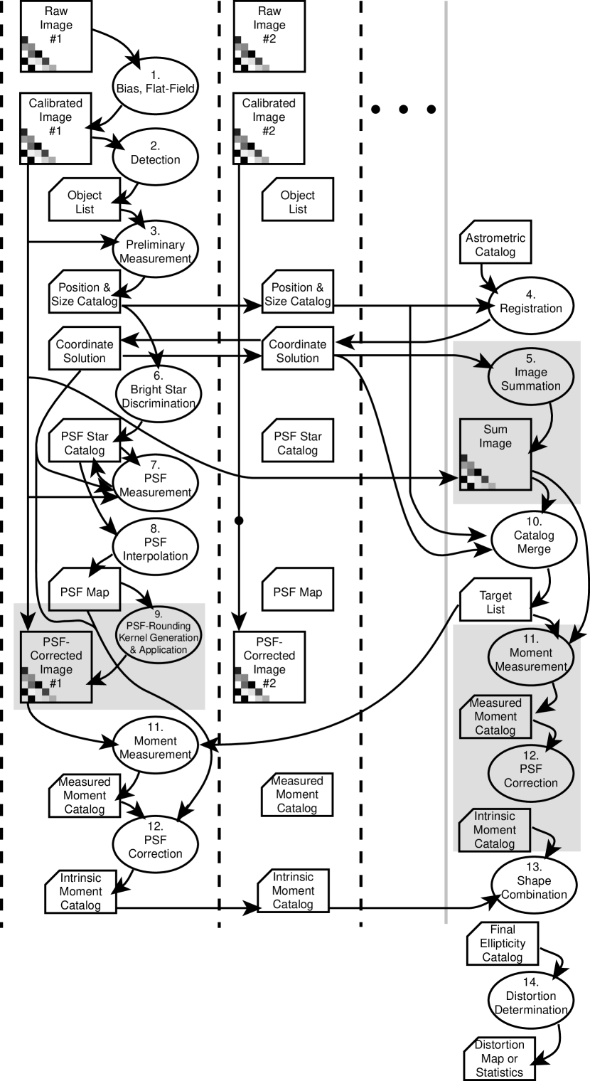
Figure 9: The data flow from raw images through a final lensing distortion map or statistic is illustrated here, with each step described in §9. Shaded regions represent steps that may not be used in all circumstances. Implementation details will be presented in Jarvis et al. (2002)

9.1 Exposure Processing

The steps listed in this section must be performed on each exposure. For mosaic detectors, these steps should be done separately for each channel of the detector if the PSF may change abruptly at the boundaries between detectors.

1. Bias Subtraction and Flat-Fielding: These can be done in the usual fashion. Note that field distortion leads to significant variation in pixel area in many CCD cameras. If the flat-field image is, as usual, obtained by exposing a source of uniform brightness, then the flattened pixel data are a properly calibrated map of the surface brightness of the sky rather than a map of the flux from the sky. This is actually what we want, though it means that simple aperture photometry will lead to incorrect flux estimates.

2. Object Detection: Available detection packages such as FOCAS (Valdes, 1982), SExtractor (Bertin & Arnouts, 1996), or ProFit (P. Fischer, private communication) can be used to identify all objects on the exposure with significance $\nu\gtrsim 3$ and produce a catalog with preliminary position, size, and ellipticity estimation. Each of these packages also produces a useful estimate of total magnitude, which we will preserve. The choice of object detection package is not critical, because the objects that will have useful shape information have sufficiently high significance that any decent detection algorithm will work.

3. Preliminary Measurement: Our shape-measurement algorithm is applied to each detected object in order to obtain an accurate Gaussian-weighted estimate of centroid, size (i.e. the $\sigma$ which maximizes significance), and shape. Objects with saturated or bad pixels are flagged at this point.

4. Registration: The map from pixel coordinates ${\bf x}_{p}$ to the global celestial coordinate grid ${\bf x}$ is established by fitting the measured centroid of the bright objects to a collective catalog (e.g. the average of all individual exposures’ catalogs) and/or an astrometric catalog. This step is critical as even slight misregistrations will produce a systematic coherent ellipticity to the summed images. The photometric offsets between images are determined at this point as well.

5. Image Summation (optional): The exposures can now be remapped to a common grid and photometric scale and summed to give a deeper image. If the flattened images are surface-brightness maps as described in Step 1, then a simple interpolation can be done when remapping the images—no Jacobian flux corrections are needed. Recall the caveats about image combination in §4.1. If shapes are to be measured from the summed image, then we must at this point reconstruct the preliminary catalog by executing Steps 2 and 3 on the summed image.

6. Identification of Stars: As many unsaturated stellar images as possible should be identified on the image for use in PSF determination. Stars are typically identified on the size-magnitude plane. This is a difficult task to execute without excessive human intervention; we want our star-finding algorithm to be flexible enough to identify stars successfully in the presence of a spatially varying PSF, but strict enough to insure that galaxies are not counted as stars. Failure on either count will lead to an erroneous estimate of the PSF size and shape on some part of the exposure, which will lead to a false feature in the shear field. Our algorithms for star identification are described in Jarvis (2002). The algorithms are particularly suited to identifying stars in the presence of a spatially varying PSF size.

7. PSF Measurement: The shape-measurement algorithms are now applied to the identified stars. The integrals in Equation (6-16) give ${\bf b}^{\star}$ at the location of each star. Note that the integral can readily be executed in the global coordinate system ${\bf x}$ because we know the map from pixel coordinates, and because pixel data are already in terms of surface brightness $I$. Thus the effects of image distortion are removed at this step.

8. PSF Interpolation: With the PSF ${\bf b}^{\star}$ measured at the locations of the stars, we need to fit a function ${\bf b}^{\star}({\bf x})$ which describes the PSF at any location on the image. We use a polynomial to describe the variation of each $b^{\star}_{pq}$ across the image. Note that for complex or undersampled PSFs (such as those on HST), interpolation of the $b^{\star}_{pq}$ components is much easier and more accurate than interpolating a pixel-wise representation. In any case this step is again critical: the interpolation scheme must be flexible enough to follow PSF variation, but must remain well-behaved at the image edges and in regions where PSF stars are sparse. There must also be some form of outlier rejection for PSF stars that have cosmic rays or near neighbors contaminating the measurement, but a true excursion of the PSF in some part of the image must not be rejected.

9. PSF-Rounding Kernel (optional): At this point we derive and apply the kernel to remove the anisotropy from the PSF, if desired. Our method for doing so is described in §7. After the convolution it is necessary to repeat Steps 7 and 8 so as to have an updated map of the PSF.

9.2 Object Measurement

We next outline the procedures which yield a shape estimate for every object in the field.

1. Creation of Target Catalog: A list of all targets for shape measurement must be compiled. If there are $\lesssim 5$ exposures of each object, then a master target list can be produced by taking the union of the individual exposure catalogs produced in Step 2. One can use a very low detection threshold on the individual exposures, then guard against noise detections by demanding coincidence on 2 or more exposures. If there are $\gtrsim 5$ exposures per object, then it will be necessary to run a detection algorithm on a summed image in order to find all the potentially useful target galaxies. The target catalog should include an estimate of the centroid (in global coordinates) and some observed size $s_{o}$ of each object. To avoid Kaiser’s selection bias (§8), the criterion for acceptance into the catalog must be some shape-independent statistic.

The following steps are performed for each object in the target catalog:

1. Measurement of Observed Moments: Given the global coordinates of the object, one can determine all of the exposures on which it should appear. Note that for low-significance objects, this may include exposures for which the object was missed in the preliminary detection of Step 2. We then use Equation (6-16) to measure the Laguerre expansion ${\bf b}^{o}$ of the image as observed on each exposure. Once again the integrals are performed in the global coordinate system to remove the effects of optical distortions. The integrals require choice of a centroid and a size parameter $\sigma_{o}$ for the basis functions $\psi_{pq}^{\sigma}$. We may use the approximate centroid from the target catalog, and set the weight size $\sigma_{o}$ equal to the typical observed object size $s_{o}$ from the target catalog. The covariance matrix for the ${\bf b}^{o}$ vector has the diagonal form given in Equation (6-17) for sky-dominated galaxies. Measurements contaminated by saturated pixels or other defects may be rejected at this step.

2. Correction for PSF Effects: There are two methods available here. The first sequence may be used if the rounding kernel has been applied to remove the PSF bias. In this case, if the significance on the individual exposure is $\gtrsim 3$, we may proceed as follows:

   1. Shape Measurement: The image can be shifted, dilated, and sheared until it passes the centroid, significance, and roundness criteria embodied by Equations (6-19)–(6-21). This yields an optimal measure of the observed ellipticity ${\bf e}^{o}$. If the object is of significance $\nu_{0}\gtrsim 3$ on the individual exposure, then we can solve for centroid and size on each exposure independently and still ignore the higher-order terms in the uncertainty of Equation (4-1).

   2. Centroid Bias Correction: Each measured ellipticity must be corrected for the centroid bias (§8) using an empirical value of $K$ in Equation (8-1).

   3. Dilution Correction: The PSF is interpolated to the position of this object to determine the resolution parameter $R$ (Equation [6-1]) or the higher-order version derived in Appendix C. The correction for dilution to give the image-plane (pre-seeing) ellipticity is then simply ${\bf e}^{i}={\bf e}^{o}/R$. The uncertainty ellipse for ${\bf e}$ (Equation [3-30]) is therefore also scaled by $1/R$. Note that it is possible to obtain $e^{i}>1$ if the noise makes the target appear smaller than the PSF.

   4. Averaging of Exposures: The ${\bf e}^{i}$ from the collection of exposures are averaged using the weighting procedures of §4.2. Some form of outlier rejection is necessary to remove objects contaminated by cosmic rays or other defects.

   If we are to perform the PSF bias correction analytically, or if the significance per exposure is low, then it is best to average the deconvolved moments rather than deriving ${\bf e}^{i}$ for each exposure:

   1. Deconvolution of Moments: The PSF decomposition ${\bf b}^{\star}$ is interpolated to the position of the object, and the form of the convolution matrix ${\bf C}({\bf b}^{\star})$ is calculated using the coefficients in Appendix B. This matrix is truncated at some order $p+q\leq N$ and inverted; the deconvolved (pre-seeing) Laguerre decomposition is ${\bf b}^{i}={\bf C}^{-1}\cdot{\bf b}^{o}$. Since this is a linear operation on ${\bf b}$, the covariance matrix for ${\bf b}^{i}$ can be propagated from the simple diagonal covariance matrix for ${\bf b}^{o}$ (Equation [6-17]). There is a subtlety involved in the choice of weight scale $\sigma_{o}$: in §6.2 we determined that the ideal weight scale for the deconvolved image is $\sigma_{i}^{2}=s_{i}^{2}+\sigma_{\star}^{2}=s_{o}^{2}$, where $s_{i}$ and $s_{o}$ are the sizes of the pre- and post-seeing objects, and $\sigma_{\star}$ is the size of the PSF. The typical value of $s_{o}$ was placed in the target catalog in Step 10. According to Equation (6-63), our deconvolution formulae are simplest if we choose the weight scale by

      $$\sigma_{o}^{2}=\sigma_{i}^{2}+\sigma_{\star}^{2}=s_{o}^{2}+\sigma_{\star}^{2}.$$ (9-1)

      Thus in Step 11 we in fact want to use a weight scale somewhat larger than the $s_{o}$ which maximizes the significance of detection.

   2. Combination of Moments: From each exposure we have estimated a ${\bf b}^{i}$ deconvolved moment vector, with known covariance matrix. We average these vectors to obtain a single best estimate of ${\bf b}^{i}$. We have a choice of weights to apply in producing the average; an obvious choice is to weight each exposure inversely with ${\rm Cov}(b_{20}^{i}\bar{b}_{20}^{i})$, since $b_{20}$ carries most of the shape information. Again some form of outlier rejection is necessary at this step.

   3. Symmetrization of Noise: Certain elements of the propagated covariance matrix for the ${\bf b}$ vector must be zero in order to avoid noise anisotropies that produce centroid bias (§8). This can be achieved by selectively adding Gaussian noise to various elements of the combined moment vector.

   4. Determination of Shape: Given the average of ${\bf b}^{i}$ from all exposures, we find the translation and shear that must be applied to satisfy the centroid and roundness conditions $b_{10}=b_{20}=0$. The formulae of Appendix A are used for this. The covariance matrix for ${\bf b}^{i}$ can be propagated through the transformations as well. The uncertainty in the shape $\eta$ is then the square root of ${\rm Var}(b_{20}\bar{b}_{20})/(b_{00}^{2})$. Note that we do not want to maximize the significance by dilating to set $b_{11}=0$. Our optimization criterion is that the shape have minimal error after our transformations. One could dilate the image to satisfy this desire, but our choice of $\sigma_{i}$ should already have us close to the optimum, according to the arguments of §6.2.

   After either of these procedures, we have a measure of the deconvolved shape along with its uncertainty.

3. Combination of Different Wavelengths: If we have imaged the field in a variety of filters, then we will have obtained a shape measurement in each filter. The galaxy’s shape and moments may depend upon wavelength so we don’t want to average together images or moments measured in different filters. We can, however, use the methods of §4.2 to produce a wavelength-averaged ${\bf e}^{i}$ which is maximally sensitive to shear. Weighting each filter by the error in its measured shape insures that we obtain the most sensitivity from each galaxy regardless of its color.

After completion of all these steps, we have a catalog of all objects in the field, specifying their location, magnitude, optimal shape measurement, and shape uncertainty.

9.3 Determination of Shear

With the shape catalog in hand we are close to the scientific goals. The remaining step is

1. Generation of Shear Data: The target galaxies are binned by position, etc., into subsets for which we wish to determine a shear. The shapes (and their uncertainties) may have to be rotated, e.g. into tangential coordinates about some mass center, depending upon the shear statistic under study. The formulae of §5 take the collection of shapes and uncertainties and allow us to create an optimal shear estimate, as well as to propagate the uncertainties in shape to the shear measurement.

10 Conclusions

We have attempted to produce, as rigorously as possible, an end-to-end methodology for measuring gravitational distortion that has optimally low noise, with calibration and noise levels derivable entirely from the observations themselves. We have succeeded in many, but not all, aspects of the problem:

• The measurement of individual galaxy shapes appears to be optimal and has traceable noise characteristics; indeed there even appears to be a straightforward way to handle undersampled data and retain proper covariance information for the intrinsic Laguerre coefficients $b^{i}_{pq}$ (§6.4). The Gaussian weights underlying the Laguerre decomposition are nearly optimal for sky-dominated exponential-profile galaxies. We may wish to reexamine this scheme for the case of when the galaxy is brighter than the sky background.

• The correction of measured moments for the distorting and diluting effects of the PSF can be effected to arbitrary accuracy using the Laguerre-decomposition methods. There will be a tradeoff between elimination of systematic errors—which pushes toward inclusion of higher-order terms in the deconvolution—and the minimization of measurement noise from high-frequency terms. It is not clear if the Laguerre method is optimal with, for example, Airy PSFs with sharp cutoffs in $k$ space; but the method should be better than those yet applied.

• We have identified methods to work around two sources of bias that arise from PSF ellipticities even in the presence of perfect deconvolution.

• Measurements of galaxy shapes from different exposures or filter bands can be optimally combined with standard least-squares techniques, since we know the ${\bf e}$ uncertainty from each individual exposure.

• The determination of lensing distortion from the ensemble of galaxy shapes has a straightforward, optimal, calibratable solution in the case of no measurement noise. In the presence of measurement noise, however, it is necessary to have some knowledge of the noiseless shape distribution to get the calibration factor exactly correct. Our approximations, however, seem to suffice to get accuracies of 5–10%.

A detailed performance comparison of our methods with other authors’ is beyond the scope of the paper. We can guess, however, that the reduction of measurement noise relative to a carefully weighted implementation of KSB will be slight, perhaps a factor of 1.5. But our methods, like those of K00 and Refregier (2001), are formally valid for any reasonable PSF, and hence we expect to have much-reduced systematic errors. Indeed it is likely that the biases of §8 have not been extensively tested because they were lost under the larger errors in PSF correction (as also noted by K00).

Our methods share elements with many previous proposals. An aesthetic difference is that we retain the geometric meaning of ellipticity by, in effect, using adaptively shaped weights instead of fixed circular weights. This makes the “shear polarizability” a purely geometric effect. As a consequence we can examine the $P(e)$ distributions and find ways to exploit surface brightness, $b_{22}$, or color information to separate the spheroid galaxies and weight them more heavily to reduce the shape noise.

It will be of interest to see how our method compares to the commutator method of K00. One would hope that the two independent methods could be applied to the same dataset and yield the same results, bolstering our confidence in these very difficult measurements.

In a succeeding paper (Jarvis et al., 2002) we will present some of the implementation details for the analytical methods here, and test the methods on real and simulated data. Fischer et al. (2000); Smith et al. (2000); Wittman et al. (2000) make use of portions of this methodology, so the systematic-error tests and calibration tests in those papers already serve as demonstrations. Upcoming precision measurements of cosmic shear will make even greater demands upon the systematic-error reduction and accurate calibration that our methods offer.

Appendix A Point Transformation for Laguerre Expansions

In §6.3.2 we derived the mapping matrices for the vector ${\bf b}$ of Laguerre-expansion coefficients when the underlying image $I$ is transformed by an infinitesimal translation, dilation, or shear. In this Appendix we derive the coefficients of the mapping matrices for finite transformations. We have implemented these transformations as methods for C++ classes that represent the Laguerre expansions.

A.1 Translation

We defined the transformation ${\bf T}_{z}$ on the image by

$${\bf T}_{z}I(x,y) = I(x-x_{0},y-y_{0})$$ (A1)

$$z \equiv {{x_{0}+iy_{0}}\over\sigma}.$$ (A2)

We first define a translated raising operator $\hat{a}_{p}^{\sigma\dagger}$ by

$$\hat{a}_{p}^{\sigma\dagger}({\bf T}_{z}I) \equiv {\bf T}_{z}(a_{p}^{\sigma\dagger}I)$$ (A3)

$$\Rightarrow\quad\hat{a}_{p}^{\sigma\dagger} = a_{p}^{\sigma\dagger}-{z\over 2}.$$ (A4)

The second line is apparent from examining the form of the raising operators in Equation (6-22). We decompose the images into our eigenfunctions as $I=\sum b_{pq}\psi_{pq}^{\sigma}$ and ${\bf T}_{z}I=\sum b^{\prime}_{pq}\psi_{pq}^{\sigma}$; then we can express ${\bf T}_{z}$ as a matrix operation on ${\bf b}$:

$${\bf b^{\prime}} = {\bf T}_{z}\cdot{\bf b}$$ (A5)

$$b^{\prime}_{p^{\prime}q^{\prime}} = \sum T_{p^{\prime}q^{\prime}}^{pq}b_{pq}$$ (A6)

$${\bf T}_{z}\psi_{pq}^{\sigma} = \sum T_{p^{\prime}q^{\prime}}^{pq}\psi^{\sigma}_{p^{\prime}q^{\prime}}.$$ (A7)

$$\Rightarrow\quad T_{p^{\prime}q^{\prime}}^{pq} = \sigma^{2}\int\!d^{2}\!x\,({\bf T}_{z}\psi_{pq}^{\sigma})\bar{\psi}^{\sigma}_{p^{\prime}q^{\prime}}.$$ (A8)

A direct integration of (A8) yields the first coefficient

$$T_{00}^{00}=e^{-|z|^{2}/4}.$$ (A9)

Applying the translated raising operator (A4) to the definition (A7) of $T_{p^{\prime}q^{\prime}}^{pq}$ yields the recursion relation

$$\sqrt{p^{\prime}}\,T_{(p^{\prime}-1)q^{\prime}}^{pq}-{z\over 2}\,T_{p^{\prime}q^{\prime}}^{pq}=\sqrt{p+1}\,T_{p^{\prime}q^{\prime}}^{(p+1)q}.$$ (A10)

The same procedure using the $q$ raising operator and the lowering operators gives the recursions

$$\sqrt{q^{\prime}}\,T_{p^{\prime}(q^{\prime}-1)}^{pq}-{\bar{z}\over 2}\,T_{p^{\prime}q^{\prime}}^{pq} = \sqrt{q+1}\,T_{p^{\prime}q^{\prime}}^{p(q+1)}$$ (A11)

$$\sqrt{p^{\prime}+1}\,T_{(p^{\prime}+1)q^{\prime}}^{pq}-{\bar{z}\over 2}\,T_{p^{\prime}q^{\prime}}^{pq} = \sqrt{p}\,T_{p^{\prime}q^{\prime}}^{(p-1)q}$$ (A12)

$$\sqrt{q^{\prime}+1}\,T_{p^{\prime}(q^{\prime}+1)}^{pq}-{z\over 2}\,T_{p^{\prime}q^{\prime}}^{pq} = \sqrt{q}\,T_{p^{\prime}q^{\prime}}^{p(q-1)}$$ (A13)

These two relations allow us to generate any $T_{p^{\prime}q^{\prime}}^{pq}$ recursively from $T_{00}^{00}$. In particular, using the first 2 we have

$$T_{00}^{pq}={{(-1/2)^{p+q}}\over\sqrt{p!q!}}z^{p}\bar{z}^{q}e^{-|z|^{2}/4}.$$ (A14)

One can derive a closed-form expression for the general $T_{p^{\prime}q^{\prime}}^{pq}$ using further recursion, but the expression involves a double sum and is not particularly illuminating. The most efficient algorithm for computing all the coefficients is to note that the generator for translation (Equation [6-38]) separates into $p$- and $q$-dependent components. The general matrix element can therefore be expressed as

$$T_{p^{\prime}q^{\prime}}^{pq}=f(p,p^{\prime})\bar{f}(q,q^{\prime}),$$ (A15)

with the above recursion relations for $T_{p^{\prime}q^{\prime}}^{pq}$ leading to

$$f(p,0) = {{(-z/2)^{p}}\over\sqrt{p!}}e^{-|z|^{2}/8},$$ (A16)

$$f(p,p^{\prime}+1) = \left[\sqrt{p}\,f(p-1,p^{\prime})+{\bar{z}\over 2}f(p,p^{\prime})\right]/\sqrt{p^{\prime}+1}$$ (A17)

A.2 Dilation

The dilation operation is defined by

$${\bf D}_{\mu}I(x,y)=I(e^{-\mu}x,e^{-\mu}y)$$ (A18)

As for the translation, we can define a dilated raising operator and use it to derive a recursion relation for the coefficients of ${\bf D}$:

$$\hat{a}_{p}^{\sigma\dagger}({\bf D}_{\mu}I) = {\bf D}_{\mu}(a_{p}^{\sigma\dagger}I)$$ (A19)

$$\Rightarrow\quad\hat{a}_{p}^{\sigma\dagger} = \cosh\mu\,a_{p}^{\sigma\dagger}-\sinh\mu\,a_{q}^{\sigma}$$ (A20)

$$\Rightarrow\quad\sqrt{p+1}\,D_{p^{\prime}q^{\prime}}^{(p+1)q} = \cosh\mu\,\sqrt{p^{\prime}}\,D_{(p^{\prime}-1)q^{\prime}}^{pq}-\sinh\mu\,\sqrt{q^{\prime}+1}\,D_{p^{\prime}(q^{\prime}+1)}^{pq}$$ (A21)

Using the recursion operator and its $q$ equivalent, we can generate any desired coefficient from $D_{pq}^{00}$. With the direct integration analogous to Equation (A8), we derive

$$D_{pq}^{00}=e^{\mu}{\rm sech}\mu(\tanh\mu)^{p}\,\delta_{pq}.$$ (A22)

In deriving this we make use of the identity (Abramowitz & Stegun, 1965)

$$L_{q}^{(m)}(\alpha x)=\sum_{k=0}^{q}{q+m\choose q-k}\alpha^{k}(1-\alpha)^{q-k}L_{k}^{(m)}(x).$$ (A23)

In fact with this identity one can derive any $D_{p^{\prime}q^{\prime}}^{pq}$ by direct integration, but the closed form is a sum over $k$ that is again not particularly useful, as the recursion relation (A21) is a faster way to generate the coefficients.

A.3 Shear

A shear $\eta$ oriented on the $x$ axis gives the transformation

$${\bf S}_{\eta}I(x,y)=I(e^{-\eta/2}x,e^{\eta/2}y).$$ (A24)

When we define the transformed raising operator $\hat{a}_{p}^{\sigma\dagger}$ as for the translation and dilation, we find the operator and consequent recursion relation to be

$$\Rightarrow\quad\hat{a}_{p}^{\sigma\dagger} = \cosh(\eta/2)\,a_{p}^{\sigma\dagger}-\sinh(\eta/2)\,a_{p}^{\sigma}$$ (A25)

$$\Rightarrow\quad\sqrt{p+1}\,S_{p^{\prime}q^{\prime}}^{(p+1)q} = \cosh(\eta/2)\,\sqrt{p^{\prime}}\,S_{(p^{\prime}-1)q^{\prime}}^{pq}-\sinh(\eta/2)\,\sqrt{p^{\prime}+1}\,S_{(p^{\prime}+1)q^{\prime}}^{pq}.$$ (A26)

The recursion again simplifies by noting that the shear generator in Equation (6-33) separates into $p$ operands and $q$ operands. Hence the matrix elements must be expressible as $S^{pq}_{p^{\prime}q^{\prime}}=f(p,p^{\prime})f(q,q^{\prime})$. We can determine the function $f(p,0)$ by direct integration of the $S_{00}^{p0}$ matrix element, which yields (for $p$ even)

$$S_{00}^{p0} = {\sqrt{p!}\over{(p/2)!}}{\rm sech}(\eta/2)\left({{-\tanh(\eta/2)}\over 2}\right)^{p/2}$$ (A27)

$$\Rightarrow\quad S_{00}^{pq} = {\sqrt{p!q!}\over{(p/2)!(q/2)!}}{\rm sech}(\eta/2)\left({{-\tanh(\eta/2)}\over 2}\right)^{(p+q)/2}.$$ (A28)

The coefficients vanish if $p$ or $q$ are odd. The recursion relation then generates any desired coefficient. For a shear oriented at position angle $\beta$, the coefficients acquire an additional phase factor $\exp[i(p^{\prime}-q^{\prime}-p+q)\beta]$.

Appendix B Convolution of Laguerre Expansions

We wish to derive the coefficients which express the convolution of two eigenfunctions as a new sum over eigenfunctions, as defined in Equation (6-57). This will be easier if we work in $k$ space, with the convolution turned into a multiplication as in Equation (6-59), with the $k$-space eigenfunctions given in Equation (6-62).

A rapidly computable recursive formulation of the coefficients is again derivable from the raising operator. From the form of the $k$-space raising operator (6-61) we see that if $\sigma_{o}^{2}=\sigma_{i}^{2}+\sigma_{\star}^{2}$, then

$$\sigma_{o}\tilde{a}_{p}^{\sigma_{o}\dagger}\tilde{I}_{o} = (\sigma_{i}\tilde{a}_{p}^{\sigma_{i}\dagger}\tilde{I}_{i})\tilde{I}_{\star}+\tilde{I}_{i}(\sigma_{\star}\tilde{a}_{p}^{\sigma_{\star}\dagger}\tilde{I}_{\star})$$ (B1)

$$\Rightarrow\quad\sigma_{\star}\sqrt{p_{\star}+1}\,C_{p_{o}q_{o}}^{p_{i}q_{i}(p_{\star}+1)q_{\star}} = \sigma_{o}\sqrt{p_{o}}\,C_{(p_{o}-1)q_{o}}^{p_{i}q_{i}p_{\star}q_{\star}}-\sigma_{i}\sqrt{p_{i}+1}\,C_{p_{o}q_{o}}^{(p_{i}+1)q_{i}p_{\star}q_{\star}}.$$ (B2)

An equivalent manipulation with the lowering operator yields the recursion relation

$$\sigma_{o}\sqrt{p_{o}}\,C_{(p_{o}+1)q_{o}}^{p_{i}q_{i}p_{\star}q_{\star}}=\sigma_{i}\sqrt{p_{i}}\,C_{p_{o}q_{o}}^{(p_{i}-1)q_{i}p_{\star}q_{\star}}+\sigma_{\star}\sqrt{p_{\star}}\,C_{p_{o}q_{o}}^{p_{i}q_{i}(p_{\star}-1)q_{\star}}.$$ (B3)

These recursion relations, and their $q$ equivalent, will allow us to derive any coefficient if we know $C_{p_{o}q_{o}}^{p_{i}q_{i}00}$, i.e. if we can calculate the effect of multiplication by the Gaussian $\tilde{\psi}_{00}^{\sigma_{\star}}$. This is straightforward if we recall that $m_{o}=m_{i}$ for $m_{\star}=0$, and use Equation (A23):

$$2\pi\tilde{\psi}_{p_{i}q_{i}}^{\sigma_{i}}\tilde{\psi}_{00}^{\sigma_{\star}} = 2\sqrt{\pi}\sum_{p_{o}=0}^{p_{i}}\sum_{q_{o}=0}^{q_{i}}\sqrt{{p_{i}!q_{i}!}\over{p_{o}!q_{o}!}}{{D^{(p_{o}+q_{o})/2}(1-D)^{q_{i}-q_{o}}}\over(q_{i}-q_{o})!}\tilde{\psi}_{p_{o}q_{o}}^{\sigma_{o}}$$ (B4)

$$\Rightarrow\quad C_{p_{o}q_{o}}^{p_{i}q_{i}00} = 2\sqrt{\pi}\sqrt{{p_{i}\choose p_{o}}{q_{i}\choose q_{o}}}D^{(p_{o}+q_{o})/2}(1-D)^{(p_{i}-p_{o}+q_{i}-q_{o})/2},$$ (B5)

$$D \equiv {\sigma_{i}^{2}\over\sigma_{o}^{2}}={\sigma_{i}^{2}\over{\sigma_{i}^{2}+\sigma_{\star}^{2}}}=1-{\sigma_{\star}^{2}\over\sigma_{o}^{2}}.$$ (B6)

The parameter $D$ is the “deconvolution ratio,” with $D=1$ being the limit of perfect resolution and $D=0$ meaning a PSF much broader than the image. This expression and the recursion relations are both separable into $p$- and $q$-dependent terms, so we can simplify the computation of the matrix elements by using the expression

$$C_{p_{o}q_{o}}^{p_{i}q_{i}p_{\star}q_{\star}} = 2\sqrt{\pi}\left[\sqrt{p_{i}!p_{\star}!\over p_{o}!\Delta!}G(p_{o},p_{i},p_{\star})\right]\left[\sqrt{q_{i}!q_{\star}!\over q_{o}!\Delta!}G(q_{o},q_{i},q_{\star})\right]$$ (B7)

$$\Delta \equiv p_{i}+p_{\star}-p_{o}=q_{i}+q_{\star}-q_{o}\geq 0.$$ (B8)

Terms for which the conditions in the second line are not met are zero. The recursion relations and specific values given above for $C$ can be recast for the function $G$ as follows:

$$G(p_{o}+1,p_{i},p_{\star}) = {\sigma_{i}\over\sigma_{o}}G(p_{o},p_{i}-1,p_{\star})+{\sigma_{\star}\over\sigma_{o}}G(p_{o},p_{i},p_{\star}-1)$$ (B9)

$$G(0,p_{i},p_{\star}) = (-1)^{p_{\star}}{p_{i}+p_{\star}\choose p_{i}}\left({\sigma_{i}\over\sigma_{o}}\right)^{p_{\star}}\left({\sigma_{\star}\over\sigma_{o}}\right)^{p_{i}}$$ (B10)

The symmetry between initial and PSF images is clear in these equations. There is a consequent closed form for $G(p_{o},p_{i},p_{\star})$, but it is again not particularly illuminating, and the recursive form is stable and faster for computation.

In the case where the PSF is a unit-flux Gaussian, Equation (B5) can be used to give the observed ${\bf b}^{o}$ in terms of the intrinsic decomposition:

$$b^{o}_{p_{o}q_{o}}=\sum_{j=0}^{\infty}D^{(p_{o}+q_{o})/2}\sqrt{{p_{o}+j\choose p_{o}}{q_{o}+j\choose q_{o}}}(1-D)^{j}b^{i}_{(p_{o}+j)(q_{o}+j)}\qquad(p_{o}\geq q_{o}).$$ (B11)

Note that the convolution matrix ${\bf C}$ is in this case block-diagonal, as the $m$ states do not mix, and also upper triangular, as $p_{o},q_{o}\leq p_{i},q_{i}$ for non-zero elements. The inverse (deconvolution) matrix can in this case be expressed in closed form:

$$b^{i}_{p_{i}q_{i}}=\sum_{j=0}^{\infty}D^{-(p_{i}+q_{i})/2}\sqrt{{p_{i}+j\choose p_{i}}{q_{i}+j\choose q_{i}}}\left({{1-D}\over D}\right)^{j}(-1)^{j}b^{o}_{(p_{i}+j)(q_{i}+j)}.$$ (B12)

Appendix C Second-order Formulae for PSF Dilution

Here we describe a refinement to the resolution parameter $R$ defined in Equation (6-1). The observed ellipticity is $R$ times the true ellipticity in the special cases of unweighted moments or when the PSF is a circular Gaussian and the galaxy an elliptical Gaussian. In these cases the factor $R$ can be expressed as

$$R = 1-{s^{2}_{\star}\over s^{2}_{o}},$$ (C1)

$$s^{2} \equiv \langle(x^{2}+y^{2})/2\rangle=\sigma^{2}\cosh\eta.$$ (C2)

In the second line we have assumed that the methods of §3 have been used to shear the object by $\eta$ to produce something that is “round” under a Gaussian weight of optimal size $\sigma$.

Here we derive a form for $R$ which is applicable to the case in which the galaxy has homologous elliptical isophotes with $\eta\ll 1$, but with an arbitrary radial profile. In the language of our Laguerre coefficients, we have $b_{11}=0$ by proper choice of $\sigma$, and $b_{pp}$ are arbitrary for $p\geq 2$. By Equation (6-34) this slightly out-of-round object has $b_{20}=\sqrt{2}\eta(b_{00}-b_{22})/4$. All odd-indexed coefficients are zero.

We also take the PSF size $\sigma_{\star}$ to be small compared to the intrinsic object size $\sigma_{i}$. The action of this small isotropic convolution ${\bf C}_{\sigma_{\star}}$ on the moments is the same as a transformation in which the image $I$ is replaced by the average of two versions displaced by $\pm\sigma_{\star}$ in the $x$ direction, followed by a similar infinitesimal spread in the $y$ direction. Defining $z=\sigma_{\star}/\sigma$ and using a second-order version of the generator Equation (6-38), we can show that

$${\bf C}_{\sigma_{\star}} = {1\over 4}\left({\bf T}_{z}+{\bf T}_{-z}\right)\left({\bf T}_{iz}+{\bf T}_{-iz}\right)$$ (C3)

$$\approx 1+{z^{2}\over 2}\left[a_{p}^{\dagger}a_{q}^{\dagger}+a_{p}a_{q}-p-q-1\right]$$ (C4)

When this convolution acts upon our original slightly-elliptical object, the resulting object has Laguerre coefficients ${\bf b}^{\prime}$ with

$$b^{\prime}_{00} = b_{00}(1-z^{2}/2)$$ (C5)

$$b^{\prime}_{20} = b_{20}(1-3z^{2}/2)$$ (C6)

$$b^{\prime}_{22} = b_{22}(1-5z^{2}/2)$$ (C7)

We then need the value $\eta^{\prime}$ of the shear that will make this new object appear round. According to Equation (6-47), this will give

$$\eta^{\prime} = {\eta(b_{00}-b_{22})(1-3z^{2}/2)\over 1-z^{2}/2-b_{22}(1-5z^{2}/2)}$$ (C8)

$$\Rightarrow\qquad R\equiv{\eta^{\prime}\over\eta} = 1-z^{2}\left(1+{2b_{22}\over b_{00}-b_{22}}\right)+O(z^{4})$$ (C9)

$$\approx 1-{\sigma_{\star}^{2}\over s^{2}},$$ (C10)

$$s^{2} \equiv \sigma^{2}{b_{00}-b_{22}\over b_{00}+b_{22}}.$$ (C11)

Note that the kurtosis measure $a_{4}$ defined in Equation (3-26) is the same as $b_{22}/b_{00}$ which appears here. We make the ansatz that the correct form for $R$ in the case of finite dilution or finite $e$ is the Gaussian form Equation (C1) with the kurtosis term added:

$${\bf e}_{i} = {\bf e}_{o}/R,$$ (C12)

$$R = 1-{s^{2}_{\star}\over s^{2}_{o}},$$ (C13)

$$s^{2} \equiv {1-a_{4}\over 1+a_{4}}\sigma^{2}\cosh\eta.$$ (C14)

Note that we apply the kurtosis correction to the PSF size measure $s^{2}_{\star}$ in the same way as for the object, to give a well-behaved correction for poorly-resolved objects.

References

- Abramowitz & Stegun (1965) Abramowitz, M., & Stegun, I. 1965, Handbook of Mathematical Functions, (New York: Dover)
- Bacon et al. (2000) Bacon, D., Refregier, A., Clowe, D., & Ellis, R. 2000, MNRAS (submitted)
- Bernstein (2001) Bernstein, G. 2001, PASP, (in press)
- Bertin & Arnouts (1996) Bertin, E., & Arnouts, S. 1996, A&AS, 117, 393
- Bonnet, Mellier, & Fort (1994) Bonnet, H., Mellier, Y., & Fort, B. 1994, ApJ, 427, L83
- Bonnet & Mellier (1995) Bonnet, H., & Mellier, Y. 1995, A&A, 303, 331
- Bracewell (1978) Bracewell, R. N. 1978, The Fourier Transfrom and Its Applications (New York: McGraw-Hill)
- Dye et al. (2001) Dye, S., Taylor, A. N., Thommes, E. M., Meisenheimer, K., Wolf, C., & Peacock, J. A. 2001, MNRAS, 321, 685
- Erben et al. (2001) Erbern, T., Van Waerbeke, L., Bertin, E., Mellier, Y., & Schneider, P. 2001, A&A, 366, 717
- Fahlman et al. (1994) Fahlman, G., Kaiser, N., Squires, G., & Woods, D. 1994, ApJ, 437, 56
- Fischer et al. (1997) Fischer, P., Bernstein, G. M.,, Tyson, J. A., & Rhee, G. 1997, AJ, 113, 521
- Fischer & Tyson (1997) Fischer, P., & Tyson, J. A. 1997, AJ, 114, 14
- Fischer et al. (2000) Fischer, P. et al.2000 , AJ, 120, 1193
- Hoekstra et al. (1998) Hoekstra, H., Franx, M., Kuijken, K, & Squires, G. 1998, ApJ, 504, 636
- Hoekstra et al. (2000) Hoekstra, H., Franx, M., & Kuijken, K 2000, ApJ, 532, 88
- Hoekstra et al. (2001) Hoekstra, H. et al. 2001, ApJ, 548, L5
- Jarvis (2002) Jarvis, M. 2002, (in prep.)
- Jarvis et al. (2002) Jarvis, M., Bernstein, G., Fischer, P., & Smith, D. 2002, (in prep.)
- Kaiser (2000) Kaiser, N. 2000, ApJ, 537, 555
- Kaiser, Squires, & Broadhurst (1995) Kaiser, N., Squires, G., & Broadhurst, T. 1995, ApJ, 449, 460.
- Kochanski & Fisher (1994) Kochanski, G. P,, & Fisher, P. 1994, AJ, 107, 802
- Kuijken (1999) Kuijken, K. 1999, A&A, 352, 355.
- Lauer (1999) Lauer, T. R. 1999, PASP, 111, 227
- Lombardi & Bertin (1998) Lombardi, M. & Bertin, G. 1998, A&A, 330, 791.
- Luppino & Kaiser (1997) Luppino, G., & Kaiser, N. 1997, ApJ, 475, 20.
- Mellier (1999) Mellier, Y. 1999, ARA&A, 37, 127
- Miralda-Escudé (1991) Miralda-Escudé, J. 1991, ApJ, 380, 1
- Mould et al. (1994) Mould, J. et al. 1994, MNRAS, 271, 31.
- Refregier (2001) Refregier, A. 2001, astro-ph/0105178
- Refregier & Bacon (2001) Refregier, A. & Bacon, D. 2001, astro-ph/0105179