Wide field weak lensing observations of A1689

We present a mass profile for A1689 from $0.13h^{-1}\mathrm{Mpc}<r<2h^{-1}\mathrm{Mpc}$ from a weak lensing analysis of a $34\arcmin\times 34\arcmin$ $R$-band image from the ESO/MPG Wide Field Imager. We detect the gravitational shearing of a $23<R<25.5$ background galaxy population even at the edge of the image with a $4\sigma$ significance, and find a two-dimensional mass reconstruction has a $13.4\sigma$ significance mass peak centered on the brightest cluster galaxy. This peak is well fit by both a $1028\pm 35$ km/s singular isothermal sphere and a $r_{200}=1.28\>\mathrm{Mpc},c=6$ “universal” CDM profile, although the “universal” CDM profile provides a better fit with 95.5% confidence. These mass measurements are lower than most of those derived by other means and we discuss possible reasons for weak lensing providing an underestimate of the true mass of the cluster. We find that the correction factors needed to reconcile the weak lensing mass models with the strong lensing Einstein radius would result is a much larger fraction of faint stars and foreground and cluster dwarf galaxies in the $23<R<25.5$ object catalog than is seen in other fields.

1 Introduction

Clusters of galaxies provide several methods of constraining cosmological and dark matter models. Two of the most important properties of the clusters in constraining these models are the total mass and the mass profile. The three most common techniques in measuring the masses of clusters are dynamical measurements from the line-of-sight velocity dispersion of cluster galaxies, the X-ray luminosity and temperature of intra-cluster gas, and measurement of the distortion of background galaxy images by the cluster potential. In recent years, the dispersion of the masses measured by the various techniques has been reduced by improved data and the reduction of systematic errors, so that in many clusters the mass measurements are in good agreement. There are a few clusters, however, in which the three mass measurement techniques are not in agreement, one of the most striking of which is Abell 1689.

Abell 1689 is one of the richest clusters ($R=4$) in the Abell catalog, but the number counts may be enhanced by a number of lower redshift groups in the field (Teague et al. 1990). A velocity dispersion of 2355 ${}^{+238}_{-183}$ km/s has been measured from 66 cluster members (Teague et al. 1990), although a more conservative criteria for cluster membership reduced the velocity dispersion to 1848$\pm 166$ km/s (Gudehus 1989). By using a technique which identifies substructure from both redshift and positional information, Girardi et al. (1997) divide the cluster galaxies into three distinct groups each with velocity dispersions of 250-400 km/s, which would coadd to a mass equivalent to an $\approx 560$ km/s isothermal sphere.

A set of giant arcs $\sim 45\arcsec$ from the brightest cluster galaxy (hereafter BCG) provide a best-fit model of a 1400 km/s isothermal sphere centered on the BCG and a 700 km/s isothermal sphere located 1$\arcmin$ northeast of the BCG (Miralda-Escudé & Babul 1995). Analysis of the depletion of background galaxies around the cluster core, due to the deflection and magnification of the galaxies by the gravitational potential, results in a best-fit velocity dispersion of 2200$\pm$500 km/s, but is also well fit by the double isothermal sphere model from strong gravitational lensing (Taylor et al. 1998). An analysis of the change in the background galaxy luminosity function has measured a mass of $(0.48\pm 0.16)\times 10^{15}h^{-1}\mathrm{M}_{\odot}$ at a $0.25h^{-1}\mathrm{Mpc}$ radius from the cluster core, which is consistent with the depletion mass model (Dye et al. 2001). Weak lensing shear analysis of the cluster core gives a mass estimate similar to that of the strong lensing (Kaiser 1996), but suggests that the mass profile is best fit by a power law with index $n=1.4\pm 0.2$ (Tyson & Fischer 1995). X-ray observations give a gas temperature of 9-10 keV and best-fit velocity dispersions of 1000-1400 km/s (Allen 1998).

A standard model used to explain these observations involves one or more structures (second cluster, filament extending along the line of sight, etc) located at a redshift only slightly larger than the cluster (Taylor et al. 1998). This would result in line of sight dynamical velocity dispersion measurement larger than the actual velocity dispersion of the cluster due to the misinterpretation of cosmological redshift to be velocity. It would also result in the lensing mass measurement being higher than the mass of the cluster core as the lensing measures the total mass surface density of all the structures along the line of sight. The X-ray measurements would thus provide the best estimate of the true mass of the cluster core, as the small mass structures would provide only a small perturbation to the cluster X-ray luminosity and gas temperature. If, however, the additional structure is undergoing a merger event with the cluster then the gravitational interaction could create shock heating of the gas and render invalid the assumptions about isothermality and hydrostatic equilibria on which the X-ray models are based. Also, if the Tyson & Fischer (1995) result of the mass profile of the cluster being steeper than that of an isothermal sphere is correct, then the models which convert the dynamical line-of-sight velocity dispersion and X-ray measurements to mass estimates are incorrect. This result, however, is based on a relatively small field and is therefore uncertain due to the mass sheet degeneracy and the breakdown of the weak lensing approximation near the cluster core.

Due to the new wide-field mosaic CCDs (Luppino et al. 1998) it is now possible to obtain a weak lensing signal from low-to-medium redshift clusters out to large radii ($\sim 2h^{-1}$ Mpc) in only a few hours of telescope time. Here we report on observations of A1689 made with the Wide Field Imager on the ESO/MPG 2.2m telescope on La Silla. In Section 2 we discuss the image reduction and object catalog generation. We analyze the weak lensing signal in Section 3. Finally, in Section 4 we compare our mass estimates to others and present our conclusions. Unless otherwise stated we assume a $\Omega_{\mathrm{m}}=0.3,\Lambda=0.7$ cosmology and $H_{0}=100$ km/s/Mpc.

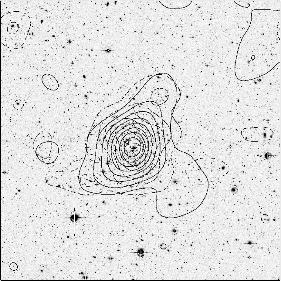
Figure 1: Above is a $33\arcmin\times 33\arcmin$ R-band image of the cluster A1689 from the Wide Field Imager on the ESO/MPG 2.2m telescope plotted using a $\sqrt{\log}$ stretch. The two-dimensional mass reconstruction from the weak lensing shear signal is drawn in solid-line contours. The input shear field was smoothed using a $\sigma=1\aas@@fstack{\prime}2$ Gaussian, which is roughly the smoothing level of the output mass reconstruction. Each contour represents an increase in $\kappa$ of 0.015 above the mean $\kappa$ at the edge of the field. The dashed-line contours show the flux-weighted distribution of galaxies with $16.7<R<22$ also smoothed by a $\sigma=1\aas@@fstack{\prime}2$ Gaussian.

2 Observations and Data Reduction

Twelve 900 second exposures in $R$-band were obtained with the Wide Field Imager (WFI) on the ESO/MPG 2.2m telescope on the night of May 29, 2000. The images were taken with a dithering pattern between exposures which filled in the gaps between the chips in the CCD mosaic. The resulting image covers a $34\aas@@fstack{\prime}7\times 33\aas@@fstack{\prime}4$ area centered on the cluster with $82.5\%$ of the area having the full exposure time and the remaining $17.5\%$ of the area receiving less than the full exposure time due to the area being out of the field of view or in the gap between the chips during some of the exposures. The final image has a FWHM on unsaturated stars of $0\aas@@fstack{\prime\prime}72$ and a $1\sigma$ sky noise of 28.1 mag/sq arcsec on the areas having the full exposure time. Object counts at a $3\sigma$ detection limit in the regions containing the full exposure time are complete to $R=24.9$ for $2\arcsec$ radius aperture magnitudes, as measured by the point where the number counts depart from a power law.

During the image reduction process, each chip in the CCD mosaic was treated separately for the steps detailed below. We first de-biased the images using a master bias taken at the beginning of the night and corrected for bias drift in each exposure using the overscan strip. The images were then flattened by a polynomial fit to a twilight flat taken during the evening twilight. The polynomial fitting was done using a 9th by 17th order two-dimensional polynomial $f(x,y)=\sum_{l=0}^{9}\sum_{m=0}^{17}a_{lm}x^{l}y^{m}$ with $a_{lm}=0$ if $(l/9)^{2}+(m/17)^{2}>1$ to accurately mimic the large-scale variations in quantum efficiency while removing the small scale variations in the twilight flat caused by fringing. The ratio of powers in the $x$ and $y$ directions were chosen so as to have the same density of inflection points in the polynomial across the rectangular CCD. A medianed nightsky flat was then made from all of the long-exposure, twilight-flattened $R$-band images taken that night. The nightsky flat showed a peak-to-peak fringing amplitude of $\sim 10\%$ ($[\mathrm{max}-\mathrm{min}]/[0.5\times(\mathrm{max}+\mathrm{min})]\sim 0.1$ in adjacent minima and maxima).

We tried two different techniques to remove the fringing and flatfield the images with the nightsky flat. The first technique was to fit the nightsky flat with a 9th by 17th order two-dimensional polynomial and flatten the images with the polynomial. The flattened images were then medianed to produce another nightsky flat, which was assumed to contain only the fringing pattern. This fringing pattern was then scaled to the sky level in each image and subtracted. The second technique was to simply flatten the images with the original nightsky flat, fringes included. Neither technique is strictly correct as in the former case we are subtracting small-scale changes in the quantum efficiency (dust, chip defects, etc) instead of dividing by them, while in the latter case we are treating the interference-based fringe pattern as a variation in the quantum efficiency. We used both sets of flattened images to create two different final images and performed all further analysis on both images. In each case, the results for both images were statistically identical (differences between the images were at least one order of magnitude smaller than the $1\sigma$ error bars of the measurement). For the rest of the paper we discuss only the results from the first technique image, but none of the conclusions change when using the second technique image.

One problem with the WFI is that bright stars can have several reflection rings, many of which are not centered on the star which causes them. In this field there are 16 stars of sufficient brightness to cause noticeable reflection rings on the final image. Each star has two small rings, outer radii $\approx 48\arcsec$, offset from each other by a few pixels. These rings are typically a few arcseconds from the star radially away from the center of the field, with the separation getting larger with the star’s distance from the field center. The brightest five stars also have a much fainter third ring, outer radius $\approx 92\arcsec$, which is centered about twice as far from the star as the smaller rings in the same radial direction. These reflection rings have structure not only in both radial and tangential directions from the center of the ring, but also random structures similar to, and probably caused in part by the removal of, the fringing in the sky. As a result, we were unable to remove these rings while preserving the haloes of any objects inside them. The regions containing the reflections rings were therefore removed from all further analysis below.

The sky level of each image was determined by detecting minima in a smoothed image, and fitting the minima with a 7th by 15th order two-dimensional polynomial. The resulting sky fit was subtracted from each image, which allowed the removal of extended haloes from saturated stars without affecting the profiles of individual galaxies.

The next step in the image reduction was to move each image into a common reference frame while simultaneously removing any distortion in the image introduced by the telescope optics. To do this we assumed that each CCD of the mosaic could be mapped onto a common detector plane using only a linear shift in the $x$ and $y$ directions and a rotation angle in the $x$-$y$ plane, and that these mappings are the same for each image. In doing so we assume that the detectors are aligned well vertically and thus no change in the platescale, distortion, etc. occurs across chip boundaries and that the chips do not move relative to each other while the instrument is subjected to thermal variations and/or varying flexure from pointing to different parts of the sky. We justify these assumption later using analysis of the resulting PSF ellipticities. We then used a bi-cubic polynomial to map the detector plane for each exposure to a common reference frame. The parameters for the two sets of mapping were determined simultaneously by minimizing the positional offsets of bright, but unsaturated, stars among the various images and with the USNO star catalog. A downhill simplex minimization method was employed to minimize the 21 free parameters in the individual CCDs to detector plane mapping, and at each step the detector plane to common reference plane mapping parameters were determined for each image using LU decomposition of a $\chi^{2}$ minimization matrix. The resulting best fit mappings had a positional rms difference of .06 pixels ($\sim 0\aas@@fstack{\prime\prime}015$) among the images and $0\aas@@fstack{\prime\prime}55$ between the image positions and USNO star catalog positions. No significant deviations from zero average positional differences were seen in any large area of any image. We also attempted the mapping from detector plane to common reference plane for each image using 5th and 7th order two-dimensional polynomials, but the resulting rms dispersions in stellar positions did not improve over the bi-cubic polynomial mapping. A discussion of this technique in greater depth can be found elsewhere (Clowe & Schneider 2001).

Each CCD was then mapped onto the common reference frame using a triangular method with linear interpolation which preserves surface brightness and has been shown to not induce systematic changes in the second brightness moments of objects in case of a fractional pixel shift (Clowe et al. 2000). The images were then averaged using a sigma-clipping algorithm to remove cosmic rays. The final image is shown in Fig. 1.

3 Lensing Analysis

The first step in performing weak lensing analysis is detecting and measuring the second moments of the surface brightness of faint background galaxies. This was done using the IMCAT software package written by Nick Kaiser (http://www.ifa.hawaii.edu/$\sim$kaiser/imcat). In addition to obtaining the centroid position and second moments of the surface brightness of all detected objects, the software package also measures a Gaussian smoothing radius at which the object achieves maximum significance from the sky background (hereafter $r_{\mathrm{g}}$ and $\nu$ respectively), the average level and slope of the sky around each object, an aperture magnitude and flux, and the radius which encloses half of the aperture flux ($r_{\mathrm{h}}$). The software also calculates the shear and smear polarizability tensors ($P_{\mathrm{sh}}$ and $P_{\mathrm{sm}}$) which define how the object reacts to an applied shear or convolution with a small anisotropic kernel respectively (Kaiser et al. 1995, hereafter KSB, corrections in Hoekstra et al. 1998).

Unsaturated stars brighter than $R=24$ were selected by their half-light radius and used to model the PSF. The half-light radius, ellipticity, and the shear and smear polarizabilities of the stars varied systematically across the field. The half-light radius and the trace of the shear and smear polarizabilities across the entire field were fit well with a two-dimensional fifth-order polynomial, while the two ellipticity components were fit best with two-dimensional seventh-order polynomials.

It is important to note that in both the final combined frame and each input image neither the best fit polynomials for the stellar ellipticities nor the residual ellipticities of the stars after subtracting the fit show any indication of a sudden change in the ellipticity across CCD boundaries. Because each CCD has three degrees of freedom with respect to the vertical level of the focal plane, some areas on each chip will be somewhat out-of-focus. While this will result in some smooth variation of stellar half-light radii and ellipticities over a single chip, it can also result in sudden changes in both values across a chip boundary (Kaiser et al. 1998). That no such distortions occur across chip boundaries in this data implies that the chips in the WFI are sufficiently aligned vertically that they are sampling the same depth in the focal plane. This also means that there should not be sudden change in plate-scale across the chip boundaries, which allows us to use just a linear transformation between individual chip coordinates and the common detector plane coordinates as discussed above. Finally, because of the $\approx 100$ pixel gap between chips in the mosaic, a similar sudden change in the PSF can occur in the gap areas using dithered exposures which have different PSFs. All twelve of the individual exposures coadded in this data set, however, have sufficiently similar stellar ellipticities and half-light radii that no change in the final PSF can be detected in the regions missing one or more of exposures being coadded.

The ellipticities of the galaxies were corrected using $\@vec{e}_{\mathrm{c}}=\@vec{e}_{\mathrm{o}}-(\mathrm{tr}\mathcal{P}_{\mathrm{sm}}^{*})^{-1}\mathcal{P}_{\mathrm{sm}}\@vec{e}_{\mathrm{f}}^{*}$ (KSB) where $\@vec{e}_{\mathrm{f}}$ is the fitted stellar ellipticity field evaluated at the position of the galaxy, $\@vec{e}_{\mathrm{o}}$ is the original measured ellipticity of the galaxy, and $\mathrm{tr}\mathcal{P}_{\mathrm{sm}}^{*}$ is the fitted trace of the stellar smear polarizability evaluated at the position of the galaxy. The effects of circular smearing by the PSF can then be removed from the galaxies using $\@vec{g}=(\mathcal{P}_{\gamma})^{-1}\@vec{e}_{\mathrm{c}}$ (Luppino & Kaiser 1997) where $\mathcal{P}_{\gamma}=\mathcal{P}_{\mathrm{sh}}-\mathcal{P}_{\mathrm{sm}}\mathrm{tr}\mathcal{P}_{\mathrm{sh}}^{*}(\mathrm{tr}\mathcal{P}_{\mathrm{sm}}^{*})^{-1}$, for which the $\mathrm{tr}\mathcal{P}^{*}$ denote the fitted traces of the stellar shear and smear polarizability evaluated at the position of each galaxy. The resulting $\@vec{g}$’s are then a direct estimate of the reduced shear $\@vec{g}=\@vec{\gamma}/(1-\kappa)$, where both the shear $\gamma$ and convergence $\kappa$, the dimensionless mass density, are second derivatives of the gravitational potential. Because the measured $\mathcal{P}_{\gamma}$ values are greatly affected by noise, we fit $\mathcal{P}_{\gamma}$ as a function of $r_{\mathrm{g}}$, and $\@vec{e}_{\mathrm{c}}$. Because the PSF size varied slightly over the image, we divided the background galaxies into 4 bins based on the stellar $r_{\mathrm{h}}$ in their vicinity, and did the $\mathcal{P}_{\gamma}$ fitting separately for each bin. Simulations have shown that this technique reproduces the level of the observed shear to better than one percent accuracy (van Waerbeke 2000; Erben et al. 2001; Bacon et al. 2001).

We choose for our catalog of background galaxies those with magnitudes between $R=23$ and $R=25.5$ which have a maximum signal-to-noise over the object, as detected by the peak finding algorithm, greater than 9. From this sub-sample we removed objects with raw (uncorrected for PSF smearing) ellipticities greater than 0.5, half-light radii similar to or smaller than stellar, sky backgrounds greater than $3\sigma$ of the mean for objects in the catalog, sky background slopes greater than $3\sigma$ of the mean, or with a shear estimate greater than 2. We also manually removed from the catalog any sources which appeared to be a superposition of two or more objects. The final catalog had 27,288 objects with a density of 25.9 objects/sq arcmin.

Figure 2: In the top panel above is plotted the reduced shear profile, radially averaged about the BCG, with $1\sigma$ error measurements for each bin. Also shown are the best fit SIS (solid line) and NFW (dashed line) models. In the middle panel are plotted the values for $\kappa$ derived from the shear using Eq. 1 assuming the shear outside the $15\aas@@fstack{\prime}6$ outer radius follows an $r^{-1}$ profile. Also shown are the $\kappa$ values for the SIS and NFW models given in the top panel. The large radii data points are reduced in $\kappa$ if a slope steeper than $r^{-1}$ is assumed for the shear profile outside the outer radius, and agree well with the NFW model for logarithmic slopes $\approx-1.7$. The smaller radii data points ($r<400\arcsec$) are not greatly affected by changes in the slope. The bottom panel shows the mass profiles of the SIS and NFW models given in the top panel.

Figure 3: Shown above are the confidence contours for the NFW fit to the radial shear shown in Fig. 2. The plotted contours are for one, two, and three $\sigma$ confidence levels (68.3%, 95.4%, and 99.73% respectively) as measured by the change in $\chi^{2}$ from the best fit model.

Table 1: Best fit model parameters for various background galaxy redshifts

	SIS	NFW
$z_{\mathrm{bg}}$	$\sigma$ (km/s)	$r_{200}$ ($h^{-1}$ Mpc)	$c$
0.3	$1475^{+40}_{-52}$	1.73	8.1
0.5	$1162^{+38}_{-42}$	1.42	6.7
1.0	$1028^{+34}_{-36}$	1.28	6.0
3.0	$962^{+33}_{-34}$	1.21	5.7

The resulting background galaxy catalog was then used to measure the gravitational shear present in the field. In Fig. 1, overlayed in solid contours on the R-band image, is the resulting massmap from a noise-filtering reconstruction (Seitz & Schneider 1996). As can be seen, there is a strong detection of the cluster mass, the centroid of which is coincident with the position of the brightest cluster galaxy. The flux-weighted distribution of galaxies with magnitudes $16.7<R<22$ is also shown in Fig. 1 overlayed in dashed contours. As can be seen, the distribution of bright galaxies has a shape very similar to the mass distribution, with both having extended wings to the north-west and south-east of the cluster. The galaxy distribution does, however, have a greater extension to the north-east in the cluster core than is seen in the mass reconstruction. Because we do not have color information on the galaxies, we cannot distinguish which galaxies are cluster members and which could be unrelated galaxies in projection.

In Fig. 2 we plot the azimuthally-averaged reduced tangential shear using the position of the brightest cluster galaxy as the center of the cluster. As can be seen in the figure, we have an observable shear signal from $1\arcmin<r<15\aas@@fstack{\prime}6$, and the shear in the outer bin, which extends from $13\aas@@fstack{\prime}8<r<15\aas@@fstack{\prime}6$, is significant at greater than $4\sigma$. Our shear profile agrees well with that of Kaiser (1996) over the $1\arcmin<r<5\arcmin$ aperture common to both data sets. Recent work by King et al. (2001) has shown that cluster substructure, both in terms of departures from sphericity of the cluster mass on the whole and putting some of the mass in discrete galaxy haloes, has little effect on the radial shear profiles and their best fit parameters.

The radial shear profile is fit well by both a singular isothermal sphere and a “universal CDM profile” (Navarro et al. 1997, hereafter NFW), with both profile’s best fit models having a $13.4\sigma$ significance from a zero mass model. As can be seen in Table 1, the mass of the best fit profiles are slightly dependent on the assumed mean redshift of the background galaxies used to measure the shear. The models plotted in Fig. 2 assume $z_{\mathrm{bg}}=1$, but the significance of the models do not change with the assume background galaxy redshift. Using the same magnitude cuts on a HDF-South photometric redshift catalog (Fontana et al. 1999) as were used in the background galaxy catalog results in a mean galaxy redshift of 1.15. The average redshift, however, is measured from only 48 galaxies, and thus is highly uncertain from both Poissonian noise and cosmic variance. The parameters of the best fit models were not significantly changed by either increasing the inner or reducing the outer limiting radius of the fit. Using an F-test (Bevington & Robinson 1992) to compare the 1 parameter SIS model and the 2 parameter NFW profile results in the NFW providing a better fit with 95.5% confidence. The errors on the shear were calculated by measuring the rms dispersion of the ellipticity component of the background galaxies $45\deg$ to the tangent with the cluster center (0.30 in this case) and dividing this by the square root of the number of galaxies in each bin.

Also in Fig. 2, we plot $\kappa$ as a function of radius, as measured using

$$1-\kappa(r)={1\over 1-g(r)}\exp\left(-\int\limits^{r_{0}}_{r}{2g(x)\over x[1-g(x)]}dx-{2g(r_{0})\over\alpha}\right)$$ (1)

which assumes that at $r>r_{0}$ the reduced shear behaves as a power-law, $g(r)\propto r^{-\alpha}$, and that $\lim_{r\to\infty}g=\lim_{r\to\infty}\kappa=0$ (Schneider & Seitz 1995). For the values plotted in Fig. 2, we assume that the SIS profile continues at large radii, and thus $\alpha=1$. If we assume instead that there is no mass outside the limits in Fig. 2, then $\alpha=2$ and the resulting profile has $\kappa$ at roughly one-quarter the value shown in Fig. 2 at large radii, but nearly identical $\kappa$ at small radii. This effect can also be seen in the masses of the best fitting SIS and NFW models, in that while they measure similar masses at small radii, at the edge of the field the NFW model, which has a steeper slope in the reduced shear outside the image, has a lower total mass than the SIS model.

4 Discussion

We have shown in Section 3 that we have detected a weak lensing signal at high significance centered on the BCG of A1689. The best fit SIS mass model, however, has a velocity dispersion of $\sim 1028^{+34}_{-36}$ km/s, which is significantly below that measured using other techniques. While one could try to explain the higher mass estimates from X-ray emission and cluster galaxy dynamics by invoking shock-heated gas and extended spatial structure respectively, it is much harder to reconcile the weak lensing shear measurement with the large Einstein radius obtained from strong lensing. Because lensing measures the integrated mass along the line of sight, or more precisely the integrated $\rho(z)/\Sigma_{\mathrm{crit}}(z)$, any model for the strong lensing which involves multiple mass components at similar redshifts would result in a weak lensing signal with a mass profile equal to the sum of the individual model mass profiles. The 1400 km/s and 700 km/s dual isothermal sphere strong lensing model would be detected as a 1560 km/s isothermal sphere outside of a few arcminutes from the cluster core.

One possible method to have the large Einstein radius with the lower mass weak lensing signal is to have two clusters causing the strong lensing with the second at high redshift ($z>0.6$). As the background galaxies used in the weak lensing analysis are probably at a redshift not much larger than the higher-redshift cluster, the second cluster would not contribute greatly to the weak lensing signal. This model, however, has two problems. The first is that the strong lensing arcs would need to be at fairly high redshift ($z>1.5$) for the high-redshift cluster to significantly contribute to the strong lensing, and the relatively high surface brightness of the arcs in the A1689 system would suggest a lower redshift. Second, the high-redshift cluster would itself be lensed by the low-redshift cluster, which, even if the clusters were arranged so that none of the high-redshift cluster galaxies were strongly lensed by the low-redshift cluster, would result in an overdensity of faint galaxies immediately outside the Einstein radius of the low-redshift cluster. We do not detect any such overdensity of faint galaxies immediately outside the observed cluster core.

We know, however, that the mass profiles given in Section 3 are lower limits to the true mass. Because we have only a single passband for the field, we were only able to select the background galaxy catalog on the basis of magnitude, size, and significance. As such, the catalog contains not only the high-redshift galaxies we use to measure the weak lensing signal, but also dwarf galaxies from both the cluster and foreground populations. As a result, one would need to correct the observed signal for the fraction of galaxies which are not at high-redshift ($z\ga 0.3$ in this case). We consider three different correction methods below.

For the first correction method, we assume that the fraction of non-background galaxies is constant over the field, and so we multiply the reduced shear estimate in each bin by a constant factor. In order to obtain a best fit SIS velocity dispersion of 1560 km/s (at a radius $>3\arcmin$), assuming the background galaxies have an average $z=1$, the multiplication factor for the shear estimate would be $\approx 2.5$. This would mean that only $\approx 40\%$ of the galaxies in the catalog are actually background galaxies. Obtaining a best fit SIS profile which has the Einstein radius at $45\arcsec$ (1470 km/s using $z_{\mathrm{bg}}=1$) would require that only $\approx 44\%$ of the galaxies are background galaxies. If the strong lensing arcs are at higher redshift, then a slightly lower cluster mass is needed to make the $45\arcsec$ Einstein ring (1375 km/s for $z_{\mathrm{bg}}=3$) which means that $\approx 52\%$ of the galaxies in the weak lensing catalog are background galaxies with $z\sim 1$. In order to have a $45\arcsec$ Einstein radius and not need negative mass just outside the Einstein radius to obtain the observed weak shear profile, one needs to have that at most $\approx 67\%$ of the observed galaxies are background galaxies.

For the second correction method, we assume that the boost factor for each bin is proportional to the mass in that bin. This is equivalent to assuming that the cluster dwarf galaxy population traces the mass at the outskirts of the cluster, but falls off relative to the mass as one gets closer to the core of the cluster. To do this correction we first measure the reduced shear in each bin, and use Eq. 1 to determine $\kappa$ in the bin. Each bin’s shear value was then multiplied by a constant times $\kappa$, where the same constant was used for all bins, and a new $\kappa$ was calculated from the modified shear. This was repeated until convergence. In order to have a $45\arcsec$ Einstein radius without negative mass anywhere in the profile, the reduced shears required a boost of $1.25\times\kappa$, which resulted in the background galaxy/observed galaxy count ratio varying from $63\%$ at $1\arcmin$ radius to $98\%$ at $14\arcmin$ radius. In order to have a profile where $\kappa$ continues to increase between the $1\arcmin$ minimum weak lensing radius and the $45\arcsec$ Einstein radius, one must use a minimum boost factor of $3.8\times\kappa$, which results in a background galaxy fraction which varies from $30\%$ at $1\arcmin$ radius to $95\%$ at $14\arcmin$ radius. It should be noted, however, that there is not any boost factor using this technique which results in a SIS or NFW profile which provides a good fit to both the resulting reduced shear profile and the $45\arcsec$ Einstein radius. We also tried assuming that the dwarf galaxy population traces the mass everywhere in the cluster, but this results in several bins consisting of only cluster galaxies.

Figure 4: Plotted above are the number densities of galaxies in the background galaxy catalog (open squares) and in the cluster galaxy catalog (diamonds) adjusted to the fainter magnitudes using the cluster galaxy number count slopes of Trentham (1998). The background galaxy catalog using the $R=24.2$ faint magnitude cut are plotted with open circles. The galaxy densities have been corrected for loss of area in each bin due to brighter objects. Also plotted are $1\sigma$ error bars calculated from Poissonian noise of the detected number of galaxies in each bin. As galaxies tend to be clustered on small scales, however, these errorbars are smaller than the true statistical noise (Taylor et al. 1998).

For the final correction method, we selected objects from the master catalog which had $17.4<R<19.4$ and half-light radii larger than stars, which are presumably a field galaxy population and cluster galaxy population with $0.5L_{\star}\la L\la 3L_{\star}$ (Kodama et al. 1998). By assuming the galaxy density at the edge of the field is that of the field galaxies across the image, we calculated the galaxy density of the cluster galaxies in the same radial bins shown in Fig. 2. Using the cluster galaxy luminosity function of Trentham (1998), we scaled these galaxy counts to the magnitudes of the background catalog, assuming the incompleteness of the faint end would be the same for the cluster galaxies as background galaxies and the cluster dwarf ellipticals have the same $B-V$ color as the $L_{\star}$ cluster ellipticals. In Fig. 3 we plot the detected galaxy density as a function of radius in the $23<R<25.5$ catalog and the cluster galaxy counts scaled to this magnitude range. As can be seen, this would result in all of the detected galaxies within $\approx 2\aas@@fstack{\prime}5$ of the BCG being cluster galaxies, and the fraction dropping off with radius.

The detected galaxy number density, however, actually decreases slightly as the radius decreases towards the BCG. Thus, any increase in the density of cluster dwarf galaxy density towards the cluster core would result in an even more substantial decrease in background galaxy number density with decreasing radius. Studies of galaxy counts in random fields give a typical slope of $\mathrm{d}\log N/\mathrm{d}m=0.334$ for $22<R<27$ (Hogg et al. 1998). In a magnitude-limited sample, this slope would result in the competing effects of magnification and displacement of background galaxies nearly canceling, and making only a very small decrease in galaxy counts with increasing lensing strength (Broadhurst et al. 1995). However, as our faint end cutoff of the galaxy sample is a signal-to-noise cut rather than a magnitude cut, the depletion of the background galaxies towards the core of the cluster should be somewhat stronger than that of a magnitude limited sample. This is due to the lensing preserving the surface brightness of the background galaxies but increasing the area. Thus, while the total luminosity of the lensed galaxy is increased by a factor $\mu$, the signal-to-noise is increased by only $\sqrt{\mu}$. Therefore, a galaxy which would have been magnified past a magnitude cut might not be included in a signal-to-noise cut.

Applying a model to this to measure the mass of the cluster from the depletion signal, however, would require a knowledge not just of $\mathrm{d}\log N/\mathrm{d}m$, but of $\mathrm{d}^{2}\log N/\mathrm{d}m\mathrm{d}a$, where $a$ is a measure of the intrinsic size of a galaxy. When we instead use a galaxy catalog with $23<R<24.2$, for which we are magnitude limited on the faint cut, we no longer see evidence of a depletion towards the core and instead have a small increase in number density towards the center of the cluster. If this small increase is taken as faint cluster galaxies, however, it would result in a correction factor to the shear measurement in the inner part of the cluster of less than $10\%$. From this we suggest that the large mass measured from the depletion by Taylor et al. (1998) might be in part due to the loss of faint magnified galaxies from the catalog due to a signal-to-noise cut in the detection algorithm, unless their faint magnitude cut was sufficiently bright so that galaxies slightly larger than those detected would still be above the minimum signal-to-noise detection criteria.

One argument against the large field-wide correction factor needed to increase the shear signal to the strong-lensing mass models is that in a photometric redshift survey based on the VLT deep images of the HDF-S, Fontana et al. (1999) find that of the 73 objects they detect with $23<R<25.5$, 60 are galaxies with $z>0.3$, one is a galaxy with $z\approx 0.05$, and the remaining twelve objects are faint stars. As we were unable to distinguish stars from faint galaxies based on their half-light radii for $R>24$, eight of these stars would have been included our object catalog, giving a background galaxy fraction of $87\pm 5\%$. A1689 is at a slightly higher galactic latitude than the HDF-S, so the faint stellar fraction from the HDF-S should not be a severe underestimate of that of the A1689 field. Correcting the reduced shear profile for an $87\%$ background galaxy fraction results in a best fitting SIS velocity dispersion $\sigma=1095^{+37}_{-38}$ km/s ($z_{\mathrm{bg}}=1$ assumed).

Further, other weak lensing studies using both a similar magnitude range for background galaxies and similar techniques for deriving the shear field from the background galaxy ellipticities have measured masses for clusters in agreement with both X-ray and dynamical mass measurements (Squires et al. 1996a, b, 1997). Weak lensing studies of high redshift clusters have found that either the majority of galaxies with similar magnitudes to those used here have redshifts beyond 1, or MS1054.4$-$0321, MS1137$+$6625, and RXJ1716$+$6708, all at $z\approx 0.8$, are the most massive clusters known (Luppino & Kaiser 1997; Clowe et al. 2000). While color selection was used to select only blue galaxies for the lensing analysis of the high redshift clusters, the selection removed fewer than $20\%$ of the faint galaxies in the catalog.

In summary, we have measured a shear signal around A1689 with the ESO/MPG WFI between 1′and 15′from the BCG. This shear profile is fit well by both a 1030 km/s SIS model and a $r_{200}=1.28\>\mathrm{Mpc},c=6$ NFW model. If we assume that 87% of the faint objects in our catalogs are galaxies with $z>0.3$ then the best fit mass model increases to a 1095 km/s velocity dispersion. Both models have masses well below the mass measured from the radius of the strong lensing arcs (1375-1560 km/s depending on the model and redshift of the arcs), but in agreement with the masses measured from X-ray observations (1000-1400 km/s). The velocity dispersion of the cluster galaxies has been measured from 560 km/s to 2355 km/s depending on how much of the redshift dispersion is caused by spatially extended substructure along the line of sight.

In order to resolve the discrepancy between the weak and strong lensing masses, we suggest the following needs to be done: First, spectroscopic redshifts should be obtained for all of the strong lensing arcs visible in the deep HST image (HST Proposal 6004) and a detailed strong lensing model using the position, redshift, and shape information of the arcs allowing for substructure both in the cluster and along the line of sight needs to be made. Second, wide field imaging of the cluster in multiple passbands, both optical and infra-red, should be performed. This will allow determination of photometric redshifts for all objects in a given magnitude range, and thus allow one to remove foreground stars and cluster dwarfs from the lensing catalog. Finally, multi-color deep imaging around the cluster core should be done with HST to increase the number counts of usable background galaxies immediately outside the strong lensing radius and allow the measurement of the mass profile in the transition region between strong and weak lensing with the lowest possible noise.

Finally, we have run simulations to determine how many background galaxies will be needed to distinguish NFW and SIS models with large radii weak lensing shear profiles. Using input assumptions of the galaxy rms ellipticity of 0.31, number density of 25 galaxies/sq arcmin, cluster redshift of 0.186, background galaxy redshift of 1, and a profile radius range of 1′to 15′, we find that on average a cluster with a NFW density profile with $r_{200}=1.28\>\mathrm{Mpc},c=6$ profile will be able to be distinguished from an SIS model using an F-test with 94% confidence (with the 95.5% confidence we measured within the dispersion of results for a single realization). If three such clusters were stacked, then the two models could be distinguished with 99.65% confidence, and 99.9998% confidence if ten such clusters were stacked. If the outer radius of the profile is increased to 30′, then a single cluster’s models could be distinguished at 98.3% confidence and three stacked clusters best fit models at 99.98% confidence. If the inner 4′were to be imaged to allow a number density of 100 galaxies/sq arcmin and the profile minimum radius decreased to $0\aas@@fstack{\prime}66$, then with a single cluster one could distinguish the NFW and SIS best fit models with 99.7% confidence, and 99.9999% confidence with three stacked clusters. If the input model is an SIS, then the NFW and SIS best fit models are statistically indistinguishable over these radii, although the best fit are generally not in agreement with the typical profiles seen in N-body simulations (Navarro et al. 1997).