The Angular Power Spectrum of Galaxies from Early SDSS Data

Abstract

We compute the angular power spectrum $C_{\ell}$ from 1.5 million galaxies in early SDSS data on large angular scales, $\ell\mathrel{\hbox to0.0pt{\lower 3.0pt\hbox{$\mathchar 536\relax$}\hss}\raise 2.0pt\hbox{$\mathchar 316\relax$}}600$. The data set covers about 160 square degrees, with a characteristic depth of order $1h^{-1}$ Gpc in the faintest ($21<r^{*}<22$) of our four magnitude bins. Cosmological interpretations of these results are presented in a companion paper by Dodelson et al. (2001). The data in all four magnitude bins are consistent with a simple flat “concordance” model with nonlinear evolution and linear bias factors of order unity. Nonlinear evolution is particularly evident for the brightest galaxies. A series of tests suggest that systematic errors related to seeing, reddening, etc., are negligible, which bodes well for the sixtyfold larger sample that the SDSS is currently collecting. Uncorrelated error bars and well-behaved window functions make our measurements a convenient starting point for cosmological model fitting.

Department of Physics, University of Pennsylvania, Philadelphia, PA 19101, USA Astronomy and Astrophysics Department, University of Chicago, Chicago, IL 60637, USA Fermi National Accelerator Laboratory, P.O. Box 500, Batavia, IL 60510, USA Department of Astronomy, University of Arizona, Tucson, AZ 85721, USA Princeton University Observatory, Princeton, NJ 08544, USA Department of Physics, New York University, 4 Washington Place, New York, NY 10003 University of Pittsburgh, Department of Physics and Astronomy, 3941 O’Hara Street, Pittsburgh, PA 15260, USA Department of Physics, Columbia University, New York, NY 10027, USA Department of Physics and Astronomy, The Johns Hopkins University, 3701 San Martin Drive, Baltimore, MD 21218, USA Sussex Astronomy Centre, University of Sussex, Falmer, Brighton BN1 9QJ, UK Department of Physics, 5000 Forbes Avenue, Carnegie Mellon University, Pittsburgh, PA 15213, USA Institute for Advanced Study, School of Natural Sciences, Olden Lane, Princeton, NJ 08540, USA Institute for Astronomy, University of Hawaii, 2680 Woodlawn Drive, Honolulu, HI 96822, USA Department of Physics, Drexel University, Philadelphia, PA 19104, USA Apache Point Observatory, 2001 Apache Point Rd, Sunspot, NM 88349-0059, USA Inst. for Cosmic Ray Research, Univ. of Tokyo, Kashiwa 277-8582, Japan U.S. Naval Observatory, Flagstaff Station, Flagstaff, AZ 86002-1149, USA Dept. of Physics, Univ. of Michigan, Ann Arbor, MI 48109-1120, USA Physics Dept., Rochester Inst. of Technology, 1 Lomb Memorial Dr, Rochester, NY 14623, USA Enrico Fermi Institute, University of Chicago, Chicago, IL 60637, USA

1. INTRODUCTION

Galaxy clustering encodes a wealth of cosmological information. By breaking degeneracies between cosmological parameters and by permitting powerful cross checks, it complements other cosmological probes such as the cosmic microwave background (CMB) both in theory (e.g., Eisenstein et al. 1999) and in practice (e.g., Netterfield et al. 2001; Pryke et al. 2001; Stompor et al. 2001; Wang et al. 2001).

Although purely angular galaxy catalogs lack the three-dimensional (3D) information present in redshift surveys, they tend to be quite competitive because of their much greater numbers of galaxies. A case in point is the APM survey, which still provides one of the most accurate three-dimensional power spectrum measurements despite lacking redshift information (Efstathiou & Moody 2001). In this spirit, the goal of the present paper is to measure the two-dimensional (2D) power spectrum $C_{\ell}$ from early imaging data in the Sloan Digital Sky Survey (SDSS; York et al. 2000). The angular correlation function $w(\theta)$ of this SDSS data is presented in a companion paper by Connolly et al. (2001), and both of these angular clustering measures are inverted to 3D power spectra $P(k)$ by Dodelson et al. (2001). The galaxies are analyzed directly in terms of power spectrum parameters by Szalay et al. (2001). The data set upon which all these analyses are based is presented and extensively tested for systematic errors by Scranton et al. (2001, hereafter S2001). 3D clustering using galaxies with measured redshifts is studied by Zehavi et al. (2001). An independent $w(\theta)$-analysis is presented by Gaztañaga (2001).

The angular correlation function $w(\theta)$ has many merits as a measure of clustering. It is fast to compute even for massive data sets, and its broad familiarity in the astronomical community facilitates comparison with theoretical predictions as well as other observations. Notwithstanding, as detailed in Appendix A, the angular power spectrum $C_{\ell}$ has three virtues that makes it quite complementary to $w(\theta)$ and worth computing as well:

1. It is possible to produce measurements of $C_{\ell}$ that have both uncorrelated errors and well-behaved window functions.

2. The $C_{\ell}$-estimators represent a lossless compression of the full data set in the sense that they retain all of its angular clustering information on large scales, where the Gaussian approximation applies.

3. The $C_{\ell}$-coefficients are more closely related to the 3D power spectrum $P(k)$ than $w(\theta)$ is, in the sense of giving narrower window functions in $k$-space (Baugh & Efstathiou 1994). This is an advantage for 2D $\mapsto$ 3D inversions, since it reduces troublesome aliasing from small scales where nonlinear effects are difficult to model.

These attractive properties have triggered a resurgence of interest in measuring $C_{\ell}$ from galaxy surveys (Scharf & Lahav 1993; Baugh & Efstathiou 1994; Huterer et al. 2000), extending the pioneering work of Hauser & Peebles (1973).

On small scales where nonlinear effects become important, the angular power spectrum loses much of its appeal. Non-Gaussian clustering introduces correlations between different $\ell$-bands, our method becomes computationally cumbersome, and much of the interesting physics takes place in real space rather than in Fourier space, with the observed clustering telling us more about halo properties than about the initial linear power spectrum. In summary, as described in Appendix A, the $C_{\ell}$-analysis presented here and the $w(\theta)$ analysis by Connolly et al. (2001) are highly complementary, with advantages on large and small scales, respectively. We therefore limit our analysis to large angular scales $\ell\mathrel{\hbox to0.0pt{\lower 3.0pt\hbox{$\mathchar 536\relax$}\hss}\raise 2.0pt\hbox{$\mathchar 316\relax$}}600$, corresponding to the linear and weakly nonlinear regime. A multipole $\ell$ corresponds roughly to an angular scale $\theta\sim 180^{\circ}/\ell$, so our limit $\ell\mathrel{\hbox to0.0pt{\lower 3.0pt\hbox{$\mathchar 536\relax$}\hss}\raise 2.0pt\hbox{$\mathchar 316\relax$}}600$ corresponds to a spatial scale of order $5h^{-1}$ Mpc at the characteristic survey depth of $1h^{-1}$ Gpc.

The rest of this paper is organized as follows. In Section 2, we measure the angular power spectrum $C_{\ell}$ and discuss how it is related to the underlying 3D power spectrum $P(k)$. In Section 3, we perform a range of tests and Monte-Carlo studies to assess the reliability of our results given potential problems with extinction, seeing, software and non-linear clustering, and summarize our conclusions. Two appendices discuss how our angular power spectrum measurements relate to the angular correlation function $w(\theta)$ and the underlying 3D power spectrum $P(k)$.

2. The angular power spectrum

2.1. Data

This paper builds on the foundation laid by S2001, which produces a galaxy sample demonstrated to be of sufficient quality to permit a large-scale angular clustering analysis not dominated by systematic errors. We use the “EDR-P” sample described by S2001 for our analysis, which stands for early data release (Stoughton et al. 2001) with galaxy probabilities used in place of rigid counts. It consists of galaxies in the $2.5^{\circ}\times 90^{\circ}$ equatorial stripe $145^{\circ}<\alpha_{2000}<235^{\circ}$, $-1.25^{\circ}<\delta_{2000}<1.25^{\circ}$ with regions of high extinction and poor seeing discarded. We measured fluxes with the $r$ filter. The $r$ magnitude is defined by Fukugita et al. (1996), Stoughton et al. (2001). As in S2001, we analyze four subsamples of the galaxies separately, corresponding to ranges of model magnitude $r^{*}$ of 18-19, 19-20, 20-21 and 21-22, respectively. These four samples consist of effectively $N=$57,781, 158,636, 428,920 and 886,936 galaxies, respectively, with assumed mean redshifts of 0.26, 0.36, 0.50 and 0.64, respectively. Assuming a flat $\Omega_{\Lambda}=0.7$ cosmology, this corresponds to mean comoving distances of 0.51, 0.71, 0. 95 and 1.19 $h^{-1}$Gpc, respectively.

A set of powerful tools for angular power spectrum estimation has been developed in the CMB community, and to take advantage of this, we begin by re-expressing our galaxy analysis problem in a form analogous to the CMB case. We do this by dividing our sky patch into $N$ square “pixels” of side 12.5 arcminutes and computing the density fluctuation

$$x_{i}\equiv{n_{i}\over{\bar{n}}_{i}}-1$$ (1)

in each one. Here $n_{i}$ is the observed number of galaxies in each pixel and ${\bar{n}}_{i}$ is the expected number, taking into account the slight spatial variations in completeness as in S2001. The choice of 12.5’ for the pixel height is convenient since it correspoonds the height of an SDSS camera column (Gunn et al. 1998), thereby maximizing the sensitivity of our tests for weather-related systematics (even and odd columns are observed on separate occasions). There are 3695 pixels in each of the three brightest magnitude bins and 3274 in the $21<r^{*}<22$ bin where the seeing cuts were more stringent, corresponding to sky areas of 160 and 142 square degrees, respectively.

In the context of previous large angular surveys of galaxies, the main advantage of our data set is its superior photometric accuracy. Its main drawback is that it subtends less area than both the APM and EDSGC surveys, which covered 5000 and 1000 square degrees, respectively (see Efstathiou & Moody 2001; Huterer et al. 2000). This weakess is partly compensated by going deeper (our sample of 1.5 million galaxies is about half that of APM and 50% larger than that of EDSGC) and is of course only temporary, since the SDSS will ultimately cover $10^{4}$ square degrees.

2.2. The basic problem

Given a pixelized map $x_{i}$ and associated shot noise error bars ${\bar{n}}_{i}^{-1/2}$, we compute the angular power spectrum with the quadratic estimator method (Tegmark 1997; Bond et al. 2000), using KL-compression to accelerate the process (Bond 1994; Bunn 1995; Vogeley & Szalay 1996). Since this procedure has been described in detail in the recent literature (see Tegmark & de Oliveira-Costa 2001 for a recent review using our present notation and Huterer et al. (2001) for a recent application to galaxy clustering), we summarize the method only very briefly here.

We group our angular density fluctuation map pixels $x_{i}$ into an $N$-dimensional vector ${\bf x}$. The vector ${\bf x}$ has a vanishing expectation value (${\langle{\bf x}\rangle={\bf 0}}$) by construction, and we can write its covariance matrix as

$${\bf C}\equiv\langle{\bf x}{\bf x}^{t}\rangle={\bf S}+{\bf N},\quad{\bf S}\equiv\sum_{i}p_{i}{\bf P}_{i},$$ (2)

for a set of angular power spectrum parameters $p_{i}$ and known matrices ${\bf P}_{i}$ that are given by the map geometry in terms of Legendre polynomials. ${\bf N}$ denotes the contribution from shot noise, and is a known diagonal matrix. We parametrize the angular power spectrum

$$\sigma_{\ell}^{2}\equiv{\ell(\ell+1)\over 2\pi}C_{\ell}$$ (3)

(customarily denoted $\delta T^{2}_{\ell}$ in the CMB literature) as piecewise constant in 50 bands of width $\Delta\ell=20$, with height $p_{i}$ in the $i^{th}$ band. $\sigma_{\ell}$, which is a dimensionless number, can roughly be interpreted as the rms fluctuation level on the angular scale $\theta\sim 180^{\circ}/\ell$. In summary, knowing the power spectrum parameters $p_{i}$ would allow us to predict the theoretical covariance matrix of our data via equation (2). Our problem is to do the opposite, and estimate the parameters $p_{i}$ using the observed data vector ${\bf x}$.

2.3. KL-compression

Since the power spectrum estimation in the next subsection involves repeatedly multiplying and inverting $N\times N$ matrices, and each such manipulation requires of order $N^{3}$ operations, we apply a data-compression step that reduces the size of our data set. We employ the Karhunen-Loève (KL) compression method (Karhunen 1947; Bond 1995; Bunn & Sugiyama 1995; Vogeley & Szalay 1996; Tegmark et al. 1997; Szalay et al. 2001), which compresses the information content of a map into the first part of a vector ${\bf y}\equiv{\bf B}^{t}{\bf x}$, where ${\bf B}$ is an $N\times N$ matrix whose $i^{th}$ column ${\bf b}_{i}$ satisfies the generalized eigenvalue equation

$${\bf S}{\bf b}_{i}=\lambda_{i}{\bf N}{\bf b}_{i},$$ (4)

normalized so that ${\bf b}^{t}_{i}{\bf N}{\bf b}_{i}=1$ and sorted by decreasing $\lambda_{i}$. The $N$ numbers $y_{i}$ are uncorrelated, i.e.,

$$\langle y_{i}y_{j}\rangle={\bf b}^{t}_{i}({\bf N}+{\bf S}){\bf b}_{j}=(1+\lambda_{i})\delta_{ij},$$ (5)

and their variance $\langle y_{i}^{2}\rangle$ has a contribution of $1$ from noise and $\lambda_{i}$ from signal. This means that the eigenvalue $\lambda_{i}$ can be interpreted as a signal-to-noise ratio for $y_{i}$. The first 500 of these numbers $y_{i}$ (KL-coefficients) are shown in Figure 1 for the $21<r^{*}<22$ band, and it is seen that most of the cosmological signal is contained in the first few hundred modes. We discard all modes with signal-to-noise ratio $\lambda_{i}$ below unity, which leaves us with 1255, 1656, 2510 and 2693 modes for the four magnitude bands, respectively. This KL-expansion is useful not only to save time, but also for systematic error checks. Figure 1 shows that none of the modes deviates from zero by a surprisingly large amount (for instance, out of the first 100 modes, typically only 5 should deviate by 2$\sigma$ and none by $3\sigma$). A similar KL-compression is performed in Szalay et al. (2001), where parameters of the 3D power spectrum are measured directly from the KL modes. 2D images of KL-modes for a rectangular strip are plotted by Tegmark (1997) and Szalay et al. (2001), illustrating that they tend to probe progressively smaller angular scales.

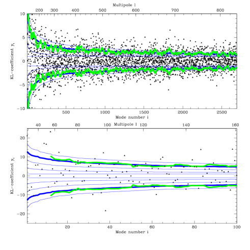
Figure 1.— The triangles show the KL-coefficients $y_{i}$ for the $21<r^{*}<22$ magnitude bin (2693 in top panel, first 100 in bottom panel). If there were no clustering in the survey, merely shot noise, they would have unit variance, and about $68\%$ of them would be expected to lie between the two horizontal lines (in the band $-1<y_{i}<1$). Cosmological fluctuations in the data would increase the standard deviation, as indicated by the other thin curves. From inside out, the thin curves correspond to the theoretically predicted rms fluctuation level $\sqrt{1+\lambda_{i}}$ with our prior power spectrum renormalized by factors 0, $(1/3)^{2}$, $(2/3)^{2}$, 1 and $(4/3)^{2}$, respectively. The green/grey curve is the rms of the data points $y_{i}$, averaged in bands of width 25, and shows the cosmological fluctuation signal rising to the left. As a rule of thumb, the $i^{th}$ KL-mode probes angular scales $\ell\sim(i/f_{\rm sky})^{1/2}\sim 16\sqrt{i}$, as indicated by upper axis labels, where $f_{\rm sky}\approx 0.004$ is the sky fraction covered in this survey (Tegmark 1997). Note that green/grey curves nearly match the power per mode predicted by the prior model curve (normalization factor 1, heavy curve), showing that this model is good for estimating errors.

2.4. Integral constraint

An important complication when computing clustering on large scales is the so-called integral constraint. Since the mean galaxy density ${\bar{n}}$ is a priori unknown, it must be estimated from the data itself, implicitly forcing the vector ${\bf x}$ to have zero mean. We tackle this problem by only using modes that are orthogonal to the (completely unknown) mean, i.e., to the vector ${\bf e}=(1,1,...,1)$ corresponding to a constant offset in the map. This idea goes back to Fisher et al. (1993) and becomes very simple to implement for our pixelized case (Tegmark et al. 1998). In principle, it suffices to add a very large noise to the mean mode, i.e., to add a huge number $M$ times ${\bf e}{\bf e}^{t}$ to the noise matrix ${\bf N}$, and the subsequent KL-compression will automatically relegate the mean mode to the list of useless ones to be discarded. In practice, we remove the mean mode analytically as described in Appendix B of Tegmark et al. (1998), which corresponds to the limit where the huge number $M\to\infty$.

2.5. Basic results

Once our data and the corresponding matrices have been KL-compressed (in which ${\bf x}$ gets replaced by ${\bf y}\equiv{{\bf B}^{\prime}}^{t}{\bf x}$, ${\bf P}_{i}$ gets replaced by ${{\bf B}^{\prime}}^{t}{\bf P}_{i}{\bf B}^{\prime}$, ${\bf N}$ gets replaced by ${{\bf B}^{\prime}}^{t}{\bf N}{\bf B}^{\prime}={\bf I}$, where the rectangular matrix ${\bf B}^{\prime}$ denotes the left part of the square matrix ${\bf B}$ corresponding to the KL column vectors we wish to keep), we proceed to compute quadratic estimators $\widehat{p}_{i}$ of our power spectrum parameters $p_{i}$. The results are shown in figures 2 and 3 and are listed in Table 1.

Since it is important for the interpretation, let us briefly review how these measurements are computed from the input data, in this case the vector ${\bf y}$ of KL-modes. A quadratic estimator $\widehat{p}_{i}$ is simply a quadratic function of the data vector, so the most general unbiased case can be written as

$$\widehat{p}_{i}\equiv{\bf y}^{t}{\bf Q}_{i}{\bf y}-s_{i},$$ (6)

where the ${\bf Q}_{i}$ are arbitrary symmetric $N\times N$-dimensional matrices and the $s_{i}\equiv\hbox{tr}\,[{\bf Q}_{i}{\bf N}]$ are the shot noise contributions. Grouping the parameters $p_{i}$ and the estimators $\widehat{p}_{i}$ into vectors denoted ${\bf p}$ and $\widehat{\bf p}$, the expected measurement is

$$\langle\widehat{\bf p}\rangle={\bf W}{\bf p}$$ (7)

for a window matrix ${\bf W}$ that can be computed from the ${\bf Q}_{i}$-matrices and the sky geometry alone (${\bf W}_{ij}=\hbox{tr}\,[{\bf P}_{i}{\bf Q}_{j}])$. The ${\bf Q}$-matrices are normalized so that each row of the window matrix sums to unity. This enables us to interpret each band power measurement $\widehat{p}_{i}$ as a weighted average of the true power spectrum $p_{j}$, the elements of the $i^{th}$ row of ${\bf W}$ giving the weights (the “window function”).

The basic idea with quadratic estimators is that each matrix ${\bf Q}_{i}$ can be chosen to effectively Fourier transform the sky map, square the Fourier modes in the $i^{th}$ power spectrum band and average the results together, thereby probing the power spectrum on that scale. We use the particular choice of ${\bf Q}$-matrices advocated by Tegmark & Hamilton (1998) (see Tegmark & Oliveira-Costa 2001 for a treatment conforming to our notation), described in Appendix A, which has the advantage of making the error bars on the measurements uncorrelated. In other words, the covariance matrix for the measured vector $\widehat{\bf p}$ is diagonal (combining shot noise and sample variance errors), so it is completely characterized by its diagonal elements, given by the error bars in Table 1 and Figure 2. This covariance matrix ${\bf M}\equiv\langle\widehat{\bf p}\widehat{\bf p}^{t}\rangle-\langle\widehat{\bf p}\rangle\langle\widehat{\bf p}\rangle^{t}$ is generally given by ${\bf M}_{ij}=2\hbox{tr}\,[{\bf Q}_{i}{\bf C}{\bf Q}_{j}{\bf C}]$ for the Gaussian case, and our particular choice of ${\bf Q}$-matrices thus reduces it to a diagonal matrix ${\bf M}_{ij}=\delta_{ij}(\Delta\widehat{p}_{i})^{2}$. ${\bf C}$ of course depends on ${\bf p}$ through equation (2), and when computing ${\bf M}$ to obtain our error bars $\Delta\widehat{p}_{i}$, we use the “prior” power spectra described below, smooth curves fitting our measurements.

The window functions corresponding to our 50 band power measurements (the rows of the matrix ${\bf W}$) are plotted in Figure 4 for the faintest magnitude bin. This connects our measurements $\widehat{p}_{i}$ to the binned underlying power spectrum $\sigma_{\ell}^{2}$. The windows are seen to have a characteristic width of order $\Delta\ell\sim 50$, which is determined by the size of our sky patch in the narrowest direction (Tegmark 1997). We are thus unable to resolve the angular power spectrum finer than this because our survey strip is so narrow in the declination direction, limiting the $\ell$-resolution to of order $\Delta\ell\sim 180^{\circ}/2.5^{\circ}$. Figure 4 also shows a notable transition around $\ell=600$. This coincides with the angular scale where the cosmological fluctuations drop below Poissonian shot noise fluctuations, and has a simple interpretation. On the larger scales where shot noise is less important, the ${\bf Q}$-matrices weight the galaxies in such a way as to make the window functions narrow, thereby minimizing the sample variance contribution to the error bars caused by power aliased from other scales. On smaller scales, the ${\bf Q}$-matrices weight all areas of the map essentially equally, without bothering with niceties such as apodization (down-weighting parts near edges), in an attempt to minimize the all-dominating shot noise. This results in less well-behaved window functions, which are both broader and are seen to have a “red leak” of power from substantially larger scales. Since the measurements beyond this transition regime are noise dominated and contain very little information, producing mere upper limits, we simply discard them. This cutoff corresponds to $\ell=$500, 500, 600 and 700 in the four magnitude bins, respectively — note that shot noise dominates the brighter magnitude bins at lower $\ell$, since they contain fewer galaxies.

To improve the signal-to-noise ratio, we average these measurements into bands as specified in Table 1. Since the original measurements are uncorrelated, so are these averages. The corresponding $14\times 50$ window function matrices for each magnitude bin, which are necessary for comparing our measurements with theoretical predictions, will be published electronically with this article and are also available at http://www.hep.upenn.edu/$\sim$max/sdss.html.

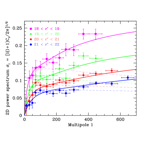
Figure 2.— The angular power spectrum $\sigma_{\ell}\equiv[\ell(\ell+1)C_{\ell}/2\pi]^{1/2}$ is shown for the four magnitude bins. The horizontal location of each point and the associated horizontal bars correspond to the mean and rms width of the corresponding window function. These measurements are uncorrelated in the approximation of Gaussian fluctuations. The curves are the “prior” power spectra used, i.e., the concordance model from Wang et al. (2001) with (solid) and without (dashed) nonlinear evolution, using four separate bias factors of order unity as described in the text.

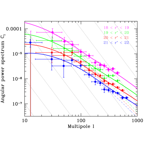
Figure 3.— Same as previous figure, but with logarithmic axes and for $C_{\ell}$ rather than $\sigma_{\ell}$. Although logarithmic axes make window functions more difficult to interpret, it facilitates connecting to the underlying 3D power spectrum $P(k)$, which is very crudely speaking the same curve shifted vertically and horizontally with different axis labels. The shifts depend on the magnitude bin: the fainter (and on average more distant) the galaxies, the further up and to the left the curve should be shifted — up because there is more averaging along the line of sight which suppresses fluctuations, to the left because a given angular scale $\ell$ corresponds to larger spatial scales. The solid lines of slope $-3$ indicate the direction of this shift when the mean survey depth is changed. In the absence of relative bias, this shifting should place the four curves on top of each other.

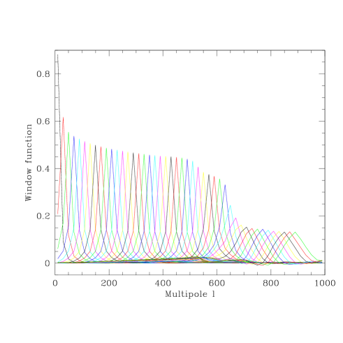
Figure 4.— Sample window functions are shown for the band-power measurements in the magnitude bin $21<r^{*}<22$. These are the rows of the window matrix ${\bf W}$, and connect our band-power measurements $\widehat{p}_{i}$ to the underlying power spectrum $\sigma_{\ell}^{2}$.

$18<r<19$		$19<r<20$		$20<r<21$		$21<r<22$
$\ell$	$\sigma_{\ell}^{2}$	$\ell$	$\sigma_{\ell}^{2}$	$\ell$	$\sigma_{\ell}^{2}$	$\ell$	$\sigma_{\ell}^{2}$
13 $\pm$ 8	-0.0006 $\pm$ 0.0028	13 $\pm$ 8	0.0002 $\pm$ 0.0011	13 $\pm$ 8	0.0004 $\pm$ 0.0005	13 $\pm$ 8	0.0008 $\pm$ 0.0003
31 $\pm$ 15	0.0115 $\pm$ 0.0048	31 $\pm$ 15	0.0053 $\pm$ 0.0021	30 $\pm$ 15	0.0017 $\pm$ 0.0010	30 $\pm$ 15	0.0009 $\pm$ 0.0006
51 $\pm$ 18	0.0132 $\pm$ 0.0059	50 $\pm$ 18	0.0067 $\pm$ 0.0028	50 $\pm$ 18	0.0034 $\pm$ 0.0015	49 $\pm$ 19	0.0013 $\pm$ 0.0008
70 $\pm$ 20	0.0185 $\pm$ 0.0064	70 $\pm$ 20	0.0105 $\pm$ 0.0031	70 $\pm$ 20	0.0088 $\pm$ 0.0017	69 $\pm$ 21	0.0043 $\pm$ 0.0010
100 $\pm$ 24	0.0192 $\pm$ 0.0048	100 $\pm$ 24	0.0128 $\pm$ 0.0024	99 $\pm$ 24	0.0075 $\pm$ 0.0013	99 $\pm$ 24	0.0052 $\pm$ 0.0008
139 $\pm$ 25	0.0261 $\pm$ 0.0052	140 $\pm$ 25	0.0107 $\pm$ 0.0025	140 $\pm$ 25	0.0069 $\pm$ 0.0014	139 $\pm$ 25	0.0045 $\pm$ 0.0009
179 $\pm$ 25	0.0229 $\pm$ 0.0056	179 $\pm$ 25	0.0133 $\pm$ 0.0027	180 $\pm$ 25	0.0079 $\pm$ 0.0015	180 $\pm$ 25	0.0039 $\pm$ 0.0010
219 $\pm$ 26	0.0272 $\pm$ 0.0061	219 $\pm$ 25	0.0179 $\pm$ 0.0028	220 $\pm$ 25	0.0103 $\pm$ 0.0015	220 $\pm$ 26	0.0052 $\pm$ 0.0010
259 $\pm$ 26	0.0357 $\pm$ 0.0067	259 $\pm$ 26	0.0114 $\pm$ 0.0030	259 $\pm$ 25	0.0087 $\pm$ 0.0016	260 $\pm$ 26	0.0040 $\pm$ 0.0010
308 $\pm$ 29	0.0353 $\pm$ 0.0060	309 $\pm$ 29	0.0205 $\pm$ 0.0027	309 $\pm$ 29	0.0098 $\pm$ 0.0014	309 $\pm$ 29	0.0054 $\pm$ 0.0009
369 $\pm$ 30	0.0544 $\pm$ 0.0067	369 $\pm$ 30	0.0291 $\pm$ 0.0030	369 $\pm$ 29	0.0133 $\pm$ 0.0015	369 $\pm$ 30	0.0067 $\pm$ 0.0009
445 $\pm$ 40	0.0545 $\pm$ 0.0066	446 $\pm$ 39	0.0268 $\pm$ 0.0027	446 $\pm$ 37	0.0144 $\pm$ 0.0013	448 $\pm$ 39	0.0086 $\pm$ 0.0008
				546 $\pm$ 37	0.0165 $\pm$ 0.0016	546 $\pm$ 38	0.0083 $\pm$ 0.0009
						646 $\pm$ 39	0.0117 $\pm$ 0.0011

Table 1. The angular power spectrum $\sigma_{\ell}^{2}\equiv[\ell(\ell+1)C_{\ell}/2\pi]$ measured for the four magnitude bins. These measurements are uncorrelated in the approximation of Gaussian fluctuations. Although the power spectrum is by definition non-negative, the allowed ranges above can include slightly negative values since our estimators are the difference of two powers (total observed power minus expected shot noise power).

2.6. Fits and priors

As mentioned above, we need to use a prior power spectrum consistent with the data to compute accurate error bars. To avoid the prior acquiring spurious wiggles caused by over-fitting noise fluctuations, it is desirable to use a smooth curve with as few tunable parameters as possible that nonetheless is consistent with the final measurements. As seen in Figure 2 and Figure 3, the simple “concordance” model from Wang et al. (2001) provides a good fit to the data in all four magnitude bins if we use bias factors $b=1.0$, $0.9$, $0.85$ and $0.8$, respectively, so we use these power spectra as priors. This is a flat neutrino-free model with purely scalar adiabatic fluctuations, a cosmological constant $\Omega_{\Lambda}=0.66$, baryon density $h^{2}\Omega_{b}=0.02$, Hubble parameter $h=0.64$ and spectral index $n_{s}=0.93$, normalized so that linear $\sigma_{8}=0.9$ for the dark matter. This model is well fit by a simple untilted BBKS power spectrum (Bardeen et al. 1986), parameterized by horizontal and vertical scaling factors $\Gamma$ and $\sigma_{8}$ as in Szalay et al. (2001), using $(\Gamma,\sigma_{8})=(0.15,0.9)$.

We have corrected for non-linear evolution using the Hamilton et al. (1991) approximation as implemented in Jain et al. (1996). Figure 2 shows nonlinear evolution to be quite important, especially for the brighter galaxies, with the corresponding linear model substantially under-predicting the power on small scales. In Section 3.2 below, we will see that the central limit theorem nonetheless produces a fairly Gaussian 2-dimensional projected galaxy distribution because of averaging along the line of sight.

We use this cosmological model merely for a convenient parametrization of our prior — physical interpretation must take into account selection function uncertainties, etc., and the reader is referred to Dodelson et al. (2001) and Szalay et al. for a detailed treatment of this. The slight differences in normalization may reflect clustering evolution, differences in bias properties between the four samples or some combination thereof.

On angular scales much smaller than a radian (the small-angle approximation), the slope $n$ of a power-law angular power spectrum $C_{\ell}$ is related to the power law slope $m$ of the angular correlation function $w(\theta)=\theta^{m}$ by $m+n=-2$, so the typical power law slopes of order $n\sim-1.5$ in Figure 3 correspond to correlation function slopes of order $m\sim-0.5$, in good agreement with the $w(\theta)$ measurement in Connolly (2001).

2.7. Relation to 3D power spectrum

Let us conclude this section by briefly commenting on how to interpret our measurements. In a companion paper (Dodelson et al. 2001), the present results and those on the angular correlation function from S2001 are used to recover an estimated 3D power spectrum $P(k)$. Here we present the relevant window functions that are used as a starting point for such analyses.

As described by Huterer et al. (2001) and Appendix B, the angular power spectrum $C_{\ell}$ is related to the 3D power spectrum $P(k)$ via the simple relation

$$C_{\ell}={2\over\pi}\int_{0}^{\infty}f_{\ell}(k)^{2}P(k)k^{2}dk,$$ (8)

where the dimensionless function

$$f_{\ell}(k)\equiv\int_{0}^{\infty}j_{\ell}(kr)f(r)dr.$$ (9)

Here $f$ is the probability distribution for the comoving distance $r$ to a random galaxy in the survey, optionally weighted by an evolution factor, and $j_{\ell}$ is a spherical Bessel function. In other words, the integral kernel transforming from 3D to our angular 2D case is simply a Bessel-transform of the radial selection function. A sample of these integral kernels are plotted in Figure 5. Accurate approximations of this kernel are available in the small-angle limit, but we use the full expression here since it is so simple (computational details are given in Appendix B), and since scales where sky-curvature is non-negligible will eventually be well probed by the SDSS.

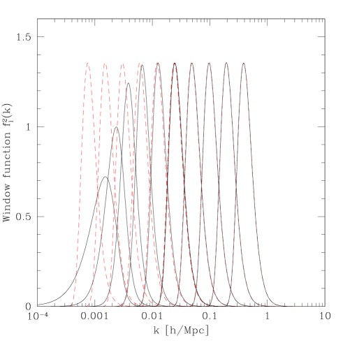
Figure 5.— The solid curves show the exact $k$-space window function corresponding to $C_{\ell}$ for multipoles $\ell=1$, 2, 4, 8, 16, 32, 64, 128, 256 and 512, respectively, renormalized to have unit area, using the radial selection function for magnitude bin $21<r<22$. The dashed curves show the same window functions computed in the small-angle approximation. These window functions connect the angular power spectrum $C_{\ell}$ to the underlying 3D power spectrum $P(k)$ via equation (8).

By taking linear combinations of the kernels from Figure 5 corresponding to our $\ell$-space window functions, we obtain the kernels of Figure 6, showing which $k$-values each of our band-power measurements is probing. This enables us to interpret our band-powers as measuring weighted averages of the 3D power spectrum $P(k)$ as shown in Figure 7. This plot is by no means a substitute for a thorough reconstruction of the 3D power spectrum as in Dodelson et al. (2001), incorporating selection function uncertainties etc, but provides a useful rough guide as to which spatial scales are probed and, in particular, as to the $\ell$-values for each magnitude bin beyond which nonlinear clustering is likely to be important.

To gain further intuition about the relation between $C_{\ell}$ and $P(k)$, an additional approximation is instructive. As shown in Appendix B, the 2D and 3D power spectra are approximately related by

$$C_{\ell}\approx{\alpha\over r_{*}^{3}}P(k),$$ (10)

where $k=\beta\ell/r_{*}$ and $r_{*}$ is the mean spatial depth of the survey. The key approximation made here is that $C_{\ell}$ in fact probes not simply the power $P$ at wavenumber $k$, but rather a weighted average of $P$ with a window function of width $\Delta k\approx\gamma k$. Here $\alpha$, $\beta$ and $\gamma$ are dimensionless constants of order unity that depend only on the shape of the radial selection function, not on its depth. For the SDSS case described in Dodelson et al. (2001), $\alpha\approx 0.75$, $\beta\approx 1.1$ and the smoothing width $\gamma=\Delta k/k\approx 0.37$.

In other words, we can interpret $C_{\ell}$ as a smoothed version of $P(k)$ shifted vertically and horizontally in a log-log plot such as Figure 3. Moreover, equation (10) shows that mis-estimates of the radial selection function depth $r_{*}$ will simply shift the entire $P(k)$-curve along the lines of slope $-3$ shown in Figure 7, without changing its shape.

Figure 6.— The curves show the $k$-values probed by our 14 band power measurements for the faintest magnitude bin, thereby connecting what we measure to the 3D power spectrum $P(k)$. In other words, these window functions, defined by equation (B23), are analogous to those in Figure 4, but in $k$-space rather than $\ell$-space.

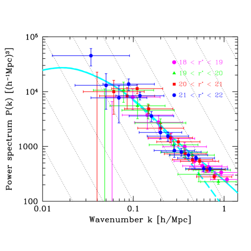
Figure 7.— The same band power measurements as in Figure 2, but plotted in $k$-space using the window functions from Figure 6. Specifically, the data points are the rescaled band power coefficients which probe a weighted average of $P(k)$ as specified by equation (B23). An inversion from 2D to 3D power spectra is performed in Dodelson et al. (2001) — the data plotted here are merely the input to those calculations. For comparison, the solid curve is the $\Lambda$CDM “concordance” model from Wang et al. (2001) with (solid) and without (dashed) nonlinear evolution. If the mean depth has been underestimated for one of the Galaxy samples, the corresponding points should shift up to the left along the dotted lines of slope $-3$.

3. Robustness and limitations of results

How reliable are the angular power spectrum measurements computed above? In this section, we discuss the underlying assumptions and their limitations. We focus on three areas and discuss them in turn: potential problems with the input data, potential problems with the data processing (analysis algorithms/software) and potential problems with underlying assumptions, notably Gaussianity.

3.1. Issues related to the input data

The input data used in our analysis have been extensively tested for potential systematic errors by S2001, and constitute arguably the cleanest deep angular survey data to date. In particular, S2001 present a battery of tests for problems involving star-galaxy separation and modulation of the galaxy detection efficiency by external effects such as photometric calibration, seeing conditions and Galactic extinction. By cross-correlating the galaxy maps with various two-dimensional “trouble templates” corresponding to variations in seeing, reddening, stellar density, camera column structure, etc., the various effects were quantified and reduced to negligible levels by sharpening the seeing and reddening cuts. This gives us confidence that the errors in our star-galaxy separation algorithm (which depends on seeing) and reddening estimates have negligible effect on our estimates of angular power spectra even in the faintest magnitude bin.

As an additional precaution, we complement the tests from S2001 with three that are tailored for our $C_{\ell}$-analysis. Specifically, we compute the angular power spectra of the seeing and reddening templates, which were found to be the most serious challenges in S2001, and with a photometric calibration error template. Strictly speaking, these of course do not have well-defined power spectra, since they are not isotropic random fields. Rather, what is relevant here is the amplitude and shape of the bias that they would add to our estimates of the galaxy power spectra. We therefore process these templates in exactly the same way as the galaxy maps, with the pair-weightings (the ${\bf Q}_{i}$-matrices) given by the galaxy noise and signal matrices. We use the weighting and sky mask corresponding to the faintest magnitude bin, since this is the one that is most vulnerable to these systematics — both because these galaxies have the poorest signal-to-noise ratio in the CCD photometry (Lupton et al. 2001) and because they have the lowest intrinsic angular clustering amplitude.

We use the same seeing and reddening templates as S2001, i.e., the second moment of the point-spread function for each pixel and the extinction correction from Schlegel et al. (1998). In order to provide a meaningful comparison between the amplitudes of signal and systematics, we need to estimate the conversion factor from seeing or reddening power to galaxy fluctuation power. We do this using the cross-correlations presented in figures 8 and 9 of S2001. To be conservative and err on the side of caution, we use the relevant $2\sigma$ cross-correlation upper limits, 0.0017 and 0.0038, for seeing and reddening, respectively. These values are the largest upper limit on any angular scale, but we have used them at all angular scales $\ell$ to be conservative.

The corresponding angular power spectra for seeing and extinction are shown in Figure 8 and, as opposed to the galaxy fluctuations, they are seen be flat or rise towards larger angular scales. For the reddening case, this is in good agreement with the findings of Vogeley (1998) and measurements of the dust power spectrum. The combined DIRBE and IRAS dust maps suggest a power law $C_{\ell}\propto\ell^{-2.5}$ (Schlegel et al. 1998), and a recent analysis of the DIRBE maps has supported an even redder slope with an $\ell^{-3}$ power law for $\ell\mathrel{\hbox to0.0pt{\lower 3.0pt\hbox{$\mathchar 536\relax$}\hss}\raise 2.0pt\hbox{$\mathchar 316\relax$}}300$ (Wright 1998).

As a template for photometric calibration errors, we identify a feature of the stellar distribution in color space and measure it as a function of position in the sky. As seen, e.g., in Finlator et al. (2000), the locus of stars in the $g-r,r-i$ color plane shows two branches: stars cooler than $\sim$M0 have almost constant $g-r$ colors, while hotter stars show a strong correlation between the $g-r$ and $r-i$ color. The crossing point of linear fits to the stellar locus in these two branches should be independent of position on the sky, thus variations in this crossing point are a sensitive measure of photometric calibration errors in $g,r$ and $i$. Similarly, the stellar locus in the $r-i,i-z$ plane is almost linear; one can define the $i-z$ color corresponding to the $r-i$ color of the crossing point measured from the $g-r,r-i$ plane.

We have measured the crossing colors from the stars in our sample on scales of two degrees by 13 arcminute (the width of a scanline), and attribute all observed variations to errors in $r^{*}$ to be conservative; the distribution of the implied error is roughly Gaussian, with a sigma of 0.015 magnitudes. We convert these $r^{*}$-fluctuations into density fluctuations by multiplying by the source count slope $d\,\hbox{ln}\,N/dr$. This slope is of order unity at $r^{*}=19$ and flattens at fainter magnitudes (Yasuda et al. 2001), so we make the conservative assumption $d\,\hbox{ln}\,N/dr=1$. The angular power spectra of these two calibration error maps are shown in Figure 8 and are seen to be approximately flat (scale-invariant).

the almost horizontal part towards the left, and stars later than $\sim$M0 are found in the vertical branch with $g^{\prime}-r^{\prime}\sim 1.4$

It is reassuring that even with the extremely pessimistic assumptions described above, the expected contaminant signals remain much smaller than the observed galaxy power spectrum all the way out to the largest scales currently probed. Extrapolation to extremely large scales suggests that even extinction should remain subdominant for $\ell\mathrel{\hbox to0.0pt{\lower 3.0pt\hbox{$\mathchar 536\relax$}\hss}\raise 2.0pt\hbox{$\mathchar 318\relax$}}5-10$.

In summary, we have found that systematics are small even in the nearly worst-case scenario shown in Figure 8. Moreover, the SDSS will provide other internal checks on many systematics, notably the extinction correction, so these are unlikely to prove a significant limitation on determining the power spectrum.

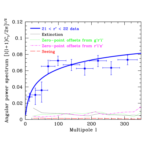
Figure 8.— To give a feeling for the magnitude of potential systematic errors, the power spectrum in the faintest (and most vulnerable) magnitude bin is compared with the power spectra for seeing, extinction and photometry related modulations of the observed galaxy density under very pessimistic assumptions.

3.2. Issues related to algorithms, software and assumptions

Since our analysis consists of a number of somewhat complicated steps, it is important to test the integrity of both the software and the underlying methods. We do this using two types of Monte Carlo simulations:

1. We analyze 1000 Monte-Carlo maps ${\bf x}$ that are drawn from a multivariate Gaussian distribution with vanishing mean and covariance matrix ${\bf C}$.

2. We analyze 100 Monte-Carlo galaxy samples including non-linear clustering as described in Scoccimarro & Sheth (2001) and S2001.

Both sets of mock data were processed through our analysis pipeline, enabling us to check not only whether we obtained the correct answer on average, but also whether the scatter and the error correlations corresponded to the predicted values. The first suite of Monte Carlos offered precision end-to-end tests of the algorithms and the software, since errors or bugs in any of the many intermediate steps would have manifested themselves here. They used the exact same survey geometry as the real data, including the seeing and reddening masks of S2001.

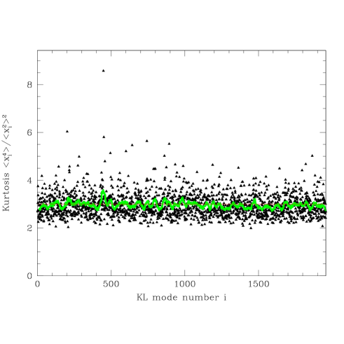
Figure 9.— The simulated kurtosis of the first 1957 KL-coefficients is shown for the $18<r<19$ magnitude bin. Each triangle represents the kurtosis of the distribution for the corresponding mode as measured from the 100 nonlinear Monte Carlo simulations described in the text. The thick curve shows a running average of 25 modes, whereas the thin horizontal line shows the Gaussian prediction of three.

The second suite of Monte Carlos provides a way of quantifying the limits of applicability of the Gaussian assumption. They were constructed using the PTHalos code (Scoccimarro & Sheth 2001) as described in detail in Scranton et al (2001), covering a rectangular $90^{\circ}\times 2.5^{\circ}$ sky region. In short, this code is a fast approximate method to build non-Gaussian density fields with realistic correlation functions, including non-trivial galaxy biasing (obtained by placing galaxies within dark matter halos with a prescribed halo occupation number as a function of halo mass).

The non-Gaussian effects produced by non-linear evolution encode information that can be captured by measuring higher-order moments and other statistics. Since this route is explored in detail in Szapudi et al. (2001), we will not pursue it here. However, we need to quantify the level to which this non-Gaussianity affects our results.

Since our power spectrum estimates are simply quadratic functions of the density field, they give unbiased measurements of the underlying power spectrum even if the fluctuations are non-Gaussian. In other words, our calculation of window functions, KL-modes etc. is completely general and does not make any assumptions about Gaussianity. The one place in the quadratic estimator formalism where Gaussianity is assumed is in the computation of error bars. Since the variances of our power spectrum estimates involve fourth moments of the observed density fields (kurtosis), they will generally differ from the Gaussian prediction in the presence of non-Gaussianity — typically by being larger. The covariance between band power estimates likewise involves fourth moments, so we should not expect our error bars to retain their attractive property of being uncorrelated down into the nonlinear regime. The third moment (skewness) of the galaxy distribution also affects the power spectrum error bars via coupling to the Poissonian shot noise, at a level of the same order of magnitude as the kurtosis.

To quantify this effect, Figure 9 shows the kurtosis of the first 1957 KL-coefficients for the $18<r<19$ magnitude bin. (This brightest magnitude bin is expected to be the most non-Gaussian, both because it probes the smallest spatial scales and because it involves the least amount of line-of-sight averaging — such averaging makes the density field mory Gaussian as per the central limit theorem .) The kurtosis was computed by processing the 100 nonlinear Monte Carlo simulations through our analysis pipeline and computing the variance and fourth moment of the 100 values obtained for each mode. The dimensionless kurtosis plotted is the fourth moment divided by the square of the variance, i.e., $\langle y_{i}^{4}\rangle/\langle y_{i}^{2}\rangle^{2}$, and would equal three for Gaussian fluctuations (in which case the KL-coefficients would be simply independent Gaussian random variables). Since we have only 100 simulations, there is still a fair amount of scatter. To further reduce the scatter, we have therefore added a line in Figure 9 showing a running average of 25 consecutive triangles. The scatter (which is determined by eighth moments) appears to rise somewhat initially, as modes probe progressively smaller angular scales, then decreases again as cosmological fluctuations become smaller than Poisson shot noise fluctuations. However, the kurtosis itself, which (with the skewness) is the only quantity that affects our error bars, is seen not to depart significantly from the Gaussian value on any of the angular scales we have probed. This implies that non-Gaussianity does not appear to have a major impact on our results. This is partly by design, since we chose to focus our analysis on the largest scales.

In other words, although non-Gaussian effects are very strong on small scales (indeed, the onset of non-linear evolution is evident in Figure 2), they have only a weak effect on the error bars of our large scale angular power spectrum. Factors contributing to this are the dominance of shot noise on small scales (on a mode-by-mode basis) as well as the central limit theorem, suppressing non-Gaussianity by averaging fluctuations along the line of sight.

In conclusion, we have computed the large-scale angular power spectrum from early SDSS data and performed a series of tests validating our results. The cosmological implications of our measurements are discussed in a companion paper by Dodelson et al. (2001). Although these results are interesting in their own right, perhaps the most important conclusion is that the lack of discernible systematic errors even on scales as large as tens of degrees bodes extremely well for analysis of future SDSS data. The present data covered about 160 square degrees, i.e., less than $2\%$ of the full survey that will eventually be available, so angular clustering studies are likely to remain at the forefront of the quest for a detailed understanding of cosmic clustering.

The authors wish to thank Andrew Hamilton and Lloyd Knox for helpful comments.

The Sloan Digital Sky Survey (SDSS) is a joint project of The University of Chicago, Fermilab, the Institute for Advanced Study, the Japan Participation Group, The Johns Hopkins University, the Max-Planck-Institute for Astronomy (MPIA), the Max-Planck-Institute for Astrophysics (MPA), New Mexico State University, Princeton University, the United States Naval Observatory, and the University of Washington. Apache Point Observatory, site of the SDSS telescopes, is operated by the Astrophysical Research Consortium (ARC).

Funding for the project has been provided by the Alfred P. Sloan Foundation, the SDSS member institutions, the National Aeronautics and Space Administration, the National Science Foundation, the U.S. Department of Energy, the Japanese Monbukagakusho, and the Max Planck Society. The SDSS Web site is http://www.sdss.org/. MT was supported by NSF grant AST00-71213, NASA grants NAG5-9194 and NAG5-11099, the University of Pennsylvania Research Foundation and the David and Lucile Packard Foundation. SD is supported by the DOE and by NASA grant NAG5-7092 at Fermilab, and by NSF Grant PHY-0079251. DJE was supported by NASA through Hubble Fellowship grant #HF-01118.01-99A from the Space Telescope Science Institute, operated by the AURA Inc., under NASA contract NAS5-26555.

A. The relation between

DIFFERENT QUADRATIC ESTIMATORS

The purpose of this Appendix is to describe the ${\bf Q}$-matrices that define our analysis as well as to elucidate the relationship between quadratic estimators of $C_{\ell}$, $w(\theta)$ and $P(k)$. From an information-theoretic point of view, we will see that the key issue is not which of the three functions one tries to measure, but what pair weighting is used in the process — the minimum-variance weighting retains all information about all three of them in the Gaussian approximation. Indeed, we will see that the decorrelated minimum-variance estimators of all three functions are one and the same set of numbers, just normalized differently!

A.1. The ${\bf Q}$-matrices used in our analysis

As described in Section 2.5, our power spectrum estimators are quadratic functions of the observed galaxy density. The estimator of the power in the $i^{th}$ band is therefore defined by a symmetric matrix ${\bf Q}_{i}$ that gives the weight assigned to each pair of pixels (or KL-coefficients) via equation (6). In our analysis, we make the choice

$${\bf Q}_{i}=\sum_{j}({\bf B})_{ij}{\bf C}^{-1}{\bf P}_{j}{\bf C}^{-1}$$ (A1)

for a $50\times 50$ matrix ${\bf B}$ that will be defined below. It can be shown (Tegmark 1997) that this choice distills all the cosmological information from the original galaxy map ${\bf x}$ into the (much shorter) vector $\widehat{\bf p}$ in the approximation of Gaussian fluctuations, as long as the matrix ${\bf B}$ is invertible and the binning scale $\Delta\ell$ is narrower than the scale on which the power spectrum varies substantially. In this approximation, the mean and covariance of the quadratic estimator vector $\widehat{\bf p}$ defined by equation (6) is given by

$$\langle\widehat{\bf p}\rangle = {\bf B}{\bf F}{\bf p},$$ (A2)

$${\bf M}\equiv\langle\widehat{\bf p}\widehat{\bf p}^{t}\rangle-\langle\widehat{\bf p}\rangle\langle\widehat{\bf p}\rangle^{t} = {\bf B}{\bf F}{\bf B}^{t},$$ (A3)

where

$${\bf F}_{ij}={1\over 2}\hbox{tr}\,\left[{\bf C}^{-1}{\bf P}_{i}{\bf C}^{-1}{\bf P}_{j}\right]$$ (A4)

is the so-called Fisher information matrix. As advocated in Tegmark & Hamilton (1998), we choose ${\bf B}={\bf D}{\bf F}^{-1/2}$, where ${\bf D}$ is a diagonal matrix whose elements are chosen so that the window matrix ${\bf W}={\bf B}{\bf F}$ has unit row sums. This choice has the virtue of giving uncorrelated error bars (the covariance matrix of equation (A3) becomes the diagonal matrix ${\bf M}={\bf D}^{2}$) and narrow, well-behaved window functions as seen in Figure 4.

A.2. The relation between quadratic estimators of $C_{\ell}$, $w(\theta)$ and $P(k)$

Suppose the angular power spectrum parameters $p_{i}$ can be expressed as linear combinations of some other parameters $p^{\prime}_{i}$, i.e.,

$${\bf p}={\bf A}{\bf p}^{\prime}$$ (A5)

for some matrix ${\bf A}$. There are two such interesting examples, involving $w(\theta)$ and $P(k)$, respectively. If we define $p^{\prime}_{i}\equiv w(\theta_{i})$, i.e., the angular correlation function amplitude in the $i^{th}$ angular bin, then ${\bf A}$ is given by

$${\bf A}_{\ell i}={1\over 2\pi}P_{\ell}(\cos\theta_{i})\sin\theta_{i}\Delta\theta,$$ (A6)

where $P_{\ell}$ is a Legendre polynomial and $\Delta\theta$ is the width of the angular bins. If we define $p^{\prime}_{i}\equiv P(k_{i})$, i.e., the 3D power spectrum in the $i^{th}$ $k$-bin, then ${\bf A}$ is given by

$${\bf A}_{\ell i}=K_{\ell}(k_{i})k_{i}^{3}\Delta\,\hbox{ln}\,k,$$ (A7)

where $K_{\ell}$ is given by equation (B14) and $\Delta\,\hbox{ln}\,k$ is the width of the (logarithmic) $k$-bins. (Throughout this subsection, we assume for simplicity the $\theta$- or $k$-bins are narrow enough to resolve any features in $w(\theta)$ or $P(k)$, and that there is no $\ell$-binning, defining $p_{\ell}=C_{\ell}$.)

Using equation (A5), we can construct quadratic estimators $\widehat{\bf p}^{\prime}$ to measure ${\bf p}^{\prime}$ directly, without going through the intermediate step of measuring the angular power spectrum ${\bf p}$ first. Writing ${\bf S}=\sum p^{\prime}_{i}P^{\prime}_{i}$ by analogy with equation (2), the new ${\bf P}$-matrices are given in terms of the old ones by

$${\bf P}^{\prime}_{i}=\sum_{j}{\bf A}^{t}_{ij}{\bf P}_{j}.$$ (A8)

Using equations (6) and (A1) therefore shows that the new estimators are related to the old ones by

$$\widehat{\bf p}^{\prime}={\bf B}^{\prime}{\bf A}^{t}{\bf B}^{-1}\widehat{\bf p}.$$ (A9)

Here ${\bf B}^{\prime}$ is the ${\bf B}$-matrix corresponding to the new parameters ${\bf p}^{\prime}$, and we use the same notation with primes ^′ for other matrices below. To obtain an intuitive understanding for this relation, let us simplify things by using the choice ${\bf B}\equiv{\bf D}{\bf L}^{-1}$ in place of our previous choice ${\bf B}\equiv{\bf D}{\bf F}^{-1/2}$, where ${\bf L}$ is the lower-triangular matrix obtained by Cholesky-decomposing the Fisher matrix as ${\bf F}={\bf L}{\bf L}^{t}$. ${\bf L}$ can be viewed of as simply an alternate choice of square root of ${\bf F}$. As described in Tegmark & Hamilton (1998), this choice has the same desirable properties as ${\bf B}\equiv{\bf D}{\bf F}^{-1/2}$ except that it gives asymmetric window functions (${\bf F}^{1/2}$ is symmetric whereas ${\bf L}$ is not). A straightforward calculation shows that ${\bf F}^{\prime}={\bf A}^{t}{\bf F}{\bf A}$, so ${\bf L}^{\prime}={\bf A}^{t}{\bf L}$ and equation (A9) reduces to

$$\widehat{\bf p}^{\prime} = ({\bf D}^{\prime}{{\bf L}^{\prime}}^{-1}){\bf A}^{t}({\bf D}{\bf L}^{-1})^{-1}{\bf p}$$ (A10)

$$= ({\bf D}^{\prime}{\bf L}^{-1}{\bf A}^{t}){\bf A}^{t}({\bf L}{\bf D}^{-1}){\bf p}={\bf D}^{\prime}{\bf D}^{-1}{\bf p},$$

a diagonal matrix. In other words, if we use the same number of $\ell$-values as there are bins (for $\theta$ or $k$), with ${\bf A}$ an invertible square matrix, then the old estimators $\widehat{p}_{i}$ and the new estimators $\widehat{p}^{\prime}_{i}$ are the exact same numbers except differently normalized! The normalization factors ${\bf D}_{ii}$ and ${\bf D}^{\prime}_{ii}$ simply let us interpret the measurements as probing weighted averages of ${\bf p}$ and ${\bf p}^{\prime}$, respectively.

This shows that there is no fundamental difference between measuring $C_{\ell}$, $w(\theta)$, $P(k)$ or some other linear transformation of the power spectrum with quadratic estimators of the form of equation (A1). Not only do they all contain the same information (keeping the ${\bf P}$-matrices the same, two different $\widehat{\bf p}$ computed with different ${\bf B}$-matrices are trivially related by $\widehat{\bf p}^{\prime}={\bf B}^{\prime}{\bf B}^{-1}\widehat{\bf p}$), but even the ${\bf B}$-matrices will be essentially the same if we decorrelate the measurements. This means that the rescaled $C_{\ell}$-estimates shown in Figure 7 can alternatively be interpreted as decorrelated quadratic estimators of $P(k)$, or as rescaled decorrelated quadratic estimators of $w(\theta)$! The reason that this paper purports to measure $C_{\ell}$ rather than $w(\theta)$ is simply that the window-functions for our estimators turn out to be narrow and well-behaved in $\ell$-space, but wide and partially negative in $\theta$-space.

A.3. The relation between different pair weightings

In the companion paper by Connolly et al. (2001), the angular correlation function $w(\theta)$ was measured with a different technique, using so-called Landy-Szalay (LS) estimators. LS-estimators are also quadratic estimators, and in our notation corresponds to replacing the ${\bf Q}$-matrix choice of equation (A1) by

$${\bf Q}_{i}=N_{i}{\bf P}_{i}.$$ (A11)

For the $w(\theta)$-case, the ${\bf P}$-matrices take the simple form ${\bf P}_{jk}=1$ if the angular separation between pixels $j$ and $k$ falls in the angular bin around $\theta_{k}$, vanishing otherwise. The normalization constants $N_{i}$ are simply the number of pixel pairs with angular separation in the $i^{th}$ angular bin, so $N_{i}=\hbox{tr}\,{\bf P}_{i}^{2}$. The estimators corresponding to equation (A11) are not simply related to those corresponding to equation (A1) since the ${\bf C}^{-1}$-weighting is absent. They therefore do not contain the same cosmological information. However, they have two other very desirable properties. The first is that the window matrix from equation (7) is

$${\bf W}_{ij}\equiv\hbox{tr}\,[{\bf P}_{i}{\bf Q}_{j}]=N_{i}\hbox{tr}\,[{\bf P}_{i}{\bf P}_{j}]=\delta_{ij},$$ (A12)

the identity matrix. This means that the LS quadratic estimators can be interpreted as exact measurements of $w(\theta)$ with no smoothing whatsoever. The second advantage is computational speed. Since no time-consuming matrix inversions are necessary, the LS-estimator of $w(\theta)$ can be computed with many more pixels than would otherwise be feasible, probing the clustering down to far smaller angular scales than we have probed in this paper. Finally, it is worth noting that the lossless property of the quadratic estimators of equation (A1) breaks down on small scales where fluctuations become non-Gaussian, making the computationally superior LS-estimators preferable in this regime. The bottom line is that the $C_{\ell}$-estimation used here and the LS-estimation of $w(\theta)$ used in Connolly et al. (2001) are highly complementary approaches, being preferable on large and small angular scales, respectively.

B. The relation between $C_{\ell}$ and $P(k)$

In this Appendix, we discuss the close relation between the angular power spectrum $C_{\ell}$ that we have measured and the underlying 3D power spectrum $P(k)$. The purpose is both to review their exact quantitative relation, and to provide qualitative intuition for this relation and how it is affected by mis-estimates of the radial selection function. As we will see, $C_{\ell}$ can be interpreted as essentially a smoothed version of $P(k)$ shifted horizontally and vertically on a log-log plot, and a mis-estimate of the mean survey depth would shift the power spectrum along lines of slope $-3$.

B.1. The exact relation

The angular power spectrum $C_{\ell}$ is related to the 3D power spectrum $P(k)$ by

$$C_{\ell}=\int_{0}^{\infty}K_{\ell}(k)P(k)k^{2}dk$$ (B13)

for a dimensionless integral kernel $K_{\ell}(k)$ that depends on the radial selection function of the survey. As shown in Appendix A of Huterer et al. (2001),

$$K_{\ell}(k)={2\over\pi}f_{\ell}(k)^{2},$$ (B14)

where $f_{\ell}$ is the Bessel transform of the radial selection function $f(r)$ as given by equation (9). Specifically, $f(r)=g(r)h(r)$, where $g(r)$ is the probability distribution for the comoving distance from us to a random galaxy in the survey and $h(r)$ is an optional (bias and clustering) evolution term of order unity, so $g$ has units of inverse length and $h$ is dimensionless. Defining ${N}$ to be the expected number of galaxies within a sphere of a certain radius, we thus have

$$g(r)\propto{d{N}\over dr}={d{N}/dz\over dr/dz}={H(z)\over H_{0}r_{0}}{d{N}\over dz},$$ (B15)

normalized so that

$$\int_{0}^{\infty}g(r)dr=1.$$ (B16)

Here $r_{0}\equiv c/H_{0}\approx 3000h^{-1}$Mpc, and the relative Hubble parameter is

$${H(z)\over H_{0}}=\sqrt{\Omega_{\Lambda}+(1-\Omega_{\Lambda}-\Omega_{m})(1+z)^{2}+\Omega_{m}(1+z)^{3}}$$ (B17)

for a cosmology with density parameters $\Omega_{m}$ and $\Omega_{\Lambda}$ for matter and vacuum energy, respectively. This means that uncertainties about $d{N}/dz$ and uncertainties about the cosmological parameters $(\Omega_{m},\Omega_{\Lambda})$ get combined, entering only via the single function $g(r)$.

The evolution term $h(r)$ relates the past and present galaxy clustering amplitudes, and is given by

$$h=[P(k;z)/P(k)]^{1/2}$$ (B18)

for a flat Universe. If space should turn out to be curved despite present evidence to the contrary, $h$ gets multiplied by a correction factor as in Peebles (1980). The factor $h$ is likely to remain close to unity for the low redshifts $z\mathrel{\hbox to0.0pt{\lower 3.0pt\hbox{$\mathchar 536\relax$}\hss}\raise 2.0pt\hbox{$\mathchar 316\relax$}}0.5$ probed by the SDSS, especially since the effects of bias evolution and dark matter clustering evolution appear to partially cancel (Blanton et al. 2000). The clustering evolution is expected to be small over this redshift range since linear growth grinds to a halt at recent times when vacuum energy becomes dominant. Rather than attempting a complicated and poorly justified model for $h(r)$, we therefore simply set $h(r)=1$ and reinterpret the measured $P(k)$ as the power spectrum at the effective redshift corresponding to $r\sim\ell/k$ (Dodelson et al. 2001).

In practice, we evaluate the Bessel-transform of equation (9) for 512 logarithmically equispaced $k$- and $r$-values using Fourier methods from the FFTlog package of Hamilton (2000). This is an efficient $N\,$log$\,N$ algorithm, evaluating all kernels up to $\ell=1000$ in about a minute on a workstation. Sample results are shown in Figure 5 using the selection function for the $21<r<22$ band described by Dodelson et al. (2001) for a Universe with $\Omega_{m}=0.3$, $\Omega_{\Lambda}=0.7$.

B.2. The small-angle approximation

The approximation

$$K_{\ell}(k)\approx{1\over\ell k^{2}}f\left({\ell\over k}\right)^{2},$$ (B19)

becomes accurate in the small-angle limit (see, e.g., Kaiser 1992; Baugh & Efstathiou 1994), as illustrated in Figure 5. This is the $\ell$-space version of Limber’s equation, which relates $P(k)$ to the angular correlation function $w(\theta)$. Equation (B19) can be derived directly from equation (B14) by noting that for large $\ell$, the spherical Bessel function $j_{\ell}(kr)$ becomes sharply peaked around $kr=\ell$. Assuming that $f(r)$ is a smoothly varying function relative to this peak width, we can thus approximate it by $f(\ell/k)$ and take it out of the integral in equation (9), obtaining

$$f_{\ell}(k)\approx f\left({\ell\over k}\right)\int_{0}^{\infty}j_{\ell}(kr)dr\approx\left({\pi\over 2k^{2}\ell}\right)^{1/2}f\left({\ell\over k}\right),$$ (B20)

since

$$\int_{0}^{\infty}j_{\ell}(x)dx={\sqrt{\pi}\over 2}{\Gamma\left({\ell+1\over 2}\right)\over\Gamma\left({\ell+2\over 2}\right)}\approx\sqrt{\pi\over 2\ell}$$ (B21)

for $\ell\gg 1$.

B.3. $k$-space window functions

Since our measured band powers probe linear combinations of the actual power spectrum coefficients $C_{\ell}$, and these in turn are linear combinations of $P(k)$, we can reinterpret our band-power measurements $\widehat{p}_{i}$ as probing $P(k)$ directly. In other words, the window matrix ${\bf W}$ from equation (7) relates our measurements to $C_{\ell}$ and the kernel $K_{\ell}(k)$ of equation (B13) relates $C_{\ell}$ to $P(k)$, so combining the two relates our measurements to $P(k)$. Specifically, these two equations give

$$\langle\widehat{p}_{i}\rangle=\int_{0}^{\infty}\sum_{\ell}W_{i\ell}K_{\ell}(k)P(k)k^{2}dk$$ (B22)

for the case of no $\ell$-binning. Since we have binned our angular power spectrum in $\ell$-bins of width $\Delta\ell=20$, the sum over $\ell$ in equation (B22) gets replaced by a sum over bins and $K_{\ell}(k)$ gets replaced by its average over each $\ell$-bin.

Equation (B22) is seen to take the simple form $\langle\widehat{p}_{i}\rangle=\int W_{i}(k)P(k)d\,\hbox{ln}\,k$ for functions $W_{i}(k)\equiv\sum_{\ell}W_{i\ell}K_{\ell}(k)k^{3}$ that are never negative. Defining normalization constants $c_{i}\equiv\int W_{i}(k)d\,\hbox{ln}\,k$, this means that we can interpret our measurements $\widehat{p}_{i}$ as probing simply $c_{i}$ times weighted averages of $P(k)$ with weight functions $W_{i}(k)/c_{i}$. However, caution is necessary before using this fact to make plots like Figure 7. The reason is that if the window functions $W_{i}(k)/c_{i}$ are wide (which they are) and the function to be measured varies substantially on the scale of this window (which $P(k)$ typically does), then the weighted average will be dominated by one edge of the window. For instance, in the regime of Figure 7 where $P(k)$ is rapidly falling, the integral $\int W_{i}(k)P(k)d\,\hbox{ln}\,k$ would be dominated by the contribution from $k$-values leftward of the peak of $W_{i}(k)$, causing the corresponding point in Figure 7 to be plotted misleadingly far to the right. Such problems can be avoided by redefining the quantity to be measured to be a roughly constant function. This is why we chose to measure $\sigma_{\ell}^{2}$ rather than $C_{\ell}$ above. Following, e.g., Eisenstein & Zaldarriaga (2000) and Hamilton et al. (2000), we therefore interpret our measurements as weighted averages of the relative power spectrum, defined as $P(k)/P_{*}(k)$, where $P_{*}(k)$ is our fiducial power spectrum described in Section 2.5. This relative power will be a fairly constant function (of order unity) as long as the shape of our fiducial power spectrum is not grossly inconsistent with the truth. We therefore write

$$\langle\widehat{p}_{i}\rangle=\int W_{i}(k){P(k)\over P_{*}(k)}d\,\hbox{ln}\,k,$$ (B23)

where we have defined window functions

$$W_{i}(k)\equiv P_{*}(k)k^{3}\sum_{\ell}W_{i\ell}K_{\ell}(k),$$ (B24)

These functions are plotted in Figure 6 for the faintest magnitude bin. This equation is analogous to equation (7), linking our measurements to the 3D power spectrum $P(k)$ rather than the angular spectrum $C_{\ell}$. The rescaled band-power coefficients $\widehat{p}_{i}/c_{i}$ are thus weighted averages of the relative power spectrum, where $c_{i}\equiv\int W_{i}(k)d\,\hbox{ln}\,k$ as before. The numbers $(P_{*}(k)/c_{i})\widehat{p}_{i}$ can therefore be viewed as a measurements of $P(k)$, and are plotted in Figure 7 at the $k$-values corresponding to the means of the distributions $W_{i}(k)$, with horizontal bars indicating the rms widths of $W_{i}(k)$. The results are seen to be roughly consistent between magnitude bins and in agreement with a standard $\Lambda$CDM power spectrum.

B.4. The narrow window approximation and the poor man’s Limber inversion

Let us now make an approximation aimed at building qualitative intuition for how $C_{\ell}$ is related to $P(k)$ and, in particular, for how this relation depends on the details of the selection function $f(r)$. Figure 5 shows that the kernels $K_{\ell}(k)$ from equation (B13) are fairly narrow positive functions with a single peak. Defining their $n^{\rm th}$ moments as

$$\langle k^{n}\rangle_{\ell}\equiv\int K_{\ell}(k)k^{n}d\,\hbox{ln}\,k,$$ (B25)

they are therefore roughly characterized by their areas $A_{\ell}$, means $k_{\ell}$ and rms widths $\Delta k_{\ell}$ given by

$$A_{\ell}\equiv\langle k^{0}\rangle_{\ell},\quad k_{\ell}\equiv{\langle k^{1}\rangle_{\ell}\over A_{\ell}},\quad{\rm and}\quad\Delta k_{\ell}\equiv\left({\langle k^{2}\rangle_{\ell}\over A_{i}}-k_{\ell}^{2}\right)^{1/2},$$ (B26)

respectively. In the crude approximation that the widths $\Delta k_{\ell}$ of these curves are smaller than the scale on which the dimensionless power $k^{3}P(k)$ varies appreciably, we can approximate $k^{3}P(k)$ by $k_{\ell}^{3}P(k_{\ell})$ in the integral of equation (B13), obtaining simply

$$C_{\ell}\approx\int_{0}^{\infty}K_{\ell}(k)P(k_{\ell})k_{\ell}^{3}d\,\hbox{ln}\,k=A_{\ell}k_{\ell}^{3}P(k_{\ell}).$$ (B27)

Since $P(k)$ is roughly a power law near any given $k$, this approximation is accurate in the limit where $\Delta k_{\ell}/k_{\ell}\ll 1$.

To highlight the scale dependence of the problem, let us define the mean comoving distance by

$$r_{*}\equiv\int f(r)rdr$$ (B28)

and the dimensionless probability distribution function (PDF) for $x\equiv r/r_{*}$ by

$$f_{*}(x)\equiv r_{*}f(r_{*}x).$$ (B29)

The PDF $f$ thus has both area and mean of unity, and quantifies only the shape of the radial selection function, with $r_{*}$ encapsulating the physical depth of the survey. Since $f(r)=f_{*}(r/r_{*})/r_{*}$, substituting the small angle approximation of equation (B19) into equation (B25) now gives

$$\langle k^{n}\rangle\approx{\alpha_{n}\ell^{n-3}\over r_{*}^{n}},$$ (B30)

where the dimensionless constants

$$\alpha_{n}\equiv\int f_{*}(x)^{2}x^{1-n}dx$$ (B31)

are all of order unity. Substituting equation (B30) into equation (B26) now gives the simple results

$$A_{\ell} = {\alpha_{0}\over\ell^{3}},$$

$$k_{\ell} = {\beta\ell\over r_{*}},$$ (B32)

$$\Delta k_{\ell} = \gamma k_{\ell},$$

where $\beta\equiv\alpha_{1}/\alpha_{0}$ and $\gamma\equiv(\alpha_{0}\alpha_{2}/\alpha_{1}^{2}-1)^{1/2}$ are again dimensionless constants of order unity that depend only on the shape function $f_{*}$. Substituting equation (B.4) into equation (B27) thus gives the extremely simple formula of equation (10), where $\alpha\equiv\alpha_{0}\beta^{2}=\alpha_{1}^{3}/\alpha_{0}^{2}$. Equation (10) tells us that we can perform a “poor man’s Limber inversion” by simply making a log-log plot of $C_{\ell}$ and changing the axis labels to $k$ and $P(k)$, respectively, making the substitutions

$$\ell\mapsto k={\beta\ell\over r_{*}},\quad C\mapsto P={C\over\alpha}.$$ (B33)

The key caveat is that the resulting plot shows not the true $P(k)$ but a smoothed version thereof, with a roughly constant smoothing width $\Delta\,\hbox{ln}\,k=\gamma$ on our logarithmic $k$-axis.

For the SDSS selection functions described in Dodelson et al. (2001), $\alpha\approx 0.75$, $\beta\approx 1.1$ and the smoothing width $\gamma=\Delta k/k\approx 0.37$ for all four magnitude bins. Even major changes in the functional form of the radial selection function do not change these shape parameters by large amounts. In contrast, the mean survey depth varies substantially, with $r_{*}=515h^{-1}$Mpc, $710h^{-1}$Mpc, $947h^{-1}$Mpc and $1193h^{-1}$Mpc for the four magnitude bins, respectively, with non-negligible uncertainty (Dodelson et al. 2001).

Since the relative windows widths $\Delta k/k$ are so large, it is important to use equation (B24) rather than equation (10) on the largest scales, where $k^{3}P(k)$ is far from constant. Moreover, the additional smearing $\Delta\ell\sim 20$ caused by our finite sky coverage becomes important on large scales, since it corresponds to a rock-bottom smoothing scale $\Delta k\approx\beta\Delta\ell/r_{*}$ that does not decrease with $k$.

Perhaps the most useful feature of equation (10) is that it explicitly shows the effect of changing the radial selection function. If the shape $f_{*}$ has been correctly estimated but the mean survey depth $r_{*}$ has been overestimated, then equation (10) shows that the inferred power spectrum $P(k)$ will be too far up to the left — up because there was in fact less averaging along the line of sight suppressing the observed power $C_{\ell}$, to the left because a given angular scale $\ell$ in fact corresponds to larger spatial scale. Any such errors will therefore slide the entire $P(k)$ curve along the solid lines of slope $-3$ shown in Figure 7.

Although the dominant uncertainty is likely to arise from the mean depth $r_{*}$, the dependence on the shape (as opposed to the mean depth) of the selection function is also rather intuitive. If the galaxies are more concentrated around their mean distance (if $f_{*}(x)$ is more sharply peaked around $x=1$), then a straightforward calculation shows that the normalization $\alpha$ increases and the smoothing width $\gamma=\Delta k/k$ decreases. The first effect corresponds to less averaging down of fluctuations along the line of sight, increasing $C_{\ell}$ for a given $P(k)$. The second effect corresponds to less aliasing, since the relation between angular separation and transverse spatial separation tightens when the galaxies become less spread out radially. Since $\gamma$ is essentially the width of the the radial selection function in units of the mean depth (more precisely, this ratio for the square of the selection function, which is more peaked and therefore gives a smaller number), it is difficult to obtain smearing $\gamma\Delta/k\mathrel{\hbox to0.0pt{\lower 3.0pt\hbox{$\mathchar 536\relax$}\hss}\raise 2.0pt\hbox{$\mathchar 316\relax$}}25\%$ for realistic selection functions. However, much smaller $\gamma$-values of course become possible if photometric redshifts are used to define galaxy samples in narrow radial bins.

REFERENCES

Bardeen, J. M., Bond, J. R., Kaiser, N., & Szalay, A. S. 1986, ApJ, 304, 15

Baugh, C. M., & Efstathiou, G. 1994, MNRAS, 267, 323

Blanton, M., Cen, R., Ostriker, J. P., Strauss, M. A., & Tegmark, M. 2000, ApJ, 531, 1

Bond, J. R., Jaffe, A. H., & Knox, L. E. 2000, ApJ, 533, 19

Bunn, E. F. 1995, Ph.D. Thesis, U.C. Berkeley

Connolly, A. et al. 2001, astro-ph/0107417, submitted to ApJ

Dodelson, S. et al. 2001, astro-ph/0107421, submitted to ApJ

Efstathiou, G., & Moody, S. J. 2001, MNRAS, 325, 1603

Finlator, K. et al. 2000, AJ, 120, 2615

Fisher, K. B., Davis, M., Strauss, M. A., Yahil, A., & Huchra, J. P. 1993, ApJ, 402, 42

Fukugita, M., Ichikawa, T., Gunn, J. E., Doi, M., Shimasaku, K. , & Schneider, D. P. 1996, Astron. J., 111, 1748

Gaztañaga, E. 2001, astro-ph/0106379

Gunn, J. E., Carr, M. A., Rockosi, C. M., Sekiguchi, M. et al. 1998, Astron. J., 116, 3040

Hamilton, A. J. S. 2000, MNRAS, 312, 285

Hamilton, A. J. S. 2000, MNRAS, 312, 257

Hamilton, A. J. S., Kumar, P., Lu, E., & Matthews, A. 1991, ApJ, 374, L1

Hamilton, A. J. S., & Tegmark, M. 2000, MNRAS, 312, 285

Hamilton, A. J. S., Tegmark, M., & Padmanabhan, N. 2000, MNRAS, 317, L23

Hauser, M. G., & Peebles, P. J. E. 1973, ApJ, 185, 757

Huterer, D., Knox, L., & Nichol, L. 2001, ApJ, 555, 547

Jain, B., Mo, H. J., & White, S. D. M. 1995, MNRAS, 276, L25

Karhunen, K. 1947, Über lineare Methoden in der
Wahrscheinlichkeitsrechnung (Kirjapaino oy. sana: Helsinki)

Kaiser, N. 1992, ApJ, 388, 272

Lupton, R. H., Gunn, J. E., Ivezić, Z., Knapp, G. R., Kent, S., & Yasuda, N. 2001, astro-ph/0101420, in ASP Conf. Ser. 238, Astronomical Data Analysis Software and Systems X, ed. Harnden, Jr., F. R., Primini, F. A., & Payne, H. E. (Astron. Soc. Pac.: San Francisco)

Matsubara, T., Szalay, A. S., & Landy, S. D. 2000, ApJ, 535, 1

Meiksin, A., & White, M. 1999, MNRAS, 308, 1179

Scharf, C. A., & Lahav, O. 1993, MNRAS, 264, 439

Schlegel, D. J., Finkbeiner, D. P., & Davis, M. 1998, ApJ, 500, 525

Scoccimarro, R., & Sheth, R. 2001, astro-ph/0106120

Scoccimarro, R., Zaldarriaga, M., & Hui, L. 1999, ApJ, 527, 1

Scranton, R. et al. 2001, astro-ph/0107416, submitted to ApJ, “S2001”

Stoughton, C. et al. 2001, AJ, in press

Szalay, A. et al. 2001, astro-ph/0107419, submitted to ApJ

Szapudi, I. et al. 2001, submitted to ApJ

Tegmark, M. 1997, Phys. Rev. D, 56, 4514

Tegmark, M., & Hamilton, A. J. S. 1998, astro-ph/9702019, in Relativistic Astrophysics & Cosmology, ed. Olinto, A. V., Frieman, J. A., & Schramm, D. (World Scientific: Singapore), p270

Tegmark, M., & de Oliveira-Costa, A. 2001, PRD, 64, 063001-063015

Tegmark, M., Hamilton, A. J. S., Strauss, M. A., Vogeley, M. S., & Szalay, A. S. 1998, ApJ, 499, 555

Tegmark, M., Taylor, A. N., & Heavens, A. F. 1997, ApJ, 480, 22

Vogeley, M. S. 1998, astro-ph/9805160, in Ringberg Workshop on Large-Scale Structure, ed. Hamilton, D. (Kluwer: Amsterdam)

Vogeley, M. S., & Szalay, A. S. 1996, ApJ, 465, 34

Wang, X., Tegmark, M., & Zaldarriaga, M. 2001, astro-ph/0105091

Yasuda, N. et al. 2001, AJ, 122, 1104

York, D. et al. 2000, AJ, 120, 1579

Zaldarriaga, M., Spergel, D. N., & Seljak, U. 1997, ApJ, 488, 1

Zehavi, I. et al. 2001, astro-ph/0106476, submitted to ApJ