KL Estimation of the Power Spectrum Parameters from the Angular Distribution of Galaxies in Early SDSS Data

Abstract

We present measurements of parameters of the 3-dimensional power spectrum of galaxy clustering from 222 square degrees of early imaging data in the Sloan Digital Sky Survey. The projected galaxy distribution on the sky is expanded over a set of Karhunen-Loève eigenfunctions, which optimize the signal-to-noise ratio in our analysis. A maximum likelihood analysis is used to estimate parameters that set the shape and amplitude of the 3-dimensional power spectrum. Our best estimates are $\Gamma=0.188\pm 0.04$ and $\sigma_{8L}=0.915\pm 0.06$ (statistical errors only), for a flat universe with a cosmological constant. We demonstrate that our measurements contain signal from scales at or beyond the peak of the 3D power spectrum. We discuss how the results scale with systematic uncertainties, like the radial selection function. We find that the central values satisfy the analytically estimated scaling relation. We have also explored the effects of evolutionary corrections, various truncations of the KL basis, seeing, sample size and limiting magnitude. We find that the impact of most of these uncertainties stay within the 2$\sigma$ uncertainties of our fiducial result.

1 Introduction

Galaxy surveys have been widely used to map large-scale structure in the universe. While redshift surveys map the full 3-dimensional distribution of nearby galaxies, imaging surveys that map the galaxy distribution on the sky probe higher redshifts and sample a much larger number of galaxies. The APM survey is the largest existing imaging survey and has been used to estimate the 3-dimensional power spectrum of galaxy clustering (Baugh & Efstathiou 1994; Dodelson & Gaztanaga 2000; Eisenstein & Zaldarriaga 2001; Efstathiou & Moody 2001).

To estimate the 3-dimensional power spectrum from an angular survey requires de-projection of the data. In the absence of any redshift information this is done using Limber’s equation with estimates of the redshift distribution based on the magnitude limit of the survey (Limber 1953; Peebles 1980). The 3-dimensional power spectrum estimates from the APM survey employ this technique.

This paper is part of the first results (Scranton et al. 2001, Connolly et al. 2001, Dodelson et al. 2001, Tegmark et al. 2001, Zehavi et al. 2001) on large scale clustering of galaxies from the Early Data Release (EDR) of the Sloan Digital Sky Survey (SDSS). The EDR data (Stoughton et al. 2001) cover approximately 600 square degrees, roughly 6% of the final sky coverage of the survey, mostly in two equatorial slices. The data set contains over 8 million galaxies in 5 color photometry with limiting magnitude $r^{*}\approx 22.5$ (detection limit of $5:1$ signal-to-noise ratio) (Fukugita et al 1996, Gunn et al 1998, Lupton et al 2001, Stoughton et al 2001). An extensive effort has been carried out to understand the systematic and statistical issues affecting the various measures of angular clustering in this data set (Scranton et al. 2001). In order to enable fair comparisons between different statistical techniques used, we have selected a common subset of the EDR data to be used for the current set of papers, called EDR-P. This area covers about 222 square degrees.

This paper focuses on the measurement of parameters from second order statistics using the imaging data in the EDR-P data set. Here we present results for the shape and normalization of the 3-dimensional power spectrum. Section 2 provides the theoretical framework of Karhunen-Loève eigenfunction expansions that is used to estimate the parameters of the power spectrum. In section 3 we describe the data set and the details of the analysis. In Section 4 we apply the KL method to the data to estimate parameters of the 3-dimensional power spectrum. We conclude in Section 5 with comparison of our parameter estimates with results from other SDSS analyses, other redshift surveys, and other cosmological constraints.

2 Formalism

Limber’s equation is used to predict the angular clustering for an input cosmological model. Basic parameters of the cosmology – the matter and vacuum energy density and dark matter constituent – are taken as fixed, and the shape and normalization of the galaxy power spectrum are fitted using Maximum-Likelihood estimation from the coefficients of an eigenfunction expansion of the observed data. The following subsections present the formalism for this approach. We consider only models with a flat geometry. Our fiducial model is $\Omega_{m}=0.3$, $\Omega_{\Lambda}=0.7$, in agreement with recent constrains from CMB fluctuations (see, e.g., Netterfield et al. 2001, Lee et al. 2001, Halverson et al. 2001)

2.1 Limber’s Equation for the Angular Correlation Function

Limber’s equation expresses the angular correlation function in terms of the 3-dimensional power spectrum of the galaxy distribution $P(\chi,k)$ ($P(k)$ at the epoch corresponding to comoving distance $\chi$) as

$$\omega(\theta)=4\pi^{2}\int_{0}^{\chi_{H}}d\chi\ W(\chi)^{2}\ \int_{0}^{\infty}dk\,k\,P(\chi,k)\,J_{0}\left[kr(\chi)\theta\right]\;.$$ (1)

where $W(\chi)=n(z)H(z)/c$ denotes the radial distribution of galaxies in the sample and $\chi_{H}$ is the distance to the horizon. Here our notation is such that the unperturbed Robertson-Walker metric is

$$ds^{2}=a^{2}(\tau)\left(-d\tau^{2}+d\chi^{2}+r^{2}(d\theta^{2}+\sin^{2}\theta d\phi^{2})\right),$$ (2)

where $\tau$ is conformal time, and $a(\tau)$ is the expansion scale factor. Thus, the comoving angular diameter distance $r(\chi)$ is

$$r(\chi)=\sin_{K}\chi\equiv\left\{\begin{array}[]{ll}K^{-1/2}\sin K^{1/2}\chi,\ K>0\\ \chi,\ K=0\\ (-K)^{-1/2}\sinh(-K)^{1/2}\chi,\ K<0\end{array}\right.$$ (6)

where $K$ is the spatial curvature given by $K=-H_{0}^{2}(1-\Omega_{m}-\Omega_{\Lambda})$ with $H_{0}$ being the Hubble parameter today.

2.2 Expansion of the Galaxy Distribution into Karhunen-Loève Eigenfunctions

The Karhunen-Loève (KL) eigenfunctions (Karhunen 1947, Loève 1948) provide a basis set in which the distribution of galaxies can be expanded. These eigenfunctions are computed for a given survey geometry and fiducial model of the power spectrum. For a Gaussian galaxy distribution, the KL eigenfunctions provide optimal estimates of model parameters, i.e. the resulting error bars are given by the inverse of the Fisher matrix for the parameters Vogeley & Szalay 1996). This is achieved by finding the orthonormal set of eigenfunctions that optimally balance the ideal of Fourier modes with the finite and peculiar geometry and selection function of a real survey. In this section we present the formalism for the KL analysis following the notation of Vogeley & Szalay (1996) who introduced this approach to galaxy clustering. The KL method has been applied to the Las Campanas redshift survey by Matsubara, Szalay & Landy (2000) and to the PSCz survey by Hamilton, Tegmark & Padmanabhan (2001).

The angular distribution of galaxies is pixelized by dividing the survey area into a set of $N$ cells. The data vector can then be defined as

$$d_{i}=n_{i}^{-1/2}(m_{i}-n_{i})$$ (7)

where $m_{i}$ is the number of galaxies in the $i$-th cell, $n_{i}=\langle m_{i}\rangle$ is the expected number of galaxies and the factor $n_{i}^{-1/2}$ is included to whiten the shot noise as explained below. The data vector $d$ is expanded into the set of KL eigenfunctions ${\mbox{\boldmath$\Psi$}}_{n}$ as

$${\mbox{\boldmath$d$}}=\sum_{n}B_{n}{\mbox{\boldmath$\Psi$}}_{n}.$$ (8)

The eigenfunctions ${\mbox{\boldmath$\Psi$}}_{n}$ are obtained by solving the eigenvalue problem (Vogeley & Szalay 1996):

$${\mbox{\boldmath$R$}}{\mbox{\boldmath$\Psi$}}_{n}=\lambda_{n}{\mbox{\boldmath$\Psi$}}_{n},$$ (9)

where $\lambda_{n}=\langle B_{n}^{2}\rangle$ and

$$R_{ij}=\langle d_{i}d_{j}\rangle=n_{i}^{1/2}n_{j}^{1/2}\omega_{ij}+\delta_{ij}\ .$$ (10)

The second term is the whitened shot noise correlation matrix. The correlation matrix $R$ is computed for a fiducial model using the cell-averaged angular correlation function

$$\omega_{ij}\equiv\frac{1}{V_{i}V_{j}}\int\int d^{2}\theta_{i}\ d^{2}\theta_{j}\ \omega(|{\mbox{\boldmath$\theta$}}_{i}-{\mbox{\boldmath$\theta$}}_{j}|)\ ,$$ (11)

where the integral extends over the areas of the $i$-th and $j$-th cells, and $V_{i}$ and $V_{j}$ are the corresponding cell areas. Forming the eigenmodes ${\mbox{\boldmath$\Psi$}}_{n}$ requires assuming an a priori model for $\omega(\theta)$ but, as discussed by Vogeley & Szalay (1996), this choice does not bias the estimated parameters below.

The KL eigenmodes defined above satisfy the conditions of orthonormality ${\mbox{\boldmath$\Psi$}}_{n}\cdot{\mbox{\boldmath$\Psi$}}_{m}=\delta_{nm}$, and statistical orthogonality, $\langle B_{n}B_{m}\rangle=\langle B_{n}^{\,2}\rangle\delta_{nm}$. Further, they sort the data in decreasing signal-to-noise ratio if they are ordered by the corresponding eigenvalues (Vogeley & Szalay 1996). What this means in the measurement of model parameters will be clarified below.

The KL expansion is used to estimate model parameters by computing the covariance matrix $C$ of the KL coefficients. We use the first $N_{mode}$ of the KL eigenmodes and choose to parameterize the model by the linear amplitude (r.m.s. of density field) at $8h^{-1}$Mpc $\sigma_{8L}$ and shape $\Gamma$ for a CDM-like power spectrum ($\Gamma\approx\Omega h$ – see Efstathiou, Bond, & White 1992; Peacock & Dodds 1994). The theoretical covariance matrix is then given by

$$C_{mn}=\langle B_{m}B_{n}\rangle_{\rm model}={\mbox{\boldmath$\Psi$}}_{m}^{T}{\mbox{\boldmath$R$}}_{\rm model}{\mbox{\boldmath$\Psi$}}_{m}\ .$$ (12)

${\mbox{\boldmath$R$}}_{\rm model}$ is computed by using the given power spectrum and computing $\omega_{ij}$ for a given cosmology using equation 1. This includes evolution of the power spectrum with comoving distance from the observer, $P(\chi,k)$, as specified by the fiducial model. Note that $C$ is not diagonal in general unless the model parameters are identical to those of the fiducial model used for computing the fixed set of eigenmodes $\Psi$. We use an unbiased cluster normalized CDM model, with $\Gamma=0.25$, $\sigma_{8L}=1$ for the galaxy power spectrum and an $\Omega_{\Lambda}=0.7$, $\Omega_{m}=0.3$ cosmology for our fiducial model. Because the model is unbiased, this assumes that the evolution of galaxy clustering is identical to the evolution of mass clustering over the range of redshifts probed by this sample. As discussed below, the final parameter estimates yield $\sigma_{8L}\approx 1$ for the galaxies, so this assumption is not unreasonable.

If the galaxy density field is Gaussian then the likelihood function of the data is a multivariate Gaussian given by

$${\cal L}=(2\pi)^{-N_{mode}/2}|\det{\mbox{\boldmath$C$}}|^{-1/2}\exp\left[-\frac{1}{2}{\mbox{\boldmath$B$}}^{T}{\mbox{\boldmath$C$}}^{\,-1}{\mbox{\boldmath$B$}}\right]\ .$$ (13)

Maximizing the log-likelihood yields the best fit model parameters. We have tested our KL package on simulations by Cole et al. (1998). The input cosmological parameters were well recovered.

Advantages of this approach (as discussed by Vogeley & Szalay 1996) are that (1) it linearly transforms the data into a basis of nearly uncorrelated modes (exactly uncorrelated in the case of the fiducial model), which makes hypothesis testing much easier because the correlation matrices are nearly diagonal, (2) the modes are sorted by signal-to-noise ratio, so a truncation of the transformed data set maintains maximum fidelity of the original data, and (3) the covariance matrices of the transformed data depends on second moments only. In contrast, when using quadratic estimators, one needs to deal with substantial covariance matrices of the density field, which require knowledge of third and fourth order correlations.

3 Results from SDSS Early Data

3.1 Selection of the Data

The data are from the EDR-P, a subset of the SDSS Early Data Release augmented with a Bayesian star/galaxy separation method producing galaxy probabilities for each object (Scranton et al 2001). The separation method and extensive tests of the method against systematic errors both external (seeing variations, dust extinction, stellar contamination, bright stars, and sky brightness) and internal (uniform photometric response and calibration, Limber magnitude scaling and deblending efficiency) are described by Scranton et al. (2001). Adopting the convention of the other papers using the EDR-P, we split the data into unit magnitude bins based on each object’s model magnitude in $r^{*}$ (York et al., 2000). We use three of the magnitude bins adopted by the other papers: $18<r^{*}<19$, $19<r^{*}<20$, and $20<r^{*}<21$. We do not analyze the $21<r^{*}<22$ magnitude bin of the EDR-P to avoid dealing with the complex small-scale angular mask (see Scranton et al. 2001), which is important only for this very deepest subsample.

The angular region covered by the EDR-P sample is a narrow equatorial stripe $2.5^{\circ}$ degrees in declination and running from $9^{h}44^{m}59^{s}$ to $15^{h}37^{m}23^{s}$ in right ascension (J2000), which yields a solid angle of approximately 222 square degrees. For each magnitude bin, we pixelize the data area using pixels 0.5 degrees on a side. The number of galaxies in a given pixel is the sum of the galaxy probabilities for all the objects in the pixel for a given magnitude bin. Calculating the mean number of galaxies in all the pixels yields the expected number of galaxies per pixel.

3.2 The Shape of the Assumed Redshift Distribution

The redshift distribution of the galaxies was approximated by $dn/dz\,\propto z^{2}\exp(-(z/z_{0})^{1.5})$, with the median redshift $z_{m}=1.412z_{0}$. We use median redshifts $z_{m}=0.17,0.24,0.33$ for the three magnitude bins, $18<r^{*}<19$, $19<r^{*}<20$ and $20<r^{*}<21$, respectively. Dodelson et al (2001) give a detailed description of how the redshift distribution was obtained using the CNOC2 survey (Lin et al. 1999) and corrected for differences from the SDSS magnitude system. Figure 1 shows the redshift distributions, normalized to have unit integral over redshift. The dashed curves show estimates of the uncertainty in the redshift distribution for the $20<r^{*}<21$ bin, based on the standard deviations in $z_{m}$ derived by Dodelson et al. (2001). We will use these distributions to estimate the sensitivity of the power spectrum parameters we obtain to uncertainty in the redshift distribution.

3.3 Building the KL Basis

We use the geometry of the $5\times 175$ pixel map to build our KL basis, using the fiducial model. We precompute the angular correlation function $w(\theta)$, store these values in a table, and use interpolation to calculate its values. For close-by pairs of cells we use a direct numerical integration of Equation 8. For distant cells we use the separation between the cell centers. For each relative cell-pair we use hash codes ( a single integer used as index to an array) to uniquely define the relative geometry and compute similar configurations only once and store those values in a table for reuse.

We use a uniform expected surface density of galaxies for our noise estimation. We whiten this noise as described in Section 2. We compute the first 300 from a total of 875 modes. The eigenvalue spectrum is shown in Figure 2. Selected modes are displayed in Figure 3. Below we examine the sensitivity of our results to this truncation, to ensure that we are safely in the regime where linear theory is applicable and non-linear corrections can be ignored, and find that $N_{mode}=250$ is an appropriate cutoff for our power spectrum analyses. Because higher numbered modes primarily sample high frequencies, this truncation results in a smoothing of the galaxy surface density. The top image of Figure 4 displays the pixel values corresponding to the $d_{i}$ vector.

Figure 5 shows how the modes are distributed in 2-dimensional k-space. Since the survey geometry leads to an elongated window in k-space, the KL modes are also elongated as no mode can be narrower than this window. The KL modes are orthogonal and represent an approximate dense packing of the allowed region in k-space, starting at the origin and proceeding outwards in shells. Representative modes shown in the figure as ellipses (with ranks just below 300 shown by dotted curves, and just below 250 shown by the solid curves) illustrate the angular distribution and elongation of the KL modes. It should be noted that transverse modes (oriented along the y-axis) mix a wider range of wavenumber amplitudes than longitudinal modes (oriented along the x-axis). Hence the longitudinal modes provide sharper probes of the power spectrum at a given wavenumber amplitude.

We transform the data into the KL coefficients $B_{n}$ by computing the scalar product of the $n$th mode with the $d_{i}$ vector, $B_{n}={\mbox{\boldmath$d$}}\cdot{\mbox{\boldmath$\Psi$}}_{n}$. Then we create the normalized KL-coefficients

$$b_{n}=B_{n}/\sqrt{\lambda_{n}}.$$ (14)

These are expected to have a normal Gaussian distribution, if our truncation avoids the modes where non-linear contributions may be important. The amplitude distribution of the first 300 $b_{n}$ is shown in Figure 6. The distribution of these coefficients is rather close to a Gaussian, although there is a slight asymmetry in the distribution.

The 300 coefficients $b_{n}$ are used to reconstruct the smoothed density. This is shown in comparison to the original pixelized data and the residual on Figure 4. Note that the residual sky map contains only very high frequencies, close to the pixel level, thus most of the information on large-scale clustering is included in the first 300 modes.

4 Results from the likelihood analysis

4.1 Our fiducial case: $\Omega_{\Lambda}=0.7$, $\Omega_{m}=0.3$

We use the vector of KL coefficients $b_{n}$ to compute the likelihood. Since the $b_{n}$ are normalized, we also need to transform the original correlation matrix to the correlation of the $b_{n}$. In this transformed space, if we compute the correlation matrix with the fiducial parameter values that were used to construct our basis, then the transformed correlation matrix will be the identity matrix. This transformation involves a projection, a rotation and a renormalization by $\sqrt{\lambda}_{n}$ of the original correlation matrices for each model to be tested. We find it necessary to use only 250 of the possible 875 modes, thus the transformed correlation matrix (to be inverted) is only $250\times 250$, instead of the full $875\times 875$.

First we present the likelihood contours for our fiducial cosmology. We fix $\Omega_{m}=0.3$ and $\Omega_{\Lambda}=0.7$, and vary the values of $\Gamma$ and $\sigma_{8L}$. In the latter quantity the subscript $L$ means that this is the ‘linear’ $\sigma_{8L}$, reflecting the amplitude of the power spectrum without any non-linear corrections. Note that the correlation matrix $C$ computed for each model includes evolution of the power spectrum predicted by that model (through equation 1), thus $\sigma_{8L}$ is an estimate of the linear clustering amplitude at the present epoch, not the amplitude at the effective redshift of each galaxy sample. Figure 7 shows the 1, 2, and $3\sigma$ likelihood contours for the three magnitude bins $18<r^{*}<19,19<r^{*}<20,20<r^{*}<21$. In the projection of clustering onto the sky we have assumed median redshifts $z_{m}$=0.17, 0.24 and 0.33, respectively, as described above.

The upper three panels in Figure 7 used 300 modes for the likelihood analysis. In the lower three panels we use fewer modes in order to restrict the analysis to the linear regime of clustering as discussed below. Thus we use 60, 150 and 250 modes for the three magnitude bins $18<r^{*}<19,19<r^{*}<20,20<r^{*}<21$, respectively. As evident in the figure, the errors on the parameters in the brightest bin are very large with just 60 modes, but in the two fainter magnitude bins we still get interesting constraints. As discussed by Dodelson et al (2001), with increasing depth the data at a given angular scale have smaller clustering amplitude, thus allowing us to use a larger dynamic range for parameter estimation. Further, the number of galaxies is larger, resulting in lower shot noise. For the faintest bin used in our analysis, we find

$$\Gamma=0.188\pm 0.04,\qquad\sigma_{8L}=0.915\pm 0.06\qquad{\rm for}\ 20<r^{*}<21.$$ (15)

Quoted errors on each parameter are $1\sigma$ (68% confidence region marginalized over the other parameter). Again, note that these are fits for the linear power spectrum extrapolated to $z=0$; these are not estimates of the parameters at $z_{m}$ of each sample. These values are statistically independent from one another, since there was no overlap between the samples (although there is some cosmic covariance because the volumes sampled by the different galaxies do overlap). The variation in the parameter values between the deeper two bins is rather mild, while in the brightest bin the value of $\Gamma$ is high in comparison. The same variation with sample depth of the estimated parameters is seen in the angular power spectrum coefficients (Tegmark et al. 2001). Note also that cosmic variance is largest for the brightest bin, which has the smallest volume and total number of galaxies, thus the uncertainties on parameters for this nearest subsample are relatively large.

Perhaps more important for the brightest sample, nonlinear effects become more prominent as smaller length scales and lower redshifts are probed, leading to a power spectrum shape with more small scale power. Because our parameter fits are those of a linear power spectrum, increased sensitivity to smaller more nonlinearly evolved scales, on which the power per mode exceeds the linear prediction, will tend to drag the fits toward larger $\Gamma$.

An important feature of the fitted parameters is how their covariance changes with the depth of the samples. In the brightest bin the two parameters are correlated, as manifested by the tilt in the probability contours. This means that we cannot distinguish between a left-right shift in the power spectrum (the effect of changing $\Gamma$) and an up-down scaling (due to a change in $\sigma_{8L}$). This has been the case with most angular inversions of the power spectrum to-date, and reflects the fact that previous relatively shallower data sets only sampled the falling, monotonic part of the power spectrum, shortward of the turnover.

In a data set that is sufficiently deep to sample both sides of the power spectrum peak efficiently, the two-parameter power spectrum parameters become uncorrelated — the covariance aligns with the axes. This is exactly the case with our faintest sample. As shown by Figure 5, we measure the power spectrum on both sides of the peak! The transverse scale of our slice is quite large: in this faintest bin it is well over a gigaparsec. The accuracy and the statistical weight of the contributions coming from longward of the peak is determined by the number of independent modes with a wavelength longer than the peak. This fact shows the importance of well-calibrated, wide area photometric surveys, such as the SDSS.

Figure 8 illustrates the effect of varying the number of KL modes used in the parameter fitting and justifies our choice of $N_{mode}=250$ as the appropriate cutoff for the $20<r^{*}<21$ sample. As we increase the number of modes, the error contours shrink, but for too large a number of modes we admit signal from nonlinear scales. Here we see that the fitted parameters are stable and the uncertainties decrease as we go from $N_{mode}=200$ to 250, but that there is a slight bias toward larger $\Gamma$ as we go to 300 modes because those extra 50 modes include some nonlinear power. This is evident from Figure 5 which shows the peak wavenumbers for these modes. The ellipses of modes with rank 250-300 lie at constant wavenumber $k\simeq 0.28$ along the y-axis and extend out to $k\simeq 0.35$. Thus dropping these modes restricts our maximum wavenumber to $k\simeq 0.25$, with most of the signal coming from wavenumbers below $k=0.2$.

At the other extreme, if we remove a large number of modes (see right panel of Figure 8), the uncertainties becomes unacceptably large because we are throwing out much useful information about the clustering. Note also in this last panel that the covariance of parameters tilts in opposite fashion to the results for the brightest magnitude bin plotted in the left panel of Figure 7; when restricting $N_{mode}$ to 100 or 150, the fitting occurs on the monotonically rising side of the power spectrum.

The main sources of systematic uncertainty in estimating these parameters of the 3-dimensional power spectrum from the imaging data are as follows: (a) the shape of the redshift distribution of the galaxies in a given magnitude bin; (b) the effects of the cosmological parameters, primarily the mean mass density, $\Omega_{m}$, and the vacuum energy density, $\Omega_{\Lambda}$, on the redshift-distance relation; (c) effects of seeing and reddening on the star-galaxy separation in the data; (d) evolutionary effects, including corrections due to nonlinear evolution and biasing.

An alternative parameterization of the power spectrum is obtained if we do not put any evolution into the model power spectra. The resulting measurements of $\Gamma$ and $\sigma_{8L}$ then represent their values at the redshift corresponding to the peak contribution in the projection along the line of sight. For the cosmological model we use, the peak contribution is at $z\simeq 0.25$, though the weight function over redshift is quite broad. We obtain $\Gamma=0.183\pm 0.04$ and $\sigma_{8L}=0.785\pm 0.053$ for the no-evolution model, in close agreement with the expected linear amplitude at the peak of the redshift distribution.

4.2 Scaling with changes in the redshift distribution

The effects of uncertainty in the redshift distribution and the cosmological parameters are degenerate in their effects on the shape and amplitude of the power spectrum. Limber’s equation (eq. 1) indicates that the spatial power spectrum derived from the angular distribution of galaxies depends on the redshift distribution of galaxies and on the cosmological redshift-distance relation. In a flat universe with a non-evolving power spectrum, the angular power spectrum (and hence its Legendre transform $w(\theta)$) scales as

$$C_{l}=\int{d\chi\over\chi^{2}}\left(dp\over d\chi\right)^{2}P({l/\chi}).$$ (16)

This indicates that if the probability distribution of galaxy distances $dp/d\chi$ is dilated by a constant $A$, then the inferred power spectrum will be shifted in wavenumber by a factor $A^{-1}$ and the power at a given shifted scale will be increased by a factor $A^{3}$. This can be seen intuitively because a dilation of scale of the universe must scale the wavenumber as an inverse length dilation and the power spectrum (which has dimensions of volume) as the cube of the length dilation.

Examining this scaling in more detail, note that if the kernel in equation (16) is narrow relative to changes in the power spectrum, then the amplitude of the spatial power spectrum must scale as the inverse of

$$\int{d\chi\over\chi^{2}}\left(dp\over d\chi\right)^{2},$$ (17)

whereas the effective wavenumber of the power spectrum sampled by $C_{l}$ scales as the inverse of

$${\int{d\chi\over\chi^{2}}\left(dp\over d\chi\right)^{2}\chi\over\int{d\chi\over\chi^{2}}\left(dp\over d\chi\right)^{2}}.$$ (18)

For example, this scaling implies that a 10% increase in the typical distance to a galaxy in the sample (i.e. a 10% increase in $z_{0}$ or a substantial change in the cosmological model) would decrease the inferred value of $\Gamma$ by 10% (because the peak scale $k_{peak}\propto\Gamma$) while increasing the amplitude of the power spectrum by 30%. However, the effects on $\sigma_{8L}$ would be smaller because the shift of the peak alters the effective slope of the power spectrum over the range of wavenumbers that contribute most strongly to $\sigma_{8L}$. After a 10% shift, the new power spectrum will have a value of $\sigma_{8.8}$ equal to the original value of $\sigma_{8L}$. Since the value of $\sigma_{R}$ scales as $R^{-(n+3)/2}$, where $n$ is an effective spectral index. At $R\sim 8h^{-1}$Mpc, $n\approx-1.5$, while $n\approx-1$ at larger scales, where the fluctuations are still linear, thus the value of $\sigma_{8L}$ scales between $R^{0.75}$ to $R$. Thus, $\Gamma$ and $\sigma_{8L}$ have an almost inverse relationship. In an excellent agreement with the above arguments, we find empirically that the product $\Gamma\sigma_{8L}$ stays approximately constant with respect to variations in either $dn/dz$ or the underlying cosmology.

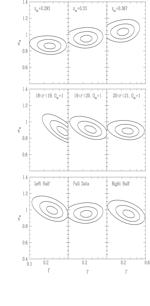
Figure 9: The effects of various systematics on the likelihood contours for $\sigma_{8L}$ and $\Gamma$. Top row: Varying $dn/dz$ to have median redshifts $z_{m}=0.293,0.33,0.367$, respectively. The middle uses the best fit $dn/dz$, bracketed by the lower and upper bounds of the estimated distribution (dashed lines on Figure 1. The magnitude range used is $20<r^{*}<21$. Middle row: Varying the assumed cosmology from our fiducial model to $\Omega_{m}=1,\Omega_{\Lambda}=0.0$. The three magnitude bins are as in figure 7. Bottom row: Varying the angular extent of the stripe. We split our data along the RA direction into two halves, each 2.5^∘x44^∘. The left and right panels show $190^{\circ}\leq\alpha\leq 234^{\circ}$ and $146^{\circ}\leq\alpha\leq 190^{\circ}$, respectively. The middle panel shows the full stripe as in figure 7. The tilting of the likelihood contours in the half-data stripes shows that reduced coverage in angular scale leads to a correlation between $\Gamma$ and $\sigma_{8L}$. The magnitude range is $20<r^{*}<21$. Agreement between the two halves, which have very different average seeing, indicates that seeing does not affect these results.

Figure 9 shows that this scaling relation works remarkably well. In this test we compute likelihood contours for $\sigma_{8L}$ and $\Gamma$ as before, but vary the median redshift of the assumed redshift distribution for the $20<r^{*}<21$ sample. The comoving distances of the galaxies can also be changed by varying the cosmological parameters $\Omega_{m}$ and $\Omega_{\Lambda}$, which alters the redshift-distance relation and the evolution of galaxy clustering. To test the effect of cosmology, in figure 9 we show likelihood contours of $\sigma_{8L}$ and $\Gamma$ for the $20<r^{*}<21$ sample, this time using $\Omega_{m}=1,\Omega_{\Lambda}=0$. This may be compared with figure 7 for the $\Omega_{m}=0.3,\Omega_{\Lambda}=0.7$ model. Again, the predicted scaling of $\sigma_{8L}$ and $\Gamma$ is consistent with the differences in the parameters obtained for the two models. We find that the scaling of $\sigma_{8L}$ and $\Gamma$ in our $20<r^{*}<21$ sample, is well fit by

$$\Gamma\sigma_{8L}=0.173\pm 0.002$$ (19)

in these tests where we vary the redshift distribution or the cosmological model.

Finally, the evolution of galaxy clustering may differ from the evolution of matter clustering; in our models we assume that they evolve identically. Extant constraints on the amplitude of mass clustering suggest $\sigma_{8L}({\rm mass})\approx 1$ and we find $\sigma_{8L}({\rm galaxies})\approx 1$ in these samples, so the average bias between these galaxies and the underlying mass distribution is relatively small. Thus, our assumption is roughly correct for modes in the linear regime, which dominate our results. However, the observed galaxy clustering amplitude is an average over a heterogeneous population, whose constituents may undergo different clustering evolution. Thus, in detail, there may be mild shifts between the results derived from the different magnitude cuts, which sample somewhat different populations, not to mention possible color/morphological type effects.

4.3 Subsamples of the data set: effects of seeing and angular coverage

The effects of seeing and galactic extinction are extensively discussed by Scranton et al. (2001). With the Bayesian star-galaxy separation method, these effects are shown to be negligible for the analysis of galaxy clustering up to the magnitude limit used in this paper. Here we perform a further test for the possible effects of variable seeing by subdividing the data into two halves, one of which suffered from substantially poorer seeing. As shown in figure 9, we verify that the power spectrum parameters we obtain are fully consistent between the two halves, each with different median seeing, and the full data set. Note that reducing the area of sky increases the covariance between $\sigma_{8L}$ and $\Gamma$ because the fits increasingly depend on wavelength modes that lie to one side of the peak of the power spectrum, as discussed in section 4.1.

5 Discussion

Using only the first 1/50 of the SDSS imaging survey we obtain strong constraints on the shape and amplitude of the three-dimensional power spectrum. Despite lacking redshifts, this photometric sample covering 222 sq. degrees yields uncertainties on $\Gamma$ that are only slightly larger than those estimated from the 2dFGRS sample of 160,000 spectroscopic redshifts (Percival et al. 2001), the largest redshift survey to date. For the faintest apparent magnitude subsample that we examine, $20<r^{*}<21$, the fitted parameters of the power spectrum extrapolated to $z=0$ are $\Gamma=0.188\pm 0.04$ and $\sigma_{8L}=0.915\pm 0.06$ ($1\sigma$ uncertainties from marginalizing over one parameter at a time). We find a trend toward larger $\Gamma$ in our brightest subsample, which reaches into mildly nonlinear scales, biasing the $\Gamma$ estimate. Thus, the $20<r^{*}<21$ sample yields the best estimate of the linear power spectrum because it probes the largest angular scales and is not affected by nonlinearity.

The ability to quickly identify modes that are useful for linear power spectrum estimation is a strong advantage of the KL analysis method. For our stripe-like sky geometry, the eigenmodes naturally segregate into modes that probe large wavelengths along the stripe, short wavelengths across the stripe, and mixtures of the two. Examination of the range of Fourier modes probed by the KL eigenmodes of the sample shows that the highest signal-to-noise KL modes are sensitive primarily to large wavelength fluctuations that lie along the right ascension axis of the stripe. We find that these modes probe scales beyond the peak of the best-fit CDM-like power spectrum. In other words, the KL modes make optimal use of the widest direction of our sample area. For the deepest sample we examine, $20<r^{*}<21$ which has $z_{m}=0.33$, the peak sensitivities of the ten highest signal-to-noise modes are all at comoving wavelength $2\pi/k>200h^{-1}$Mpc. We examine the sensitivity of the fitted parameters to the number of modes used in the analysis, plot the wavenumbers probed by these modes and, as we expect, find that the fitting is stable when nonlinear modes are excluded.

Various estimates of the power spectrum from the SDSS EDR-P sample are also provided by Connolly et al. (2001), Dodelson et al. (2001), Tegmark et al. (2001), and from a galaxy redshift sample over a similar region of the SDSS by Zehavi et al. (2001). In all of the analyses of the SDSS EDR-P photometric sample, we find that the fitted parameters depend on how we choose to limit the range of wavelength scales used in the fitting procedure. Inclusion of nonlinear modes tends to raise $\Gamma$ and lower $\sigma_{8L}$ (see section 4.1). Thus, small variations among the fitted parameters arise when using different estimation methods because they use different projections of the data (KL eigenmodes, spherical harmonics, angular pair counts), which vary in the manner in which they segregate power at linear vs. nonlinear scales. The ease with which one can examine the same range of scales depends on the method.

For this first assay of the KL method on a photometric sample, we choose to limit the estimated parameters to the shape, represented by $\Gamma$ and extrapolated linear amplitude $\sigma_{8L}$. Larger galaxy samples and CMB data can probe the matter density parameter $\Omega_{m}h^{2}$ and baryon to total matter ratio $\Omega_{b}/\Omega_{m}$ separately rather than $\Gamma$. Percival et al. (2001) argue that the 2dFGRS is large enough to do so. They obtain $\Omega_{m}h=0.20\pm 0.03$ and $\Omega_{b}/\Omega_{m}=0.15\pm 0.07$ for a redshift sample of 160,000 galaxies to $b_{J}=19.45$. We can use the approximate formula of Sugiyama (1995) to convert this to the shape parameter, $\Gamma=\Omega_{m}h/\exp(\Omega_{b}(1+\sqrt{2h}/\Omega_{m}))$. For the estimates of Percival et al., this yields $\Gamma=0.17\pm 0.03$, with which we agree within 1$\sigma$ for our best (deepest) sample.

It is also instructive to compare with parameters estimated from recent CMB anisotropy experiments. Results from DASI and Boomerang (Pryke et al. 2001, Netterfield et al. 2001) correspond to

$$0.16<\Omega_{m}h<0.27;\qquad 0.10<\Omega_{b}/\Omega_{m}<0.18.$$ (20)

These bounds are based on combining their estimates for the dark matter, baryonic matter and errors with a strong Hubble prior of $h=0.72\pm 0.08$ (HST Key Project – Freedman et al. 2001), and assuming the distributions are disjoint and normally distributed with the quoted errors.

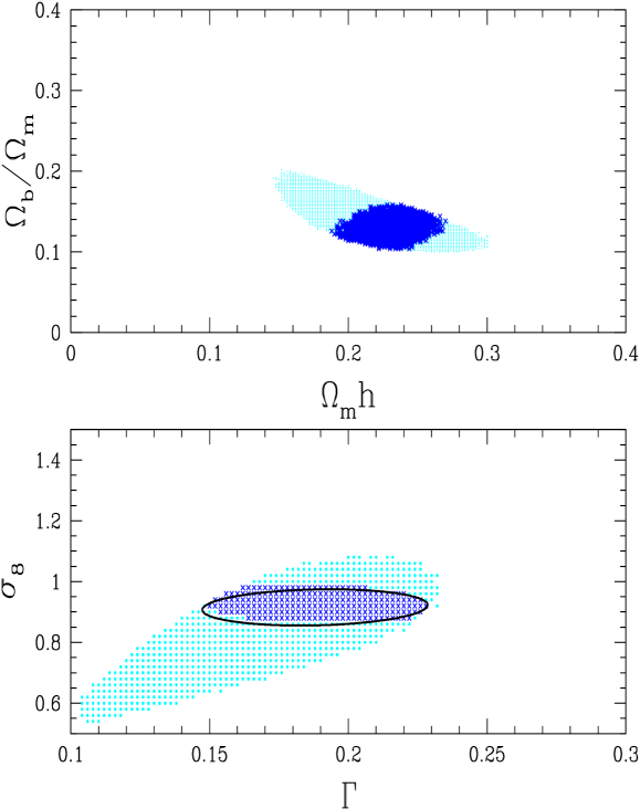
Figure 10: A plot of the CMB constraints on $\Omega_{b}/\Omega_{m}$ vs $\Omega_{m}h$, and $\Gamma$ vs $\sigma_{8L}$. The points were generated by $10^{6}$ Monte Carlo simulations, assuming gaussian distributions for $\Omega_{c}h^{2}$, $\Omega_{b}h^{2}$, and $n$ from DASI (Pryke et al 2001) and BOOMERANG (Netterfield et al 2001), as well as $h=0.72\pm 0.08$. The upper plot shows the 68% confidence region in the $\Omega_{b}/\Omega_{m}$ vs $\Omega_{m}h$ plane, and the bottom plot shows the 68% confidence region in the $\sigma_{8L}$ vs $\Gamma$ plane. Our fiducial contour is marked as the ellipse on the lower plot. The plots use dark x’s to mark those cells for which at least 25% of the models fall in the $\Gamma-\sigma_{8L}$ error ellipse of our paper. These dark x’s may thus be regarded as the set of model parameters jointly allowed by the CMB and our LSS constraints. Values as high as $\Gamma=0.24$ and as low as $\Gamma=0.15$ are possible. The points on the upper plot form a smooth band; the CMB and LSS constraints are almost orthogonal.

A plot of the CMB constraints on $\Omega_{b}/\Omega_{m}$ vs $\Omega_{m}h$, and $\Gamma$ vs $\sigma_{8L}$ is shown in Figure 10. The points were generated by $10^{6}$ Monte Carlo simulations, assuming Gaussian distributions for $\Omega_{c}h^{2}$, $\Omega_{b}h^{2}$, and $n$ from DASI (Pryke et al 2001) and BOOMERANG (Netterfield et al 2001), as well as $h=0.72\pm 0.08$. The upper plot shows the 68% confidence region in the $\Omega_{b}/\Omega_{M}$ vs $\Omega_{M}h$ plane, and the bottom plot shows the 68% confidence region in the $\sigma_{8L}$ vs $\Gamma$ plane. Our fiducial contour is marked as the ellipse on the lower plot. The plots use dark x’s to mark those cells for which at least 25% of the models fall in the $\Gamma-\sigma_{8L}$ error ellipse of our paper. These dark x’s may thus be regarded as the set of model parameters jointly allowed by the CMB and our LSS constraints. Values as high as $\Gamma=0.24$ and as low as $\Gamma=0.15$ are possible. The points on the upper plot form a smooth band; the CMB and LSS constraints are almost orthogonal. The values for $\Omega_{b}/\Omega_{M}$ are in excellent agreement with the most recent results from Big Bang Nucleosynthesis (Burles et al 2001).

We also examine the evolution of clustering by estimating parameters of the galaxy power spectrum at the effective redshift of each subsample (rather than extrapolating that clustering to zero redshift as in the previous analyses). Note that different ranges of absolute magnitude are sampled by the different apparent magnitude slices, thus luminosity dependence of clustering complicates interpretation of these results; the signal of genuine clustering evolution remains to be disentangled from the systematic effect of varying the intrinsic luminosity of galaxies in the three apparent-magnitude limited subsamples that we examine.

This analysis has only used about 2% of the whole SDSS data set. It is clear that the statistical accuracy is going to improve dramatically for the whole data set. Systematic uncertainties, like photometric calibrations and extinction corrections will be the limiting factor at that point, though these are also going to improve by factors of several. Photometric redshifts (Connolly et al 1995) offer an elegant extension of this method: by selecting several thick photo-z slices we can measure the shape parameters of the power spectrum at several redshifts, thus measuring evolution in the clustering. By deriving an SED type for each galaxy we can also create rest-frame selected samples at different redshifts. This paper has shown that even without redshifts, but with accurate photometry one can derive surprisingly accurate information about the shape of the primordial fluctuations.

Figure 1: Redshift distributions assumed for the magnitude bins $18<r^{*}<19$, $19<r^{*}<20$ and $20<r^{*}<21$ shown by solid lines corresponding to increasing values of the median redshift. The two dashed curves show the uncertainty in the estimated redshift distribution for the $20<r^{*}<21$ bin.

Figure 2: The eigenvalues of the correlation matrix are plotted vs. the mode number of the KL eigenmodes for the magnitude bin $20<r^{*}<21$ (upper panel). These are ordered by decreasing signal-to-noise, but the normalization is arbitrary. The transition in slope at around mode 40 approximately corresponds to the aspect ratio of our $5\times 175$ pixel map, thus marking the transition from purely “longitudinal” or 1-dimensional to genuine 2-dimensional modes. The lower panel shows the effective wavenumber for a given mode, corresponding to the peak of the power spectrum of the mode, where the angular wavelength was converted to transverse length at the mode of our redshift distribution, using our fiducial cosmology.

Figure 3: Selected KL modes (mode numbers, or ranks 1,2,4,16 and 300) are shown for the $2.5^{\circ}\times 90^{\circ}$ geometry of the data stripe. The lowest panel shows mode 300, showing the smallest length scales, corresponding to about 0.5^∘, used in the parameter estimation.

Figure 4: The input and reconstructed pixellized density field of the data. The upper panel shows the data binned in pixels 0.5^∘ on a side. The middle panel shows the reconstructed density using the first 300 KL modes. The bottom panel shows the residuals.

Figure 5: The peak wavenumber corresponding to the first 300 KL modes for the $20<r^{*}<21$ magnitude bin. The modes are numbered by their eigenvalues (Figure 2). The modes 1-100 are shown as black dots, the modes 101-200 are stars, the modes 201-250 are x’s and 251-300 are open circles. For some of the modes we also show the contours of the power spectrum corresponding to the given mode. The elongation of the modes in $k$-space is due to the extreme aspect ratio of our geometry. The peak of the power spectrum is at about $k=0.02h/{\rm Mpc}$, within which there are six modes with high signal-to-noise.

Figure 6: Histogram of the first 300 KL coefficients for the $20<r^{*}<21$ sample, normalized as $b_{n}=B_{n}/\sqrt{\lambda_{n}}$. These should have a normal Gaussian distribution (shown by the solid curve) for a Gaussian density field. The agreement of the measured histogram with the Gaussian curve demonstrates that the number of KL modes has been chosen appropriately – there are no features arising from small-scale nonlinearity/non-Gaussianity.

Figure 7: Likelihood contours (plotted at 1, 2, and $3\sigma$) for $\sigma_{8L}$ and the shape parameter $\Gamma$ for three magnitude bins as indicated in the panels. These assume an $\Omega_{m}=0.3,\Omega_{\Lambda}=0.7$ cosmology. The redshift distribution dn/dz$\ \propto z^{2}e^{-(z/z_{0})^{1.5}}\$ with median redshifts $z_{m}=0.17,0.24,0.33$ is used for the three panels respectively ($z_{m}=1.412z_{0}$). The KL expansion was truncated at 300 modes in the upper three panels. To ensure that only the linear modes are used, in the lower panels the expansion was truncated at 60, 150 and 250 modes (from left to right). The panel in the lower right is our best fit.

Figure 8: Likelihood contours for $\sigma_{8L}$ and $\Gamma$ for various truncations of the KL basis, using the magnitude bin $20<r^{*}<21$. As the number of modes is cut, we see that the likelihood contours become broader, as the information used in the fitting process is reduced, and a positive correlation between $\sigma_{8L}$ and $\Gamma$ appears, since the low order modes mostly probe the rising slope of $P(k)$. The central values of $\sigma_{8L}$ and $\Gamma$ are nearly identical for 200 or 250 modes (middle panel) but these parameters are larger for 300 modes, with no significant increase in precision. These extra 50 modes start to probe power in the mildly nonlinear regime (see figure 5), yielding a shift in the estimated parameters in the expected sense. The figure shows that truncating at 250 modes provides small error bars and avoids leakage from nonlinear scales at the same time.

References

- (1) Baugh, C. M., Efstathiou, G., 1994, MNRAS, 267, 323
- (2) Burles, S., Nollett, K.M., & Turner, M.S. 2001, ApJL, in press, astro-ph/0010171
- (3) Cole, S., Hatton, S., Weinberg, D.H., Frenk, C.S. 1998, MNRAS, 300, 945
- (4) Connolly, A. J., Csabai, I., Szalay, A. S., Koo, D. C., Kron, R. C., & Munn, J. A., 1995, AJ, 110, 2655
- (5) Connolly, A. J. et al 2001, submitted to ApJ
- (6) Dodelson, S. et al 2001, submitted to ApJ
- (7) Dodelson, S., Gaztanaga, E., 2000, MNRAS, 312, 774
- (8) Efstathiou, G., Bond, J.R., White, S.D.M. 1992, MNRAS, 258, 1P
- (9) Eisenstein, D. J., Zaldarriaga, M., 2001, ApJ, 546, 7
- (10) Efstathiou, G., Moody, S. J., 2001, astro-ph/0010478
- (11) Freedman, W.L. et al. 2001, submitted to ApJ, astro-ph/0012376
- (12) Fukugita, M. et al 1996, AJ 111, 1748
- (13) Gunn, J.E.G., Carr, M.A., Rockosi, C. Segiguchi, M. et al 1998, AJ, 116, 3040
- (14) Halverson, N.W. et al. 2001, submitted to ApJ, astro-ph/0104489
- (15) Hamilton, A. J. S., Tegmark, M., Padmanabhan, N., 2000, MNRAS, 317, L23
- (16) Karhunen, H. 1947, Ann. Acad. Science Finn. Ser. A.I. 37
- (17) Limber, D. N., 1953, ApJ, 117, 134
- (18) Lin, H., Yee, H.K.C., Carlberg, R.G., Morris, S.L., Sawicki, M., Patton, D.R., Wirth, G., Shepherd, C.W. 1999, 518, 533
- (19) Lee, A.T. et al. 2001, submitted to ApJ, astro-ph/0104459
- (20) Loève, M. 1948, Processes Stochastiques et Mouvement Brownien, (Hermann, Paris France)
- (21) Lupton R. H. et al 2001, in ASP Conf. Ser. 238, Astronomical Data Analysis Software and Systems X, ed. F. R. Harnden, Jr., F. A. Primini, and H. E. Payne (San Francisco: Astr. Spc. Pac.), in press (astro-ph/0101420)
- (22) Matsubara, T., Szalay, A. S., Landy, S. D., 2000, ApJ, 535, L1
- (23) Netterfield, C.B. et al. 2001, submitted to ApJ, astro-ph/0104460
- (24) Peacock, J.A., Dodds, S.J. 1994, MNRAS, 267, 1020
- (25) Peebles, P. J. E. 1980, The Large-Scale Structure of the Universe (Princeton: Princeton University Press)
- (26) Percival, W.J., et al. 2001, submitted to MNRAS, astro-ph/0105252
- (27) Pryke, C., Halvorsen, N.W., Leitch, E.M., Kovac, J., Carlstrom, J.E., Holzapfel, W.L., & Dragovan, M. 2001, submitted to ApJ, astro-ph/0104490
- (28) Scranton, R. et al 2001, submitted to ApJ
- (29) Stoughton, C. et al 2001, submitted to AJ
- (30) Sugiyama, N. 1995, ApJS, 100, 281
- (31) Tegmark, M. et al 2001, submitted to ApJ
- (32) Vogeley, M.S., Szalay, A.S., 1996, ApJ, 465, 34
- (33) York, D.G. et al 2000, AJ, 120, 1579
- (34) Zehavi, I. et al 2001, submitted to ApJ