Analysis of Systematic Effects and Statistical Uncertainties in Angular Clustering of Galaxies from Early SDSS Data

Abstract

The angular distribution of galaxies encodes a wealth of information about large scale structure. Ultimately, the Sloan Digital Sky Survey (SDSS) will record the angular positions of order $10^{8}$ galaxies in five bands, adding significantly to the cosmological constraints. This is the first in a series of papers analyzing a rectangular stripe $2.5^{\circ}\times 90^{\circ}$ from early SDSS data. We present the angular correlation function for galaxies in four separate magnitude bins on angular scales ranging from $0.003$ degrees to $15$ degrees. Much of the focus of this paper is on potential systematic effects. We show that the final galaxy catalog – with the mask accounting for regions of poor seeing, reddening, bright stars, etc. – is free from external and internal systematic effects for galaxies brighter than $r^{*}=22$. Our estimator of the angular correlation function includes the effects of the integral constraint and the mask. The full covariance matrix of errors in these estimates is derived using mock catalogs with further estimates using a number of other methods.

1 Introduction

One of the most direct and powerful probes of models of structure formation is the two-point function for galaxies, either the correlation function in real space or the power spectrum in Fourier space. At least on large scales, observations of the power spectrum can be directly compared with predictions of theoretical models. Indeed, this comparison is one of the strongest arguments (see e.g. Peacock & Dodds, 1994) to date against the simplest Cold Dark Matter model with a matter density equal to the critical density.

There are several ways to measure the power spectrum. The most direct is to use a redshift survey, which contains information not only about the two dimensional angular position of each galaxy but also about its radial distance from us. Angular surveys do not have any radial information, but they are often just as powerful probes of the power spectrum because they contain many more galaxies than do redshift surveys. Examples of angular surveys which have been used to measure the power spectrum are the APM (Maddox et al., 1990; Efstathiou & Moody, 2000) and the Edinburgh/Durham Southern Galaxy Catalogue (Collins, Nichol & Lumsden, 1992; Huterer, Knox & Nichol, 2000).

The Sloan Digital Sky Survey (SDSS; York et al. 2000; Gunn et al. 1998; Fukugita et al. 1996) will ultimately obtain angular positions for $\sim 10^{8}$ galaxies and redshifts for $10^{6}$ galaxies. Both will be powerful probes of cosmological models. This paper analyzes the angular correlation function from early, imaging data taken during the photometric commissioning of SDSS. The survey data will be of higher quality (mainly due to better image quality and photometric calibration), so some of the systematic effects analyzed here will be less severe in the full survey. Likewise, since the data is collected digitally, we expect to be free of a number of systematic effects related to earlier surveys using scanned photographic plates (Nichol & Collins, 1993; Maddox et al. 1996).

The data were taken in two nights in March, 1999 with the SDSS Camera (Gunn et al. 1998) on the 2.5m telescope (SDSS Runs 752/756). The area surveyed is centered on the Celestial Equator $2.52$ degrees wide by approximately $90$ degrees long. In equatorial coordinates, the observed region runs from $9^{h}40^{m}48^{s}$ to $15^{h}45^{m}12^{s}$ in $\alpha$ (J2000), putting the very ends of the run at somewhat low Galactic latitudes. This area was imaged in two interlaced strips of six columns (or “scanlines”) which together form a continuous region. Although each object is sampled in five bands ($u^{\prime},g^{\prime},r^{\prime},i^{\prime},z^{\prime}$; Fukugita et al. 1996), the objects chosen here were selected based on their $r^{*}$ model magnitudes (where $r^{*}$ refers to the photometric calibration used in the Early Data Release (EDR; Stoughton, et al. (2001)) for the standard band-pass filter $r^{\prime}$). Ultimately, photometric redshifts can be obtained by using the multi-band information, but here we make no estimate of the radial distance of each object. This pair of runs has been used in previous early SDSS papers analyzing the galaxy luminosity function (Blanton et al. 2001), number counts (Yasuda et al. 2001) and colors (Shimasaku et al. 2001; Strateva et al. 2001).

Photometric calibration is carried out using an auxiliary 20” telescope adjacent to the SDSS 2.5m telescope (the ‘Photometric Telescope’, or PT). The PT observes a set of standard stars which have been calibrated to the SDSS filter system (Smith et al. 2001) in order to determine the atmospheric extinction of a given night. Additionally, the PT observes regions of the sky (‘secondary standards’) which overlap the imaging scans, setting the photometric zeropoints for these. For runs 752 and 756, 11 and 16 secondary patches were observed, respectively. In later calibrations, the photometric zeropoint of each chip was assumed to be constant through each run, but the calibration of the data we used allowed for the zeropoint to vary from patch to patch. The zeropoints from each secondary patch typically agreed with each other to 0.013 magnitudes in $r^{*}$.

Every object in the survey is assigned a probability that it is a galaxy based upon its morphology. The basic algorithm used to assign these probabilities is discussed in §2. In §3, we test the star/galaxy separation scheme with a wide variety of systematic checks. We show there that the separation predictably does not work well in regions of very poor seeing, so we mask out the poor seeing regions. The resultant mask is presented in §4; it accounts for seeing, reddening, bright stars, and saturated CCD columns. In §5, we look for systematic effects due to uncertainties in magnitudes. Varying responses in different parts of the camera are another possible source of systematic errors, both within a given scanline and from scanline to scanline. We check for these in §6.

The final third of the paper discusses technical details related specifically to the measurement of the angular correlation ($w(\theta)$). Two estimators are used to estimate $w(\theta)$, one a point-based approach, the other cell-based. While they are equivalent on scales larger than a cell size, each carries with computational advantages and disadvantages. These are discussed in §7, as is the integral constraint which becomes important on large scales (here on the order of a degree). The errors on $w(\theta)$ are particularly important because (i) they are due to both Poisson statistics and cosmic variance and (ii) they are highly correlated from bin to bin. We present estimates of the full covariance matrix in §8 using four techniques, each with its regime of validity. Finally, we offer some conclusions in §9.

With this prescription for avoiding photometric systematic effects in hand, there are a number of clustering measurements possible. A companion paper (Connolly et al. 2001) will present the final measurement of $w(\theta)$ along with comparisons to previously published measurements. Additionally, Tegmark et al. (2001) gives a measurement of the angular power spectrum ($C_{l}$). Dodelson et al. (2001) inverts the angular correlations and angular power spectra to extract the three-dimensional power spectrum, which will then be used to do parameter estimation. In parallel, Szalay et al. (2001) performs a Karhunen-Loéve decomposition of the data, allowing for a direct estimation of the $\Gamma$ and $\sigma_{8}$ parameters. Finally, Szapudi et al. (2001) presents the higher order correlation functions for the data. All of these companion papers use a common data set, the EDR-P, taken from the Early Data Release and extended to include the galaxy Probabilities described below.

2 Star/Galaxy Separation

The photometric data are processed using a series of interlocking pipelines that flat-field the images, match up the data in the different bands, measure the properties of all detected objects, and apply astrometric and photometric calibrations. A large number of attributes are measured for each object, including a variety of aperture and model magnitudes.

Our object classification algorithm uses the outputs of this pipeline to separate stars and galaxies independent of the standard pipeline’s binary decision about the stellar or galactic nature of a given object. The pipeline’s separation works well at relatively bright magnitudes where the distinction between galaxies and stars is clear-cut, but at the faint end of the magnitude range there is a definite need to know the degree of certainty in calling an object a star or a galaxy. With that in mind, we developed a Bayesian method of star/galaxy separation based upon the outputs of the pipeline. This method has proven effective enough that it will be a standard output of the future versions of the pipeline. The details of this separation method are given in Lupton et al. (2001) along with more detailed descriptions of the processing pipeline and tests of the reliability of the morphological parameters. For pedagogical purposes, we present an outline of the method employed for star/galaxy separation below.

2.1 Separation Method

The data processing pipeline provides a number of standard outputs which could be used for star/galaxy separation. For our purposes, four magnitude measures are of principal interest: PSF magnitudes, exponential magnitudes, deVaucouleurs magnitudes and model magnitudes. The first of these is simply the magnitude of a given object fit to the point-spread function (PSF) calculated locally based upon the measured PSF of nearby bright stars. The exponential and deVaucouleurs magnitudes are measured within two dimensional profiles where the axis ratio and scale lengths are fit to the object; in addition the model has been convolved with the PSF. Model magnitudes are the best fit of either the exponential or deVaucouleurs model in the $r^{*}$ band.

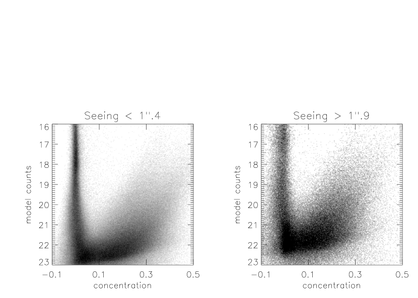
Figure 1: Concentration-magnitude diagrams for regions of good (left) and bad (right) seeing. Areas of poor seeing show increased width of the stellar locus, brighter merging of the stellar and galactic loci and a shifting of the faint galactic locus centroid toward that of the stellar locus.

From these magnitudes, we derive our central tool for star/galaxy separation, the concentration, which is defined for each object as $c\equiv r^{*}_{\rm PSF}-r^{*}_{\rm EXP}$, where $r^{*}_{\rm PSF}$ is the $r^{*}$ PSF magnitude and $r^{*}_{\rm EXP}$ is the exponential magnitude. In the case of a star, the concentration parameter should be very close to zero. For a galaxy, however, the concentration is positive for bright magnitudes and then tends toward zero at fainter magnitudes as the galaxies become less and less resolved. Figure 1 shows the behavior of this parameter for several thousand objects over a range of model magnitudes in the $r^{*}$ band.

The most striking feature of this plot is the clear separation between the stellar and galactic loci at bright magnitudes. For fainter magnitudes, this clean separation degrades as galaxies become less resolved and magnitude errors increase. Clearly, this will lead to some cross-contamination between the two populations, which we will quantify below.

2.2 Bayesian Probabilities

While a straight-line binary cut in concentration-magnitude space (as given by the object type classification in the standard pipeline) has the advantage of simplicity (provided that one can adjust the location and orientation of the demarcation line to maximize the selection efficiency), it produces little measure of the statistical confidence in the classification of each object. The following gives a brief description of the probabilistic method of separation used in our analysis of $w(\theta)$. Again, this method will be covered in greater detail in Lupton, et al. (2001).

Using the standard Bayesian formalism, we can express the probability that a given object is a galaxy (G) in terms of its magnitude ($m$) and concentration parameter ($c$) as

$$P(G|m,c)=\frac{P(m,c|G)P(G)}{P(m,c)},$$ (1)

where $P(m,c|G)$ is the posterior probability, $P(G)$ is the prior and $P(m,c)$ is the global likelihood. We can pull magnitude out of the expression for the posterior probability as

$$P(G|m,c)=\frac{P(c|m,G)P(m|G)P(G)}{P(m,c)},$$ (2)

where $P(m|G)$ is simply the galaxy number count relation for a given magnitude. We can find this by using a simple straight line cut for the brighter magnitude objects (approximately $17\leq r^{*}\leq 19$) where the stellar and galactic populations are well separated. We can fit an exponential curve to this relation and normalize it over the magnitude range to find the probability for a given magnitude. Yasuda et al. (2001) have measured this relation from the same SDSS data; our independent measurement confirms their result for the fainter end of their sample.

Using the fact that the stellar and galactic probabilities for a given object must sum to one, we can re-write the above as

$$P(G|m,c)=\left(1+\frac{P(c|m,S)P(m|S)P(S)}{P(c|m,G)P(m|G)P(G)}\right)^{-1},$$ (3)

Again, we can use the empirical results from the easily separable bright objects to find $P(m|G)$ and $P(m|S)$, taking into account the variation in stellar density as a function of Galactic coordinates. In practice, the sensitivity of the separation to the star-galaxy ratio is generally quite low for realistic values. More explicitly, since we will be calculating these quantities over a small, finite magnitude range, we can re-express the above as

$$P(G|m,c)=\left(1+\frac{P(c|m,S)P(S|m)}{P(c|m,G)P(G|m)}\right)^{-1},$$ (4)

where $P(S|m)$ and $P(G|m)$ folds in the relative abundance of galaxies and stars due to changes in Galactic latitude. This leaves us only $P(c|m,S)$ and $P(c|m,G)$ to calculate. To find these probabilities, we bin the data from the magnitude-concentration plot in magnitude, resulting in histograms like that in Figure 2. After applying a simple transformation on the concentration to rein in the tail on the galaxy distribution, we fit a Gaussian to the galaxy locus and two Gaussians to the stellar locus (to account for the slightly wider non-Gaussian tails) for all of the magnitude bins. This allows us to interpolate the parameters of the two probability distributions, giving us the galactic and stellar probabilities for a given magnitude and concentration.

With minimal effort, we can expand the above to include information on the seeing conditions ($s$) for a given object, resulting in

$$P(G|m,c,s)=\left(1+\frac{P(c|s,m,S)P(S|m,s)}{P(c|s,m,G)P(G|m,s)}\right)^{-1}.$$ (5)

This extension is needed to compensate for the different behavior of the stellar and galactic loci under different seeing conditions as seen in Figure 1. In regions where the seeing is very good, there is clear separation between the stellar and galactic loci to fainter magnitudes than in those regions with poor seeing. Likewise, the centroid of the galactic locus is considerably closer to that of the much wider stellar locus at fainter magnitudes in the bad seeing regions, where the PSF has increased.

In modifying Equation 4 to include seeing in this way, we are assuming that the measurement of the magnitude is unaffected by seeing. For brighter objects this should be true and in the faint limit the effects of the seeing on the magnitude would act in much the same manner for both galaxies and stars since both types of object have nearly the same light distribution. This effect should therefore roughly cancel in Equation 5. This conjecture has been verified by Ivezic et al. (2001) in their examination of objects doubly imaged in those regions where scanlines in interlaced strips overlap (see York et al. (2000) for an explanation of the scanning procedures). They have found that, for reasonably bright objects imaged in very different seeing conditions, the magnitudes are very consistent. Just as importantly, the effect of different seeing on the magnitude was the same for stars and galaxies at the faint limit. Thus, we can safely bin the objects in both magnitude and seeing before fitting the Gaussians to the concentration distributions and then bilinearly interpolate in those variables to find $P(c|s,m,G)$ for a given concentration, magnitude, and seeing.

For the actual form of $P(G|s,m)$ and $P(S|s,m)$, we can use a similar method to that used for the case without seeing included. The effect of worsening seeing is to brighten the faint magnitude limit. Since most of the objects at that limit have similar sizes anyway, we would again expect that the effects for galaxies and stars in that limit would be the same and thus cancel out in the formula. In fact, we can replace $P(G|m,s)$ with $P(G|m)$ and $P(S|m,s)$ with $P(S|m)$ without losing information,

$$P(G|m,c,s)=\left(1+\frac{P(c|s,m,S)P(S|m)}{P(c|s,m,G)P(G|m)}\right)^{-1}.$$ (6)

With a star/galaxy separation scheme in hand, we must verify that applying the method results in a uniform sample of galaxies across the field of view. This will make checking the variation of the sample against possible sources of contamination paramount if we want to assure ourselves we are measuring the galaxy clustering independent of systematic effects. As we will show in the following sections, the proper cuts on those systematic contaminants allow us to reliably separate stars from galaxies down to a model magnitude of 22 in $r^{*}$. The efficacy of the original binary galaxy/separation separation has been analyzed by Yasuda et al. (2001) down to $r^{*}\sim 21$. Our tests verify that our probabilistic separation matches this performance and allows us to go to fainter magnitudes where the binary method fails. This allows us to make the four unit magnitude cuts that we will use for the rest of our analysis: $18\leq r^{*}\leq 19$, $19\leq r^{*}\leq 20$, $20\leq r^{*}\leq 21$, and $21\leq r^{*}\leq 22$, with approximately 0.16, 0.31, 0.65 and 1.15 million galaxies, respectively. All of the magnitude cuts are based on the model magnitudes, dereddened using the reddening map of Schlegel, Finkbeiner, & Davis (SFD, 1998).

3 External Systematic Error Sources

By restricting the area of our survey, we can reduce the measured systematic errors in $w(\theta)$ due to variations in seeing and dust extinction to below the errors in the measurement due to cosmic variance and Poisson errors. We are also able to separate the stellar and galaxy populations to the extent that their cross-contamination becomes negligible. In this section, we present various diagnostic tests of the data to determine how best to define the survey area. Although these tests concentrate on the angular correlations, the resulting mask is equally valid for any measurement of angular clustering (e.g. angular power spectrum or KL decomposition).

3.1 Galaxy Densities

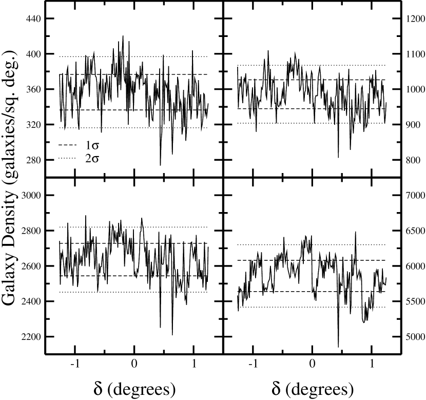
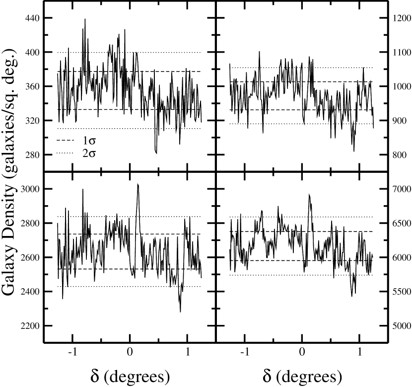
Figure 3: Galaxy density projected along the long axis of the survey area without using a mask (left) and using a mask (right). Clockwise from the upper left, the magnitude bins are $18\leq r^{*}\leq 19$, $19\leq r^{*}\leq 20$, $20\leq r^{*}\leq 21$, $21\leq r^{*}\leq 22$ . Horizontal lines indicate $1\sigma$ and $2\sigma$ limits in the density.

Measuring the galaxy densities projected along the long and short axes of the survey area is the first check that our galaxy sample is reasonably uniform. The first check is verifying that the structure of the scanlines is not reflected in the galaxy densities. The left panel of Figure 3 shows the variation of the galaxy density in the raw data for each of the magnitude bins as a function of declination, with CCD scanlines progressing from left to right; alternating scanlines are observed simultaneously. The width of each scanline is $\sim 0.21^{\circ}$ and the 12 scanlines are split evenly between positive and negative declination.

Here we obtain the galaxy densities by summing the galaxy probabilities of all objects in the region. To first order, the appearance of boundaries between scanlines is minimal, but certainly visible in the break at zero declination, for example. If we apply a mask to the data (the exact details of which are explained and justified in §3.4) to avoid the regions where the data quality is questionable, we get the result plotted in the right panel of Figure 3. The masked sample avoids obvious problems like the sharp dips near $\delta\sim 0.4^{\circ}$ and $0.65^{\circ}$ (explained in §5) and the sharp boundaries between scanlines.

In order to get a more precise idea of what data should be cut out if we want to avoid systematic errors, we need to examine the behavior of the galaxy density while varying some of the possible sources of errors. Once this is done, we will be able to move onto more sophisticate techniques for determining the observational limits on these external sources.

3.2 Seeing Variations

As part of the photometric pipeline, a set of PSF eigencomponents are determined using Karhunen-Loéve decomposition of the bright stars in each field of each scanline (the details of this process are presented in Lupton et al. (2001)). By taking into account the position of these stars, one can use interpolation to reconstruct the PSF from a combination of these eigencomponents for any object in the field. To determine the seeing for each object, we calculated the second moment of each of these eigencomponents and then used the same interpolation scheme to reconstruct the seeing; the seeing is given as 2.355 times the second moment which would give the FWHM under the assumption that the PSF is Gaussian. This allows the seeing to be calculated at any object without the more time consuming process of re-constructing the PSF at that point and calculating its second moment. It should be noted, however, that this definition differs from that used by Yasuda et al. (2001) in their analysis, resulting in qualitative, but not quantitative, agreement between our seeing and theirs.

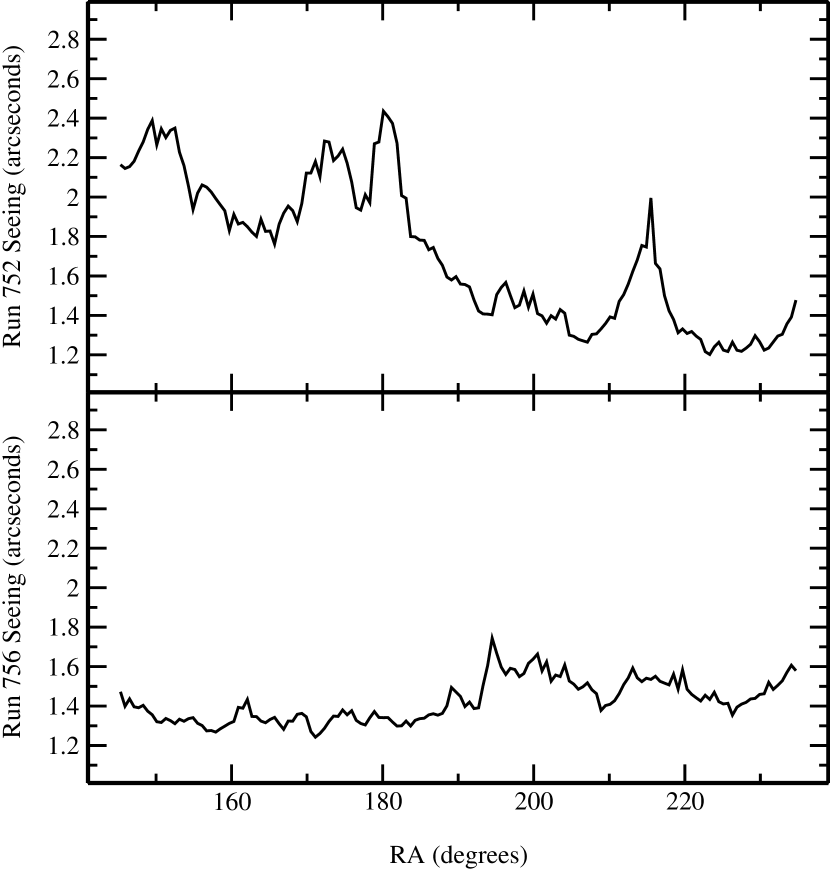
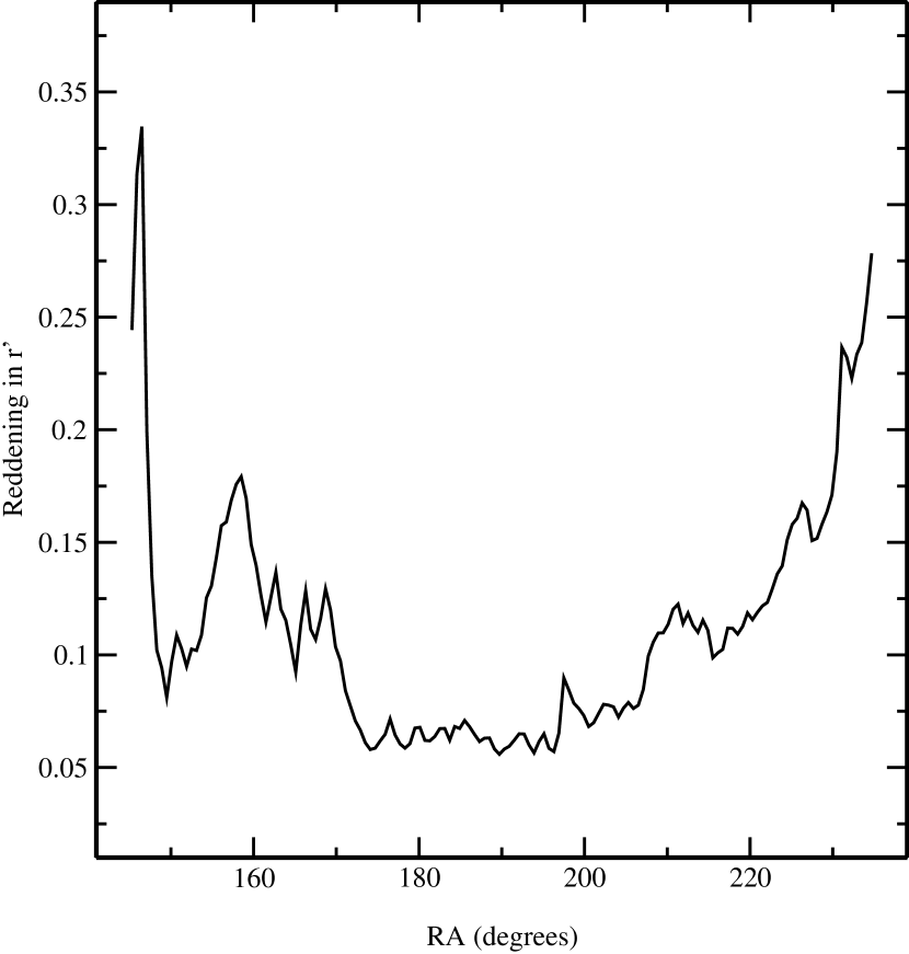
Figure 4: Seeing variations for each of the strips as a function of $\alpha$ (left) and reddening variations as a function of $\alpha$ (right).

The left panel of Figure 4 shows the mean seeing variation across the scanlines for the two runs as a function of right ascension. The seeing for Run 756 is generally well-behaved throughout the course of the run, with only the occasional departure above $1^{\prime\prime}.6$. Run 752, taken two days prior to Run 756, is much more volatile; the entire first half of the run oscillates above $1^{\prime\prime}.8$ and then later the seeing spikes to $2^{\prime\prime}.0$. This structure in the seeing map will require extensive masking and require careful checking against false signal on the scanline scale.

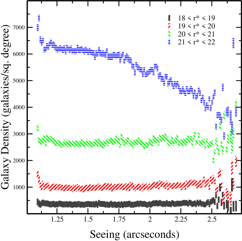
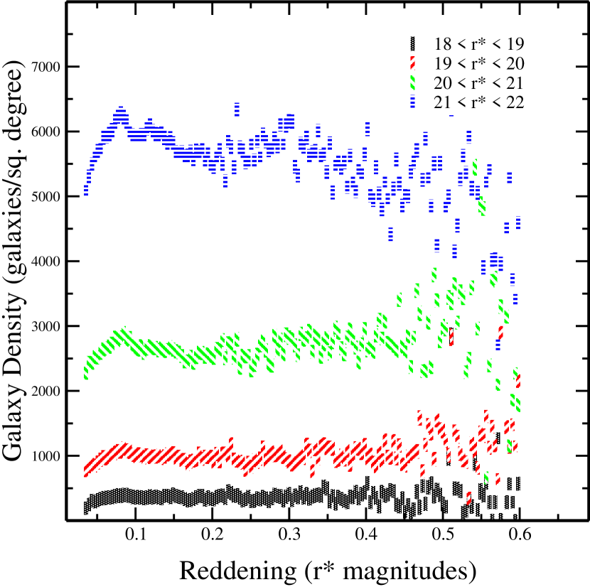
Figure 5: Galaxy density for four magnitude bins as a function of the local seeing (left) and reddening (right).

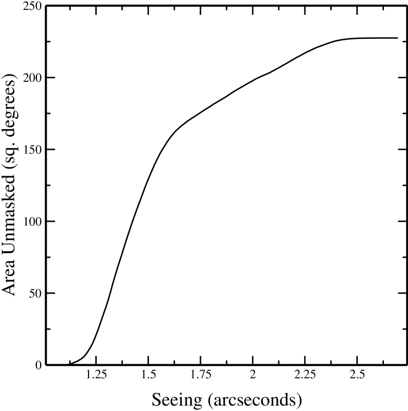
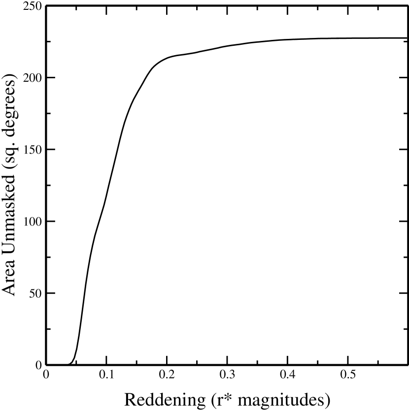
Figure 6: Area left unmasked versus seeing requirement (left) and reddening requirement (right).

In normal survey operations, regions where the seeing degraded to worse than $1^{\prime\prime}.5$ are marked for re-observation, but we did not have that luxury for the commissioning data. In the left panel of Figure 5, we plot the mean galaxy density for the combined stripe as a function of seeing. The galaxy density varies considerably for the faintest magnitude bin over the factor of two in seeing conditions, suggesting that poor seeing lowers the confidence that a given object is a galaxy. Not surprisingly, we also see that the effect of poor seeing is more pronounced at fainter magnitudes than for the brighter objects. Already, the magnitude bin from $21\leq r^{*}\leq 22$ clearly shows that we need to restrict the data to seeing better than $1^{\prime\prime}.75$, but the cross-correlation analysis below will show that the cut needs to be even more restrictive. Figure 6 shows the area which would remain unmasked for a given seeing cut.

3.3 Reddening Variations

Since we are only analyzing the effect of intermediary dust in a single band, the term “reddening” is not as appropriate as “extinction” or “absorption”. However, the magnitude extinction limits that we will set in constructing our mask will refer to the $r^{*}$ element of the reddening output of the photometric pipeline, so we will adopt the use of “reddening” in favor of other alternatives to avoid confusion.

The right panels of Figures 4 and 5 repeat the above analysis in terms of the SFD reddening. The dependence of galaxy density on reddening is weaker than for seeing, but that is to be expected since the survey area does not contain much area where the reddening is significantly higher than $0.2$ magnitudes. Likewise, the small fraction of the area with reddening less than $0.05$ magnitudes makes that density measurement highly dependent on large-scale structure variations in those regions. Still, the fact that the scatter in density is so much larger than the Poisson error for those higher reddening areas suggests that we should consider setting the limit for reddening around $0.2$ magnitudes. Figure 6 shows that the area excluded by such a cut is small.

3.4 Cross-Correlations

Cross-correlations of the galaxy density with maps of external sources offer the most powerful means for checking against contamination in the galaxy sample. Not only can they detect systematic effects, they also offer information on the angular scale of that correlation. This is particularly important in the case of seeing, where we have sharp variations between adjacent scanlines. The caveat with such an approach is the unstated assumption that any variation in the cross-correlations is due to an external source, rather than a variation in the observing system. As we will see in §7, this is a reasonable enough assumption and so we will proceed by cross-correlating the galaxy density with seeing, reddening, stellar density and sky brightness.

To measure the cross-correlations, we generated a pixelized version of the data, breaking the area in each $0.21^{\circ}$ wide scanline into square cells approximately $0.04^{\circ}$ on a side. This gives us five cells in the $\delta$ direction for each scanline and approximately 10,000 for the whole of a given scanline. In each cell, we find the mean seeing, mean reddening in $r^{*}$ and mean sky brightness in $r^{*}$ for all of the objects in the cell, as well as the sum of the galaxy and star likelihoods in each of the four magnitude bins. In principle, these quantities could be found using the seeing, reddening and sky brightness maps independently, but this measure weights our average toward the values most relevant to the objects in the cell.

The size of the cells ensures that the majority of the cells will contain on order 30 objects down to $r^{*}=22$. Smaller cells would allow for greater resolution, but we suspect that most of the systematic effects will occur on the scale size of the scanline or larger. The cell size is also of order the angular resolution of the SFD reddening map. Keeping the mean number of objects per cell high also allows us to ignore cells without any objects (usually due to a missing area in the data, as happens with a single irreducible field in scanline 4 of run 752) without biasing ourselves against genuine voids.

Having the information in this form allows us to calculate the cross-correlation of the galaxy catalog with seeing, reddening, stellar density and sky brightness in each of the magnitude bins for a variety of different seeing and reddening cuts. Once we have established the limits on seeing and reddening necessary to ensure an uncontaminated sample, we then use this pixelization to construct the mask.

To measure the cross-correlation, we first divide the stripe into 35 separate square regions, approximately 2.5 degrees on a side, each containing $\sim 3600$ cells. For each square, we calculate the mean sum of galaxy probabilities ($\bar{n}^{g}$) per cell in a given magnitude bin, as well as the mean for the possible contaminant ($\bar{x}^{c}$), where $x^{c}$ could refer to the sum of the stellar probabilities, mean seeing, etc. This allows us to calculate the fractional galaxy and contaminant overdensity in a given cell $i$,

$$\delta^{g}_{i} = \frac{n^{g}_{i}-\bar{n}^{g}}{\bar{n}^{g}}$$ (7)

$$\delta^{c}_{i} = \frac{x^{c}_{i}-\bar{x}^{c}}{\bar{x}^{c}}$$

The cross-correlation, $w_{gc}(\theta)$, is then simply

$$w_{gc}(\theta_{\alpha})=\frac{\sum_{i,j}\delta^{g}_{i}\delta^{c}_{j}\Theta^{\alpha}_{ij}}{\sum_{i^{*},j^{*}}\Theta^{\alpha}_{i^{*},j^{*}}},$$ (8)

where $\Theta^{\alpha}_{ij}$ is unity if the separation between cells $i$ and $j$ is within angular bin $\theta_{\alpha}$ and zero otherwise. Once the measurement has been done in each of the 35 sub-samples, we calculate the mean ($\bar{w}_{gc}(\theta)$) and error on the mean ($\Delta\bar{w}_{gc}(\theta)$),

$$(\Delta\bar{w}_{gc}(\theta))^{2}=\frac{1}{N^{2}}\sum^{N}_{i=1}(\bar{w}_{gc}(\theta)-w_{gc,i}(\theta))^{2},$$ (9)

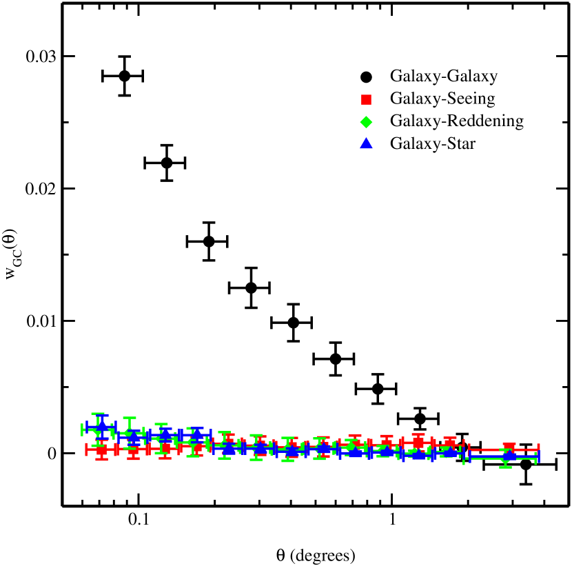
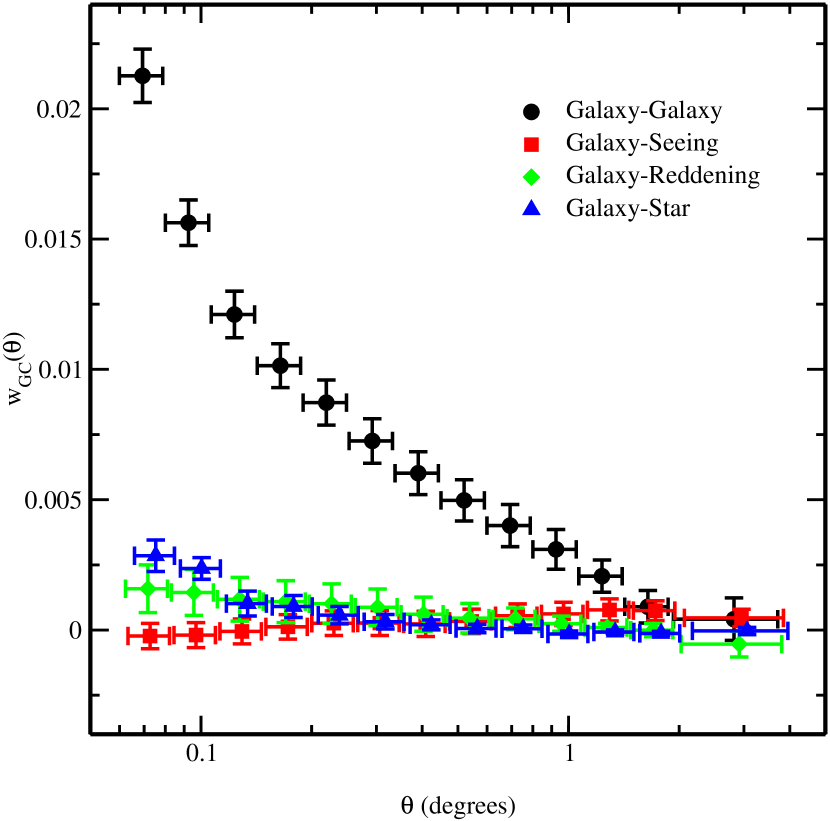
Figure 10: Comparison of the galaxy auto-correlation to the cross-correlation of the galaxy density with seeing, reddening and stellar density, respectively, for the magnitude bins $20\leq r^{*}\leq 21$ (left) and $21\leq r^{*}\leq 22$ (right).

where $N=35$ in this case. In examining the cross-correlations below, one should bear in mind that the galaxy auto-correlation signal we observe at 1 degree is approximately $0.005\pm 0.0025$ for the faintest magnitude bin (see Figure 10). Cross-correlation signals smaller than this value will be over-whelmed by the galaxy signal.

3.4.1 Seeing

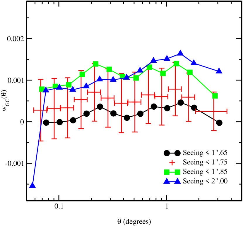
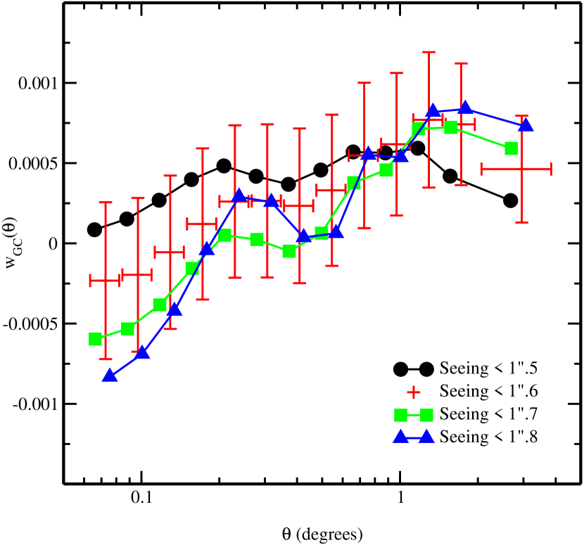
Figure 7: Galaxy-Seeing cross-correlations for magnitude bins $20\leq r^{*}\leq 21$ (left) and $21\leq r^{*}\leq 22$ (right). The size of the error bars on the preferred seeing cut are typical of those for the other seeing cuts, which have been eliminated for clarity.

The cross-correlations between the seeing and the galaxy density for the faintest two magnitude bins in the sample ($20\leq r^{*}\leq 21$ and $21\leq r^{*}\leq 22$) are shown in Figure 7. The goal here should be a flat curve, consistent with zero, and in particular one that shows no structure on the $0.21$ degree scale of the scanlines. Such structure is still seen with a 1”.7 seeing cut for the faintest magnitude bin. The cross-correlation signal is reduced to an acceptable level by using a cut at $1^{\prime\prime}.6$ seeing. It should be noted that even the slight departure from zero seen with this cut is still well below the measurement of $w(\theta)$ on the same angular scales (Figure 10).

Making a cut at $1^{\prime\prime}.6$ is necessary for the faintest bin, but if we are interested in brighter objects, we can relax this cut somewhat. The left panel of Figure 7 shows the same galaxy-seeing cross-correlation for objects with magnitudes $20\leq r^{*}\leq 21$. In this case, we see that we can raise the seeing limit to $1^{\prime\prime}.75$ and still have a cross-correlation consistent with zero, although with some slight variation on the scale of the scanlines. Since we want to include as much area as possible, we use two cuts, one for the faintest bin cutting at seeing of $1^{\prime\prime}.6$ and a second excluding seeing worse than $1.^{\prime\prime}75$ to use for the other three brighter magnitude bins.

3.4.2 Reddening

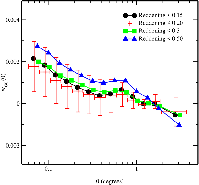
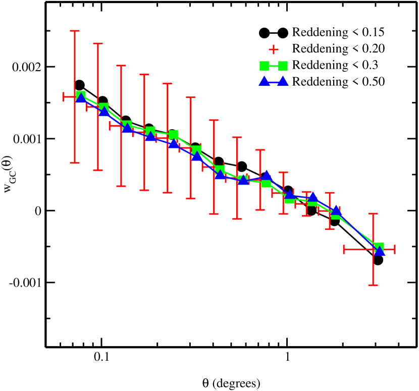
Figure 8: Galaxy-Reddening cross-correlations for magnitude bins $20\leq r^{*}\leq 21$ (left) and $21\leq r^{*}\leq 22$ (right). Again, the error bars on the favored cut are typical of the other limits.

Unlike the galaxy-seeing cross-correlations, there is not a strong relation between tightening the restriction on the allowed reddening in the $r^{*}$ band and improved lack of cross-correlation (Figure 8). This is not terribly surprising given the fluctuations in galaxy density as a function of reddening we saw in Figure 5, particularly for the fainter magnitude bins. However, while the cross-correlations show some degree of angular dependence, they are easily within $2\sigma$ of zero for all angular scales and below the level of the galaxy auto-correlation errors.

Given this, we exclude those regions where the reddening is worse than $0.2$ magnitudes in $r^{*}$ as is suggested by the scatter in galaxy densities at higher reddening levels in Figure 5.

3.4.3 Stellar Density

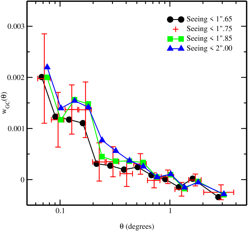
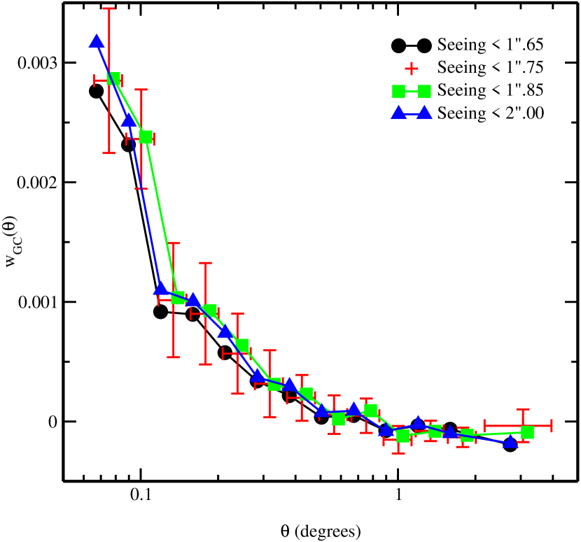
Figure 9: Galaxy-Star cross-correlations for magnitude bins $20\leq r^{*}\leq 21$ (left) and $21\leq r^{*}\leq 22$ (right). The error bars on the favored limit are typical of the other limits.

With perfect star/galaxy separation, we would expect the stellar density auto-correlation to be consistent with zero, except perhaps on the very smallest scales. Thus, in the case where we have mistaken galaxies for stars and vice-versa, we would expect that the cross-correlation of these samples would produce a damped version of the galaxy auto-correlation, diluted by the effectively null stellar auto-correlation. For these tests, we use the limits on the seeing (better than $1^{\prime\prime}.6$ for galaxies fainter than $r^{*}=21$ and better than $1^{\prime\prime}.75$ for brighter galaxies) and reddening (reddening less than 0.2 in $r^{*}$) established in §3.4.1 and §3.4.2. As shown in Figure 9, the cross-correlation between the galactic and stellar populations is within the $2\sigma$ limit of zero for magnitudes brighter than $r^{*}\sim 21$. For the faintest magnitude bin, however, there is a definite correlation between the two populations at small angles, again most likely due to some leakage between the two samples. However, we can see from Figure 10 that the deviation from zero for the star-galaxy cross-correlation is not only much less than the galaxy-galaxy auto-correlation itself , but is also less than the error on that measurement even for the faintest magnitude bin.

3.4.4 Sky Brightness

We also consider the cross-correlation between the galaxy density and the sky brightness. Since our faintest two bins approach the limit of the photometric system (York et al. 2000), we might expect that the confusion between a fluctuating sky brightness and the outer edges of galaxies might result in an anti-correlation of sky brightness and galaxy density. As expected, there is a slight ($\sim 10^{-5}$ with $50\%$ error), but non-zero, anti-correlation on the smallest angular scales. However, the amplitude of this cross-correlation is well below the level of the errors on $w(\theta)$ (Figure 10).

3.4.5 Large Angle Cross-Correlations

Finally, we need to consider the large angle effects of variations in reddening and seeing. Our previous calculations were primarily concerned with the effect of these variations on the scale size of the scanlines, where we expected to see discontinuities in the seeing. While eliminating cross-correlations on that scale is important, it does not guarantee that we do not have larger scale cross-correlations which could cause problems for the $C_{l}$ and KL measurements of the data in Tegmark et al. (2001) and Szalay et al. (2001).

Unlike the smaller angle measurements, the sub-sampling method is not appropriate for calculating the error on this measurement. Rather, we use a variation on the jackknife error scheme, allowing us to use the whole data set. For a traditional jackknife, we would perform the measurement $N$ times, removing a single different data point each time. In our form, we use sub-samples similar (but not identical) to those described in §3.4 as our unit of subtraction, calculating the galaxy auto-correlation $N$ times, each time excluding a different sub-sample. To ensure that we have enough measurements to constrain the 23 angular bins for this measurement, we used 26 samplings of the data. In this scheme, the error is given as

$$(\Delta w(\theta))^{2}=\frac{N-1}{N}\sum^{N}_{i=1}(\bar{w}(\theta)-w_{i}(\theta))^{2},$$ (10)

where $\bar{w}(\theta)$ is the mean $w(\theta)$ for the $N=26$ measurements and $w_{i}(\theta)$ is the measurement of the galaxy auto-correlation excluding the $i$th sub-sample. This same approach will be applied to the data to calculate the covariance matrix for all scales in §11.3.

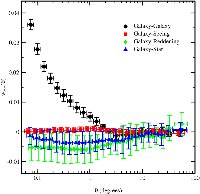
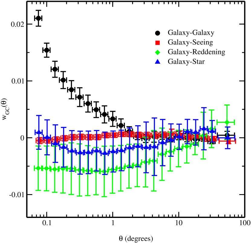
Figure 11: Large-angle cross-correlation of galaxy density and seeing, reddening and stellar density for the magnitude bins $20\leq r^{*}\leq 21$ (left) and $21\leq r^{*}\leq 22$ (right). The anti-correlation for the reddening and stellar density is due to variations on the scale of the observed area. Since this affects the zero-point for the over-densities, the anti-correlation occurs on all scales.

Figure 11 shows the cross-correlation between the galaxy density and seeing, reddening and stellar density using this method for the faintest two magnitude bins. As with the results in Figure 10, the galaxy-seeing cross-correlation is consistent with zero on all scales for both magnitude bins. The galaxy-reddening and galaxy-star cross-correlations, however, differ significantly from the small scales. This can be understood readily by recognizing that the variation in galactic latitude over the course of the observing area leads to large-scale variations in the reddening and stellar density while the seeing variation is basically a small-angle phenomena. (Since we calculated the expected values for the contaminants independently for each sub-sample in Equation 3.4, these large-scale variations would not factor into those measurements.) As a result, we see a rather flat cross-correlation in the large-angle measurements consistent with zero at the $1.5\sigma$ level. The effect of this cross-correlation is the uniform inflation of the galaxy-galaxy auto-correlation when calculated on large scales, similar to the integral constraint discussed in §10.2.

4 Magnitude System

For the actual angular clustering measurements as well as the cross-correlation tests in §3.4, the magnitude cuts have been made using the model magnitudes described in §2.1. This choice contrasts with a number of other SDSS papers on the EDR which use Petrosian magnitudes (Petrosian, 1976). Our decision to use model magnitudes for the angular clustering is based on two points. First, while Petrosian magnitudes are appropriate for relatively bright galaxies, they are not intended for stars. At model magnitudes brighter than $r^{*}=19$, stars are roughly 0.05 magnitudes fainter in Petrosian magnitudes than in PSF magnitudes (there is, of course, no significant disagreement between model magnitudes and PSF magnitudes in this range). At fainter magnitudes, this disagreement blurs into considerable scatter between the two magnitude systems, with disagreements as large as half a magnitude fainter and 0.1 magnitudes brighter. Clearly, since we do not strictly separate between galaxies and stars, Petrosian magnitudes are not a proper tool for separating our sample into different magnitude cuts. Additionally, for galaxies, there is a general disagreement between the model and Petrosian magnitudes, with the Petrosian magnitude for a given object fainter by roughly 0.15 magnitudes, but with a much larger scatter than for the stars. (these large errors are not due to failures in calculation, but an artifact of the occasionally very large apertures dictated by the Petrosian method).

As a result of these differences, applying the same numerical magnitude cuts using Petrosian and model magnitudes results in a slightly larger amplitude for $w(\theta)$ from the Petrosian sample, relative to the model magnitude selection. For the brightest three magnitude slices, the measurements are just within the $1\sigma$ errors on the smallest scales, while for the faintest bin, they are only within the $2\sigma$ errorbars. The cross-correlations with seeing and reddening are consistent with zero on all angular scales within $1\sigma$ errors. The galaxy-star cross-correlation is roughly a third stronger for the faintest magnitude bin using the Petrosian magnitude cut, but still considerably smaller than the galaxy auto-correlation. Switching to Petrosian magnitudes has no effect on the cross-correlation with sky brightness. On whole, similar cuts on seeing and reddening would appear to suffice for galaxies selected using Petrosian magnitudes, but, again, these magnitudes may not be appropriate for faint objects, particularly those which are not easily separated into galaxy and star types.

5 Masks

In addition to making the cuts on seeing and reddening described in §3.4.1 and §3.4.2, we also mask out all of the stars in the field that have saturated centers, including a rectangular area around the star large enough to encompass any diffraction spikes. Similarly, we mask out two thin regions ($\sim 15^{\prime\prime}$ wide) running the length of the data set where the data processing pipeline flagged nearly all of the objects as saturated due to a bad CCD column. As described later in §7.3, poor telescope collimation caused the PSFs in scanlines 1 and 6 to be noticeably worse than those in the central scanlines (this problem has since been corrected so will not affect any subsequent data). To analyze the possibility of a difference between the central and outer scanlines, we also consider a more restrictive mask that excludes scanlines one and six from each strip.

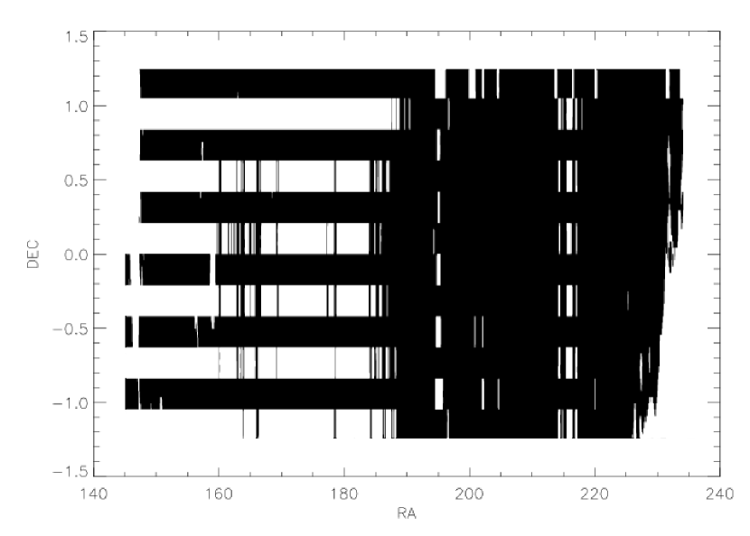
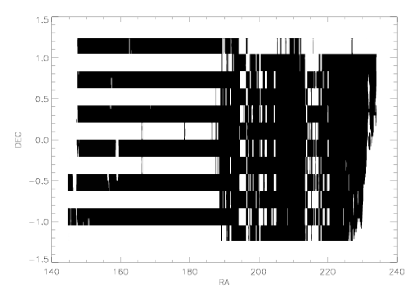
Figure 12: The left panel shows the survey area in the limit that the seeing was better than $1^{\prime\prime}.75$ and reddening better than 0.2 magnitudes, as appropriate for objects brighter than 21 in $r^{\prime}$. The right shows the same, but with the requirement that the seeing was better than $1^{\prime\prime}.6$. This mask was applied to the faintest magnitude bin ($21\leq r^{*}\leq 22$).

Masking out the regions of substandard seeing makes the largest cut in our data (Figure 6), taking out approximately 26% (24%) of the total (central) area for the bright mask (seeing better than $1^{\prime\prime}.75$); the faint mask (seeing better than $1^{\prime\prime}.6$) removes 35% (31%). Imposing our cut on reddening claims roughly another 2%. Finally, the area lost to bright stars is .05% of the total area and the two saturated CCD columns mask another 0.35%. After combining these masks into one unit and eliminating overlaps among the different masks, the total area lost to masks is 28.5% (26.8%) of the total (central) area in the bright mask and 37.9% (33.7%) for the faint mask. The effect of the masks, excluding the bright star masks, are shown in Figure 12.

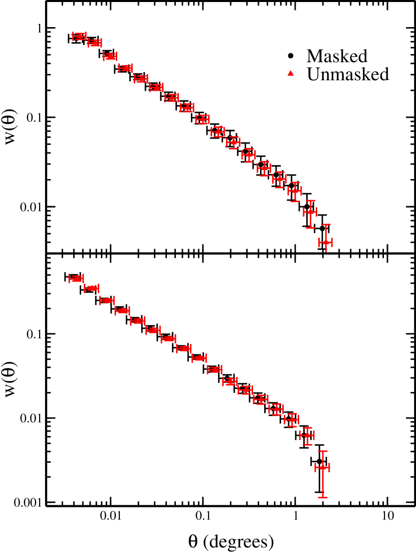
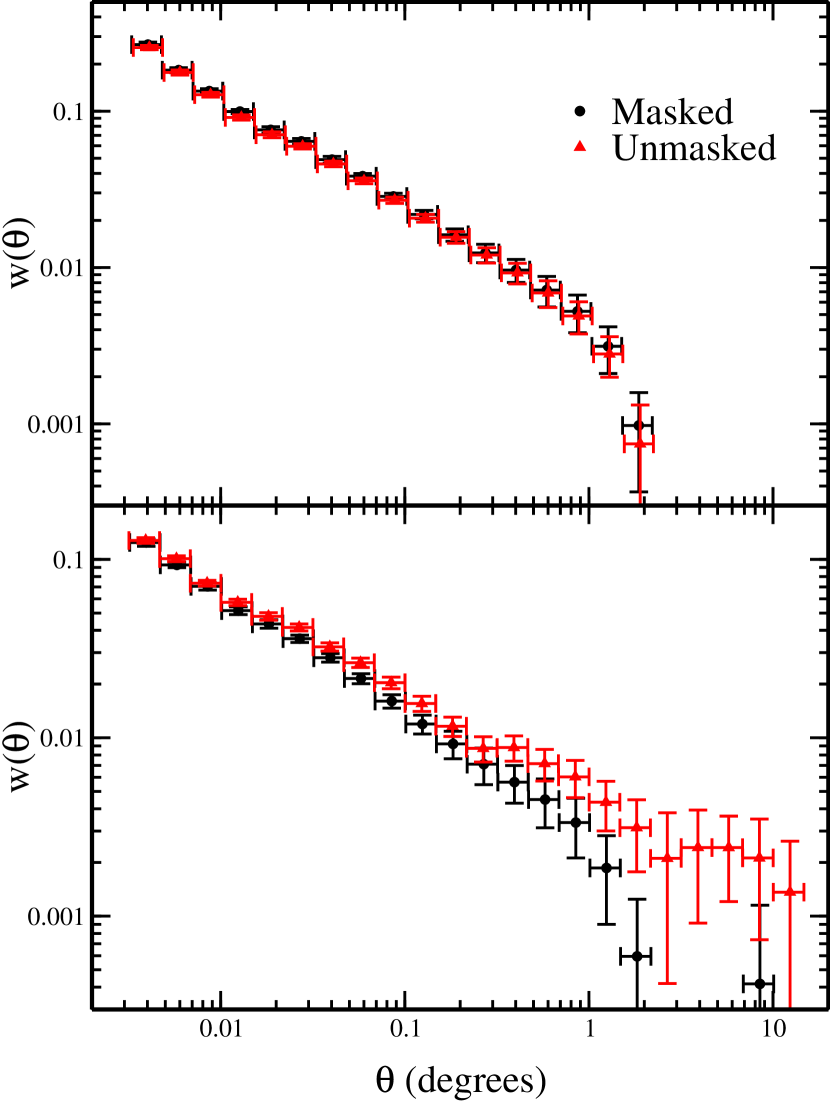
Figure 13: Comparisons of the masked and unmasked measurements of $w(\theta)$ for the four magnitude bins. The left panel shows the $18\leq r^{*}\leq 19$ (upper) and $19\leq r^{*}\leq 20$ (lower) bins and the right panel shows the $20\leq r^{*}\leq 21$ (upper) and $21\leq r^{*}\leq 22$ (lower) bins.

Figure 13 shows a comparison of the masked and unmasked $w(\theta)$ measurements for the four magnitude bins. In general, the effect of the mask on the auto-correlation is quite minimal. This does not hold true, however, for the faintest magnitude bin, where significant departures from the expected power-law shape can be seen, coinciding with our expectations of variations on the scanline-scale due to cross-correlation with seeing.

6 2-D Auto-Correlations

For a further check on the performance of the mask and the data, we can break our auto-correlations into two dimensions, splitting the angular separation between a given pair of objects into its components along the scanline and orthogonal to the scanline ($\alpha$ and $\delta$ in our case, since our area parallels the Celestial equator). If we have variations in density correlated with the interlaced scanlines, then we should see striping along the scan direction.

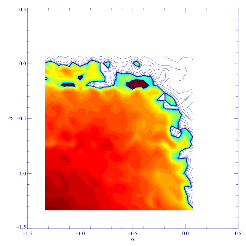
Figure 14: Galaxy auto-correlations (positive contours are filled and negative are in wire-frame) for the $21\leq r^{*}\leq 22$ magnitude bin with the angular separation broken into its component parts along the $\alpha$ and $\delta$ axes. All four magnitude bins show good symmetry in the scanwise and orthogonal directions, indicating sufficient masking of bad regions. X and Y axes are the logarithms of the angular bin in degrees in the $\alpha$ and $\delta$ directions, respectively.

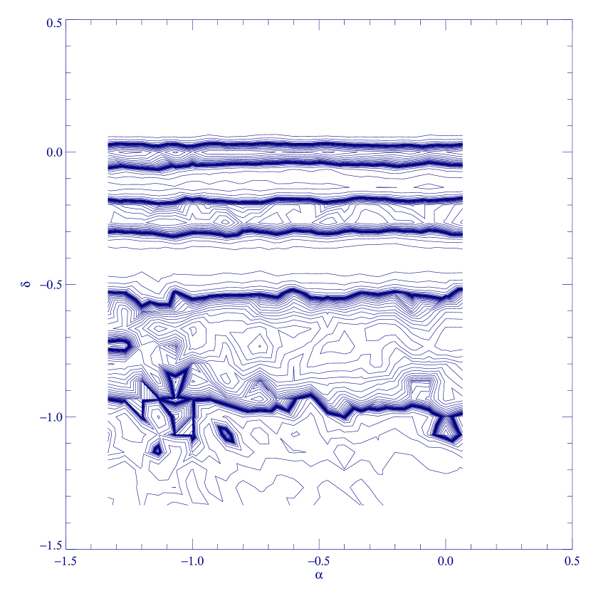
Figure 15: Residual difference between the masked and unmasked 2-D galaxy auto-correlations for $21\leq r^{*}\leq 22$. The brighter three bins have minimal structure along the scanlines but the faintest bin shows significant banding on the scale of the scanlines, a clear sign that the mask is necessary to avoid contamination.

As shown in Figure 14, we recover a radially symmetric auto-correlation for the faintest magnitude bin (as well as the three brighter bins), confirming that our sample is uniform over the transitions between scanlines; the slightly rectangular appearance in the plot contours is an artifact of the angular binning. We can also use this measurement to demonstrate how the mask improves the auto-correlations. In Figure 15, we show the results of subtracting the auto-correlation for the faintest bin calculated without the mask from the plot shown in Figure 14. For the three brightest magnitude bins, there is no obvious striping due to variations in the galaxy density between scanlines, but we do see a rather modest uniform offset, which is perhaps due to a decrease in stellar contamination for the masked sample. This is not true for the faintest magnitude slice, however, which shows exactly the striping in the unmasked measurement we predicted for variations in the galaxy density between strips. The mask removes this behavior to the limit of our ability to measure it with this test. The same exercise can be repeated for the stellar population with similar results, albeit with less visually impressive results as there is no inherent signal due to clustering.

7 Camera Column Variations

The previous sections dealt with errors that were the result of external effects on the galaxy data set and we were able to set limits on the associated contaminants that would produce a uniform galaxy catalog across the area of the survey to the best of our ability to measure. In addition, however, uncorrected variations in sensitivity across the imaging camera could lead to false correlations. We test for such effects in this section.

7.1 Intra-Column Variations

The first check is that the CCDs that create each of the camera columns has a uniform depth of field. Variations in PSF due to telescope collimation errors or the like across a given detector could, if not taken into account, lead to artificial density variations in object densities and classifications. Improvements in the data processing pipeline have reduced the effect of this on our star/galaxy classification and photometry below our ability to detect it.

To demonstrate this, we use a finer pixelized version of the data described in §3.4 (cells with sides $\sim 0.01^{\circ}$ long instead of $\sim 0.04^{\circ}$, using the masks described in §5) and compare the fractional over-density for a given cell $i$, $\delta_{i}$ as calculated in Equation 7, in each column to a series of over-density gradients ($\Delta_{i}$) across the chip in the $\delta$ direction. We choose stellar density rather than galaxy density as it should be free of actual clustering due to large scale structure. The over-density gradients are constructed as sines and cosines:

$$\Delta_{i,n|m}=\left\{\begin{array}[]{c}A_{n}\cos\left(\frac{2\pi n}{\delta_{L}}\bar{x}_{i}\right)\\ B_{m}\sin\left(\frac{2\pi m}{\delta_{L}}\bar{x}_{i}\right)\end{array}\right\}$$ (11)

where $\bar{x}_{i}$ is the mean declination for cell $i$, $\delta_{L}$ is the width of the column ($\sim 2.52^{\circ}$), $A_{n}$ and $B_{m}$ are chosen such that

$$\sum_{i}\Delta_{i,n|m} = 0$$ (12)

$$\sum_{i}\Delta_{i,n|m}\Delta_{i,n|m} = 1,$$ (13)

and $A_{n}=0$ for $m>0$ and vice-versa. We define

$$C_{n|m}\equiv\frac{1}{N}\sum_{i}\delta_{i}\Delta_{i,n|m},$$ (14)

where $N$ is the number of pixels and $C_{n|m}=0$ provided that there is no correlation between the two over-densities. This is effectively decomposing the projection of the stellar over-densities along the scan direction into Fourier cosine and sine modes.

Since we have 216 cells in the declination direction, we can let $n$ and $m$ vary from 0 to 108 and still resolve the variations in $\Delta_{i,n|m}$. Calculating the sum in Equation 14, we should detect any fundamental variations orthogonal to the scanlines. We find, however, that the whole of the data satisfies equation 14 to within $2\sigma$ of the Poisson errors for all 216 gradients in all four magnitude bins.

We can also repeat this exercise for each scanline independently. Here, our maximum value for $n$ and $m$ is reduced to $9$ and $\delta_{L^{*}}=\delta_{L}/12$. Once again, we do not observe any statistically significant non-zero elements of $C_{n|m}$ for any of the scanlines in either column, indicating that we are not producing correlations due to differential response in the camera columns.

7.2 Cross-Column Correlations

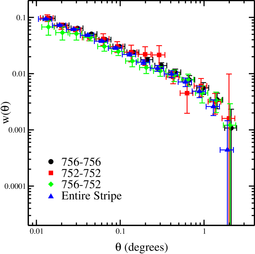
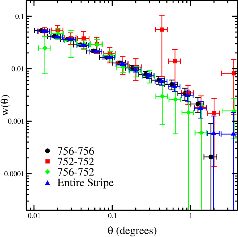
Figure 16: Galaxy auto-correlations for each of the runs in the stripe and the cross-correlation between the runs as compared to the auto-correlation for the whole stripe for the $20\leq r^{*}\leq 21$ (left) and $21\leq r^{*}\leq 22$ (right)

As a further check on column-to-column variations, we calculated the galaxy auto-correlation using the sub-sample method within each of our runs independently of the other, as well as the cross-correlation between the galaxies in each of the runs. If our calibrations and sensitivities are consistent from run to run, each of these should be consistent with the measurement we make from the entirety of the stripe. The results of this measurement using the pixelized data set from §7.1 and the sub-sampling error method from §3.4 for the two faintest magnitude bins are in Figure 16. In general, they confirm that our system is behaving as we would hope. There is some spurious signal from the auto-correlation in Run 752 around the scale size of a scanline, but that is likely to be due to the fact that most of that run is masked for the first half of the range in right ascension (see Figure 12).

7.3 Central Scanlines vs. All Scanlines

The SDSS camera provides an extremely flat depth of field, so as to make the observation of objects as they drift across the field as uniform as possible. However, as mentioned above, at the time that these data were taken, the telescope was not properly collimated (this has since been corrected). The result was that the PSFs in the outer two scanlines of each run were noticeably poorer than the central ones, particularly scanline 6 in each run. This, in turn, made calculation of the photometric calibration more difficult in those scanlines.

As mentioned previously, the photometric calibration is generally done by setting photometric zeropoints based upon secondary stars observed by the PT in the region imaged by the main camera. The uniformity of this calibration can be checked by comparing the magnitudes of objects in the $\sim 2^{\prime}$ overlap region between adjacent scanlines. In $r^{*}$, the median photometric zeropoint offset, as determined from photometry of stars, is less than 2% for all scanlines of data except for scanline 6, which shows deviations of up to 5%. For galaxies with $r^{*}<19$, we find that the rms difference between model magnitudes in the two runs in the overlap is typically 0.04 mag in $r^{*}$, about 30% larger than the nominal photometric errors would imply.

Clearly, this sort of calibration error could potentially lead to a change in the galaxy density for a given magnitude range in those camera columns compared to the central scanlines, although such a variation is not apparent from the galaxy density plots in Figure 3. We tested this possibility by excluding the outer scanlines and re-calculating the cross-correlations and auto-correlations from §3.4. In general, the central scanlines were somewhat less sensitive to systematic contaminants than the whole of the data, but it appears that adding the outer scanlines does not effect the resulting auto-correlation.

8 Limber Scaling Tests

To test the consistency of the $w(\theta)$ measurements and check whether the variations in $w(\theta)$ are due to intrinsic clustering effects rather than systematic errors, a magnitude scaling test using the relativistic form of Limber’s equation was applied to the results. Since $w(\theta)$ is given by the two-dimensional projection of the spatial clustering function $\xi(r)$, the $w(\theta)$ measurements will be scaled according to the depth of the survey (Peebles, 1980).

With a model for the redshift distribution $dn/dz$, we can scale the measurements of $w(\theta)$ in disjoint magnitude slices to the same depth. This method is essentially identical to the one employed in the APM survey (Maddox et al. 1996), described there in greater detail. We assume the same two-slope form of $\xi(r)$, with slopes of $\gamma=1.7$ at small angles and $\gamma=3.0$ at large angles, and ignore effects of evolution in $\xi(r)$.

As with the simulated catalogs discussed in §11.1 below, the $dn/dz$ selection function was based on the results of the CNOC2 survey (Lin et al., 1999), which used a parametrized model for the evolution of the galaxy luminosity function. It assumed a standard Schechter function with no evolution in $\alpha$ and fit a linear evolution model for $M^{\star}$ to $M^{\star}(z=0.3)$, which was the mean redshift for CNOC2 galaxies. Calculations were performed for two different cosmologies: a critical-density universe ($\Omega_{m}=1,\Omega_{\Lambda}=0$) and an under-dense model dominated by a cosmological constant ($\Omega_{m}=0.3$, $\Omega_{\Lambda}=0.7$).

Because the commissioning data form a narrow stripe, it does not allow us to accurately calculate $w(\theta)$ at angles larger than $\sim 1^{\circ}$, so we cannot observe the expected break in the power law. The break from power law form should occur at larger angles for fainter magnitudes, which is accounted for in the scaling tests, but we cannot verify this using the commissioning data.

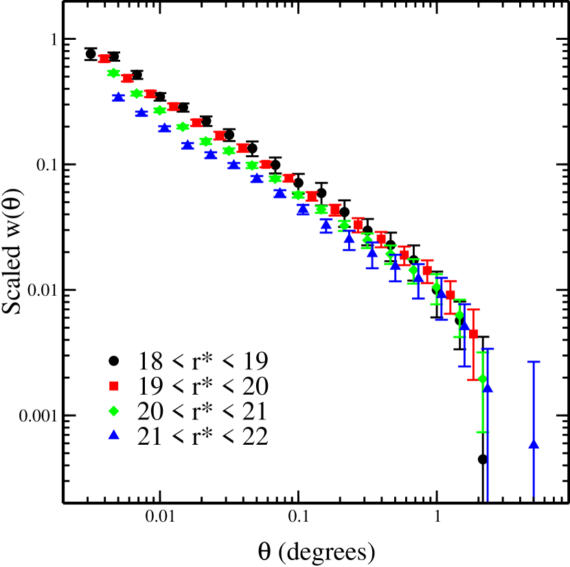
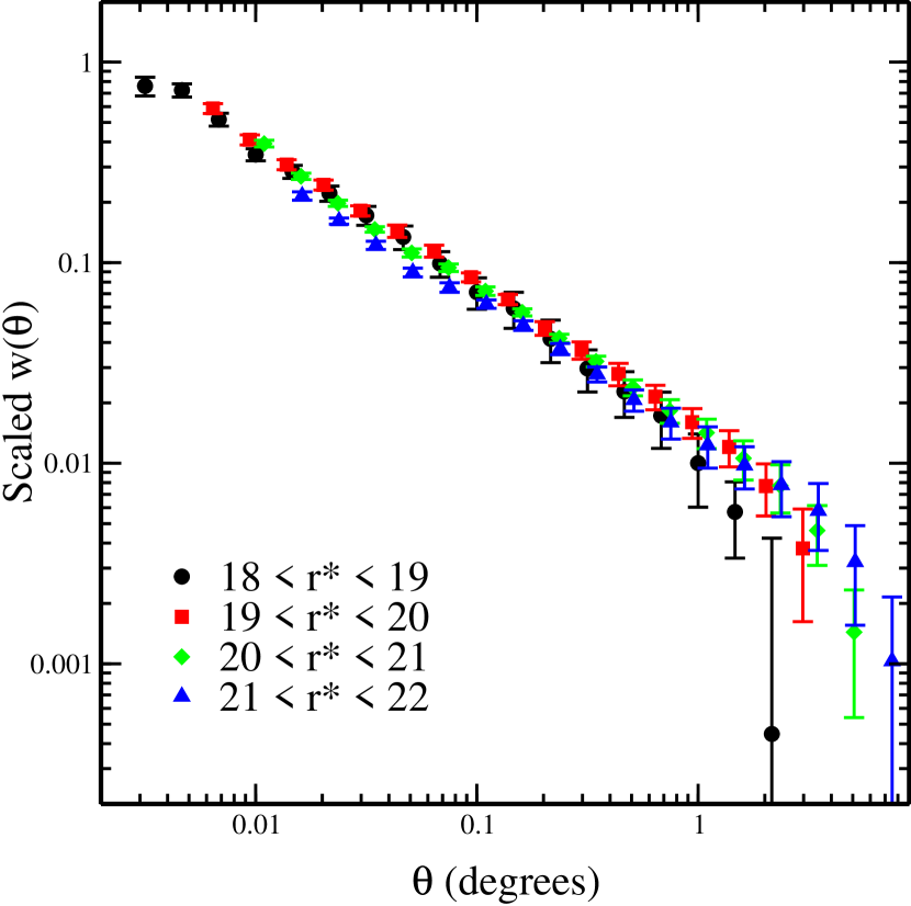
Figure 17: Limber scaling tests for the four magnitude bins assuming a flat, matter-dominated cosmology (left panel) and flat, $\Lambda$-dominated cosmology (right). In both cases, the measurements in the fainter bins have been scaled to the brightest magnitude bin.

As seen in Figure 17, the critical-density calculations show good agreement for the brighter magnitude bins, with progressive worsening for the fainter magnitudes. This does not contradict the APM measurements (Maddox, 1996), since the APM survey had a magnitude limit of $b_{J}=20.5$ and the discrepancy only becomes significant for the faintest magnitude bins, due to the strongly differing size of the volume element at large ($z>~{}0.5$) redshifts between the cosmological models examined.

The lambda-dominated tests show much better agreement across all magnitude ranges. The fact that the scaling tests should support an under-dense, lambda-dominated universe is not surprising, since measurements of $dn/dz$ of faint galaxies (Fukugita et al. 1990) have been known to be incompatible with a critical-density universe for some time.

9 Deblending Tests

As our final source of systematic errors, we consider the possibility of errors in deblending nearby pairs of objects during data processing. Since the data pipeline is automated, the software is required to make decisions as to what is a single object and which are close projections of two distinct objects on the sky.

The expected primary source of deblending problems for the magnitude range we are considering is the combination of two distinction objects which cannot be successfully separated. This can happen under a number of circumstances, most notably seeing variations that blur the object images to the point where even pairs of morphologically simple galaxies cannot be clearly separated. Of course, since we are interested in extended objects, we are more sensitive to these errors than we would be if we were only interested in stellar objects. We have the additional concern that the objects causing this sort of error need not be in our magnitude cut, but rather could be stars or galaxies in different magnitude bins.

The primary effect of this error is on the smallest angular scales, where we expect to see a suppression of the number of pairs of objects, as multiple objects in high density regions are interpreted as single objects. This effect can then propagate to larger angles due to the expected high correlation between angular bins. Likewise, since we will have mis-counted the number of objects, our estimation of the number density of objects on the sky could be significantly skewed, resulting in a suppression of the auto-correlation signal similar to an integral constraint (as discussed in §10.2) on all angular scales.

9.1 Input Catalogs

Since we do not know a priori what the nature of the deblending errors would be in our data, we need a training set of perfectly resolved data that could then be manipulated to simulate various deblending failures. For this purpose, we use mock catalogs (described in section §11.1) that generated for the measurement of the $w(\theta)$ covariance matrix. Since we expect that the rate of deblending error is highly dependent on the density of objects on the sky, we concentrate on the mock catalogs simulating the faintest magnitude bin. The other three magnitude bins as well as a randomly distributed set of points with projected density approximately equal to the stars were used to simulate foreground objects that might also cause deblending problems.

9.2 Small-Angle Supression Test

To measure the suppression of the small-angle signal due to deblending errors, we concentrated solely on the possible failure of the deblender to separate close pairs of objects. To simulate the efficacy of the deblender, we calculated the separation of all objects within the main sample and the separation on the sky of those objects and objects in the foreground sample. This separation ($\Delta\theta$) was used to generate a probability of being successfully separated using a sigmoid function of the form

$$P(\Delta\theta)=\left(1+e^{-(\Delta\theta-\sigma_{c})/\sigma_{s}}\right)^{-1},$$ (15)

where $\sigma_{c}$ represents the separation at which half the objects are successfully deblended and $\sigma_{s}$ controls the slope of the likelihood. Applying this treatment to the data resulted in a sample in which the likelihood of close objects being successfully deblended decreases according to their relative separations. We let $\sigma_{c}$ vary from 0” to 5” and $\sigma_{s}$ from 0 to 1.25 ($\sigma_{s}=0$ indicating a step-function at $\Delta\theta=\sigma_{c}$), calculating $w(\theta)$ for each combination and comparing the result to the observed suppression in the data:

$$\delta w(\theta)\equiv\frac{w_{T}(\theta)-w_{D}(\theta)}{w_{T}(\theta)},$$ (16)

where $w_{T}(\theta)$ is the value expected from the template and $w_{D}(\theta)$ is the measurement with deblending errors. For the actual data, we made the assumption that the “true” $w(\theta)$ is well-described as a power law; Connolly et al. (2001) gives the parameters for this fit. Treating this power law as the $w_{T}(\theta)$ for the real data, we found the combination of $\sigma_{c}$ and $\sigma_{s}$ that produced residuals similar to the residuals in the data. The best fitting values for $\sigma_{c}$ and $\sigma_{s}$ are 3” and 0.5, suggesting that we cannot trust the deblender to function on this data at better than 95% efficiency for angular scales smaller than $\sim 6^{\prime\prime}$. In the mock catalogs, this level of deblending errors reduced the number of galaxies by 2.6%, small enough not to have an apparent effect on the overall integral constraint (see §10.2).

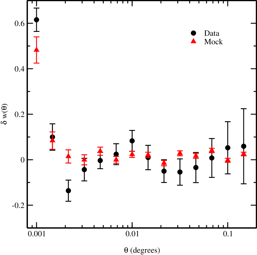
Figure 18: The $\delta w(\theta)$ residuals for the best fitting model of the deblending errors. In both the data and the simulation, aliasing of power and non-zero covariances between angular bins lead to variations which are, however, consistent with zero for angular scales $>6^{\prime\prime}$.

Although the data on angular scales larger than 6” is consistent with a power-law and the mock catalog with the simulated deblending errors is consistent with the template measurement, the residuals plotted in Figure 18 suggest that the lower angular limit on deblender efficiency generates periodic variations in the data. The suspected source of these variations is the aliasing of power into the third angular bin from the first two and the large covariance between the angular bins. These variations are consistent with zero for this measurement, but improvements in the errors due to a large observing area would likely make them discordant. This suggests that future SDSS measurements of $w(\theta)$ will need to take deblender effects into account to avoid misleading signals on all scales. Additionally, one might mitigate these effects by looking at magnitude-weighted angular correlations.

10 Estimators & Biases

Having checked both the internal and external sources of systematic errors which might apply to any angular clustering or photometric work, as well as developing a mask and angular limit to avoid regions where we would have significant systematic errors, we are now ready to address more specific issues related to the measurement of $w(\theta)$ and the associated covariance matrices.

10.1 Estimators

We now turn our attention to the estimators for $w(\theta)$. There are a number of estimators in the literature (Peebles (1973), Sharp (1979), Hewett (1982), Landy & Szalay (1993), and Hamilton (1993)), but we have generally relied on two:

$$\hat{w}(\theta)=\frac{DD-2\langle DR\rangle+\langle RR\rangle}{\langle RR\rangle},$$ (17)

where $DD$ is the number of galaxy pairs in a given angular bin, $\langle RR\rangle$ is the expected number of random pairs for a random catalog of similar density and geometry and $\langle DR\rangle$ is the expected number of cross-population pairs; and

$$\hat{w}(\theta_{\alpha})=\frac{\sum_{i,j}\delta_{i}\delta_{j}U_{i}U_{j}\Theta^{\alpha}_{ij}}{\sum_{i^{\prime},j^{\prime}}U_{i}U_{j}\Theta^{\alpha}_{i^{\prime},j^{\prime}}},$$ (18)

where $\delta_{i}$ is the fractional overdensity in cell $i$ (as given in Equation 7), $U_{i}$ is the fraction of cell $i$ that is unmasked, and $\Theta^{\alpha}_{i,j}$ is 1 if cells $i$ and $j$ are separated by a distance in angular bin $\alpha$ and zero otherwise. This is similar, of course, to the estimator in §3.4, but with a cell size determined by the desired angular resolution and terms to deal with a mask that is independent of the cell size. The estimators in Equations 17 and 18 are identical in the limit of infinitely small cell sizes (Szapudi & Szalay (1998)).

In its simplest form, the first estimator has the advantage in that it can, in principle, probe all of the angular scales in a fixed amount of time. Traditionally the time to perform this calculation goes as $\mathcal{O}(N^{2})$. We can take advantage of the shape of the data area to speed up the calculation, sorting the objects by $\alpha$ and only considering pairs separated by angles less than the largest angular bin.

While this offers an improvement, the large numbers of measurements necessary to calculate the covariance matrices (see §11.1) require a more sophisticated technique. For this calculation, we take advantage of kd-trees ($k$-dimensional data tree structures describing the distribution of the data) to make the calculation run more or less linearly with the number of galaxies. The power of kd-trees for pair counting calculations, as developed by Friedman, Bentley and Finkel (1977), comes in the quick elimination of large fractions of the data, reducing the number of distance calculations for each pair of objects. This is accomplished by recursively subdividing the data area into smaller nodes (generally by splitting along the widest axis of the data area) until sufficient resolution is achieved, one object per node in our case. A search for objects within some radius of a given point in the data area can simply trace back up the data tree until the nodes pass out of its accepted radius, avoiding most of the data in the process. In addition, one can calculate numerous statistics at each node (count, centroid, covariance, etc.) to create an mrkd-tree, improving the ability of the code to determine whether it should progress to the next node to find viable pairs. To make our calculations, we used a version of the mrkd-tree code (the NPT code) developed by Gray & Moore (2001). The nature of this code makes it extremely fast for scales $\leq\sim 0.2^{\circ}$, but it bogs down for larger angles such that we prefer to use the pixelized version of the code for those scales.

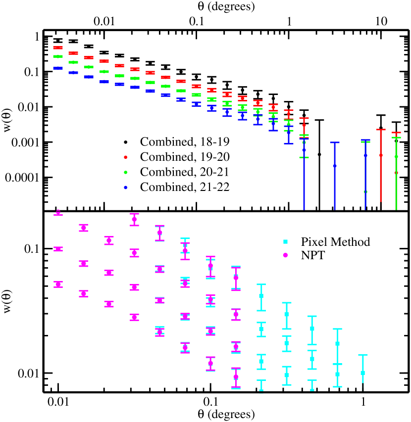
Figure 19: The upper panel shows the results of $w(\theta)$ measurements using the estimator in Equation 17 for angular scales less than $0.15^{\circ}$ and the estimator in Equation 18 for angular scales larger than $0.04^{\circ}$. The lower panel shows the agreement between the two estimators in the overlapping angular bins.

The virtues of the second estimator are more apparent on large scales, where the number of pixels needed is much less than the number of galaxies. It also has the advantage of a more natural generalization to dealing with correlations between continuous phenomena (e.g., galaxy density and seeing), allowing us to use it for the cross-correlations in §3.4. We have verified that these two methods give comparable measurements of $w(\theta)$ over two decades of our angular bins (at 6 bins per decade in degrees), although in the full measurement and calculation of the errors we restricted the angular overlap region to four bins. By approximately matching the processing time for the two codes, we used the pair counting estimator for scales from $0.001^{\circ}$ to $0.15^{\circ}$ and the pixelized version for scales from $0.04^{\circ}$ to our upper limit at $14.7^{\circ}$. This gives us 26 angular bins, 14 for the pair counting estimator and 18 for the pixelized estimator. Figure 19 shows the results of combining these two estimators to give the full range of angular measurements, as well as the measurements for each technique in the overlap range. As expected the two methods agree very well and the transition is quite smooth.

10.2 Integral Constraint

Regardless of the method used, all estimators for $w(\theta)$ are plagued by the “integral constraint”. Again, there has been considerable work done on this problem in the literature (e.g. Peebles 1980, Landy & Szalay 1993, Hamilton 1993, Bernstein 1994, Tegmark et al. 1998, Hui & Gaztañaga 1999, Szapudi et al. 1999). The central problem in these calculations lies in the fact that the calculation of the mean number density ($\bar{n}$) for a given cell is not the “true” number density, but only an estimator thereof ($\hat{\bar{n}}$) based upon a finite number of galaxies and cells. This estimator enters into the estimator of the auto-correlation $\hat{w}(\theta)$ in a non-linear fashion and generally tends to suppress our estimate of the “true” $w(\theta)$. We will explicitly give the corrections only for the pixelized estimator (Equation 18), but the treatment for the particle-based estimator (Equation 17) follows similar lines.

10.2.1 Bias Correction

Since our estimator for $\hat{\bar{n}}$ enters in the calculation of the over-density, we have to re-define $\hat{\delta}$ as

$$\hat{\delta_{i}}\equiv\frac{n_{i}-\hat{\bar{n}}}{\hat{\bar{n}}}=(\delta_{i}-\alpha)(1-\alpha+\alpha^{2}-\ldots),$$ (19)

where $\delta_{i}$ is the true overdensity for pixel $i$ and we have parameterized our bias due to using a finite sample with $\alpha$,

$$\alpha\equiv\frac{1}{N}\sum_{i}\delta_{i},$$ (20)

where $N$ is the number of pixels in the survey area. Plugging Equations 19 and 20 into 18, it can be shown that our estimator for $w(\theta_{\beta})$ has an expectation value of (see e.g. Hui & Gaztañaga 1999 for details)

$$\left\langle\hat{w}(\theta_{\beta})\right\rangle=w(\theta_{\beta})-\frac{1}{N^{2}}\sum_{i,j}w(\theta_{i,j})-\frac{2}{N^{2}}\sum_{i,j,k}w_{3}(\theta_{i,j,k})W_{ij,\beta}+w(\theta_{\beta})\frac{3}{N^{2}}\sum_{i,j}w(\theta_{i,j}).$$ (21)

where shot noise is excluded (which can be shown to contribute negligibly to the integral constraint bias), and where $W_{ij,\beta}$ is our window function,

$$W_{ij,\beta}=\frac{\Theta^{\beta}_{ij}U_{i}U_{j}}{\sum_{i^{\prime},j^{\prime}}\Theta^{\beta}_{i^{\prime},j^{\prime}}U_{i}U_{j}}.$$ (22)

The above expression for $\left\langle\hat{w}(\theta_{\beta})\right\rangle$ keeps all terms that are first order in $N^{-2}\sum_{i,j}w(\theta_{i,j})$ (assuming $w_{3}$ is related to $w$ in the usual hierarchical fashion), which can be regarded as the small parameter of our expansion. Note that this expression does not assume $w(\theta_{\beta})$ is itself small. The second term on the right hand side of Equation 21 is what Peebles (1980) originally derived for integral constraint correction.

To estimate the integral constraint correction, we use the hierarchical relation to approximate the $w_{3}(\theta)$ term as

$$-\frac{2}{N^{2}}\sum_{i,j,k}w_{3}(\theta_{i,j,k})W_{ij,\beta}=-w(\theta_{\beta})\frac{2c_{12}}{N^{2}}\sum_{i,j}w(\theta_{i,j}),$$ (23)

where $c_{12}\equiv w_{3}/w_{2}$ is the hierarchical amplitude. Bernardeau (1994) gives the value of this parameter as $c_{12}=68/21+\gamma/3$, where $\gamma$ is the logarithmic slope of the variance and galaxy biasing is ignored. For reasonable values of $\gamma$, this gives $c_{12}\sim 2$. Gathering terms, this gives us our correction ($\Delta\hat{w}(\theta)$):

$$\Delta\hat{w}(\theta_{\beta})\equiv\left\langle\hat{w}(\theta_{\beta})\right\rangle-w(\theta_{\beta})=\left(1+(2c_{12}-3)w(\theta_{\beta})\right)\frac{1}{N^{2}}\sum_{i,j}w(\theta_{i,j}),$$ (24)

We note that the $w_{3}(\theta)$ term does not in fact contribute significantly to the bias on large scales (where the bias is most important), and so the approximations made above do not unduly affect our estimate of $\Delta\hat{w}$ .

Note that this expression contains $w(\theta)$ and not the estimator $\hat{w}(\theta)$ that we have calculated. However, since the sums involved in Equation 24 are suppressed by a factor of $1/N^{2}$, the total amplitude of the correction is quite small compared to the value of $\hat{w}(\theta)$ on most scales. This means that the error that we would make by substituting the estimator values for $w(\theta)$ into Equation 24 should also be quite small. Even if this is not quite the case for all scales, we can note the amplitude of the correction to $\hat{w}(\theta)$ and disregard those measurements where the correction is a sizable fraction of the original estimator. This will come into play in the next section when we consider the applicability of the various error calculations for the estimators.

10.2.2 Magnitude of the Bias Correction

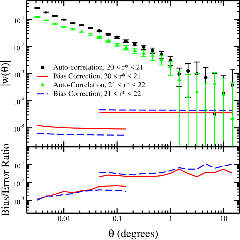
Figure 20: Comparison of the galaxy auto-correlation and its errors to the integral constraint bias correction suggested by equation 24. The different bias correction levels are due to the difference between the number of pixels and number of objects in the large-angle and small angle techniques, respectively. The lower panel gives the ratio of the bias correction and the error on $w(\theta)$.

In Figure 20, we plot the integral constraint bias suggested by equation 24 for the faintest two magnitude bins, comparing them to the auto-correlation and the error on the auto-correlation as determined using the simulations described in §11.1. The difference between the number of objects and pixels used in the estimators from Equations 17 and 18, respectively, lead to different integral constraint corrections on small and large angular scales. In all cases, however, the magnitude of the integral constraint correction remains very small relative to the magnitude of $w(\theta)$ suggesting that our approximation of $w(\theta)$ by $\hat{w}(\theta)$ is fairly well justified.

11 Error Calculation and Correlation

As with any measurement, the calculation of the auto-correlation is only the first step; equally important is the determination of the error matrix. While the Fourier modes in the density field are expected to evolve independently (in the linear approximation), a given angular bin will sample a combination of those modes. This demands that we calculate the correlations between angular bins as well as the standard diagonal elements of the covariance matrix if we want to be able to use this measurement in a meaningful way. Of course, we have to find a method of error calculation that can be practically and reliably applied over more than three decades in angular scales. Unfortunately, there is no single method of error calculation that can do so with the data available alone. Rather, we use simulations to provide us with multiple realizations for error calculation and then check those errors against less preferred data-based methods. Likewise, on large scales, we check the simulation covariances against those calculated from the data under the assumption of Gaussianity. The next four sub-sections outline each of the methods and present examples of the respective covariance matrices.

11.1 Errors from Simulations

The mock catalogs were generated using a new algorithm (Scoccimarro & Sheth 2001) called PTHalos. PTHalos works in two steps, first it generates the large-scale dark matter distribution using second-order Lagrangian perturbation theory (2LPT), which reproduces the correct two and three-point statistics at large scales, and approximates four-point statistics and higher (Moutarde et al. 1991; Buchert et al. 1994; Bouchet et al. 1995; Scoccimarro 2000) very well. The second step builds up the small-scale correlations using the amplitude of the 2LPT density field to determine the masses using the algorithm in Sheth & Lemson (1999) and positions of halo centers, and then distributing particles around the halo centers with NFW profiles (Navarro, Frenk & White 1997). Thus in PTHalos, the large-scale correlation function are the result of the perturbative growth of structure, whereas the small-scale behavior is due to the internal structure of virialized halos. In addition, a “galaxy” distribution can be generated in PTHalos by specifying how many galaxies populate halos of a given mass. Thus, it is possible to design “galaxy” distributions which approximate the observed statistics; for this purpose, we use a similar grid of models to those in Scoccimarro et al. (2001).

The advantage of this method is that it approximates very well the fully non-linear, and thus non-Gaussian, evolution of structure in a very small fraction of the time and cost of a full $n$-body simulation; PTHalos takes about 10 minutes on a DEC Alpha to generate a mock catalog for the four magnitude bins used in this paper that would otherwise cost several expensive hours of CPU. Given the uncertainty involved in modeling galaxy biasing, the approximate nature of PTHalos distributions is a small price to pay in exchange for speed. In particular, the increase in speed means we can run many (of the order of a hundred) realizations of the survey area, and compute errors and covariance matrices for the clustering statistics from a Monte Carlo pool. Therefore, our errors automatically take into account the non-Gaussianity of the galaxy distribution, cosmic variance, shot noise, and the geometry of the survey.

The catalogs are constructed from parent 2LPT simulations containing 54 million particles that correspond to a $\Lambda$CDM model ($\Omega=0.3$, $\Omega_{\Lambda}=0.7$; at $z=0$). The evolution of structure along the past light-cone is done approximately, by tiling boxes with different values of the power spectrum normalization $\sigma_{8}$. A “low redshift” box of side 600 $h^{-1}{\rm Mpc}$ is used for $z<0.4$ with 27 million particles and $\sigma^{\rm mass}_{8}=0.83$. Another box of side 1200 $h^{-1}{\rm Mpc}$ and same number of particles with $\sigma^{\rm mass}_{8}=0.66$ is used for $0.4<z<0.8$.

Galaxies are assumed to populate dark matter halos according to the relation (similar to that in Kauffmann et al. 1999, and Sheth & Diaferio 2001)

$$N_{\rm gal}=0.7x^{0.8}+y^{0.9},$$ (25)

where $N_{\rm gal}$ is the mean number of galaxies per halo of mass $m$. Here $x=m/4\times 10^{12}M_{\sun}/h$ with $x=1$ for $m<4\times 10^{12}M_{\sun}/h$, and $y=m/2.5\times 10^{12}M_{\sun}/h$. In addition, $N_{\rm gal}=0$ for $m\leq 3\times 10^{11}M_{\sun}/h$. Such a biasing relation between galaxies and mass leads to a large-scale bias parameter $b\sim 0.7$.

To generate the galaxy distribution we used the following radial selection functions ($dN/dz\propto z^{2}\psi(z)$):

$$\psi(z)=\frac{A}{z^{a}}\exp(-(z/z_{0})^{2}),$$ (26)

where $A=6.89,28.34,36.42$, $a=1,0.5,0.5$ and $z_{0}=0.21,0.25,0.35$ for magnitudes bin $18\leq r^{*}\leq 19$, $19\leq r^{*}\leq 20$ and $20\leq r^{*}\leq 21$, respectively. For the faintest magnitude bin, we had to use the sum of two selection functions; the first was of the form in Equation 26 with $A=777.35$, $a=0.5$ and $z_{0}=0.21$ and the second with the form

$$\psi(z)=\frac{A}{z^{a}}\exp(-(z/z_{0})^{3}),$$ (27)

where $A=50.025$, $a=0$ and $z_{0}=0.545$. These selection functions are based on the CNOC2 luminosity functions (Lin et al. 1999). The details of this extraction and the conversion to SDSS filters are given along with the inversion of our $w(\theta)$ measurement in Dodelson et al (2001), which also provides an alternate parameterization.

The three-dimensional data is then projected (using different sections of the simulation box without repeating any structures) into an angular stripe of 2.5 by 90 degrees, with the same angular coverage to the actual data from 752-756 runs. In addition to the comparisons between the measurements of $w(\theta)$ in the simulated and real data sets described below, we have also verified that higher-order moments such as skewness and kurtosis match the observed ones to a good approximation (Szapudi et al. 2001).

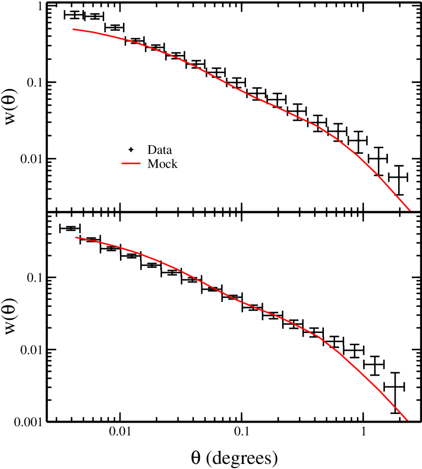
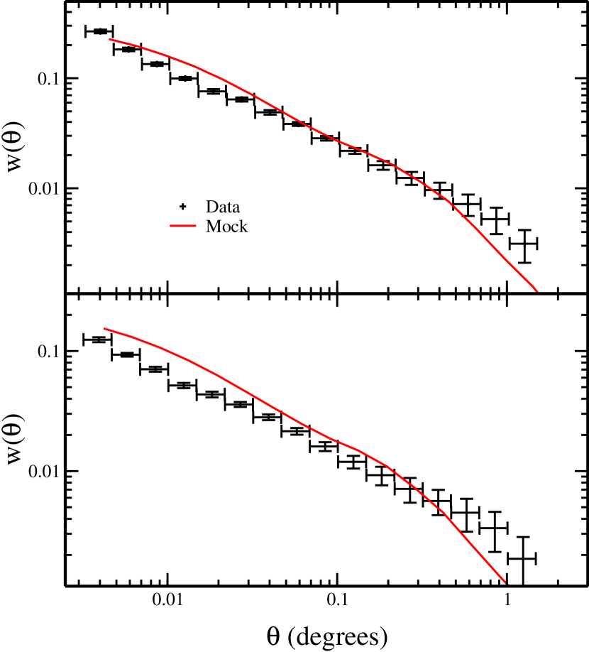
Figure 21: Comparisons of $w(\theta)$ measurements from mock catalogs and data. In the left plot, the upper panel shows the comparison for $18\leq r^{*}\leq 19$ and the lower panel for $19\leq r^{*}\leq 20$. The right plot does the same for $20\leq r^{*}\leq 21$ (upper) and $21\leq r^{*}\leq 22$ (lower).

In Figure 21, we see the direct comparison between the data and the mock catalogs for the four magnitude bins. The “mock” measurement is the mean value of $w(\theta)$ from 100 mock catalogs and the errors come from the diagonal elements of the covariance between these 100 measurements. In general, we see a reasonable agreement between the mock catalogs and the data over the range of angular scales. The one significant discrepancy is in the small angle regime of the $21\leq r^{*}\leq 22$ bin, where the mock catalog over-predicts the auto-correlation compared to our measurement. This may be due to a slight error in the selection function for this magnitude bin or possibly some evolution in the biasing, but should not adversely affect the covariances from the mock catalogs.

11.2 Sub-Sampling Errors

In §3.4, we gave the formalism for calculating the cross-correlation errors from the variance of the mean measurement determined in 35 non-overlapping square sub-samples of the data area. This method works reasonably well for this purpose since we have a reasonable expectation that the sub-sample measurements are not strongly correlated. Since our primary estimators work on $\mathcal{O}(N^{2})$ time, this method also cuts down the processing time for the cross-correlation measurements by a factor of 35.

For the galaxy auto-correlation, we have mixing between physical scales due to projection effects. This means that we have correlations in the sub-samples that are not modeled by Equation 9, resulting in a likely under-estimation of the errors via this method.

11.3 Jackknife Errors

In §3.4.5, we presented the formulae and method for calculating cross-correlation errors on large angular scales using the jackknife approach. We can also apply this method to the calculation of the galaxy auto-correlation errors on our full range of angular scales using the estimator in Equation 17. In order to constrain the 26 angular bins, we use 30 jackknife samplings of the data. In principle, this should generate errors comparable to those from the simulations as this method should not suppress covariances on large scales. In practice, however, the jackknife method appears to generate anti-correlations between angular scales smaller than the regions blocked out for each jackknife sample and the scale size of the blocked-out region (3 degrees in our implementation).

11.4 Gaussian Errors

At the large end of the angular spectrum, we can calculate the covariance matrix under the assumption that the error distribution is Gaussian in nature. In this case, we will be using the pixelized version of the estimator for the auto-correlation (Equation 18). The covariance for such an estimator is generically given by

$$C(\theta_{\alpha},\theta_{\beta}) \equiv \left\langle(\hat{w}(\theta_{\alpha})-w(\theta_{\alpha}))(\hat{w}(\theta_{\beta})-w(\theta_{\beta}))\right\rangle$$ (28)

$$= \left\langle\hat{w}(\theta_{\alpha})\hat{w}(\theta_{\beta})\right\rangle-w(\theta_{\alpha})w(\theta_{\beta})$$

In order to calculate this, we need the covariance for $\delta$,

$$C(\theta_{i,j}) \equiv \left\langle\delta_{i}\delta_{j}\right\rangle$$ (29)

$$= w(\theta_{i,j})+\frac{\delta_{ij}}{N_{i}},$$

where $\delta_{ik}$ is the traditional Kronecker delta, and $N_{i}$ is the number of galaxies in pixel $i$.

Taking this into account for the estimator in Equation 18, the covariance $C(\theta_{\alpha},\theta_{\beta})$ becomes

$$C(\theta_{\alpha},\theta_{\beta})=2\sum_{i,j}W_{ij,\alpha}\sum_{k,l}W_{kl,\beta}\left(w(\theta_{i,k})+\frac{\delta_{ik}}{N_{i}}\right)\left(w(\theta_{j,l})+\frac{\delta_{jl}}{N_{j}}\right),$$ (30)

where we have dropped the fourth order terms which vanish under the assumption that the over-densities have a Gaussian distribution. There are four terms to this sum, but we expect the cosmic variance term (the product of the two auto-correlations) to dominate on large scales, so we will calculate that to the exclusion of the others. Inserting the form of the weight function, we must calculate

$$C(\theta_{a},\theta_{b})=\left(\frac{2}{\sum_{i^{\prime},j^{\prime}}\Theta^{a}_{i^{\prime},j^{\prime}}\sum_{k^{\prime},l^{\prime}}\Theta^{b}_{k^{\prime},l^{\prime}}}\right)\sum_{i,j,k,l}\Theta^{a}_{ij}\Theta^{b}_{kl}w(\theta_{i,k})w(\theta_{j,l});$$ (31)

a calculation which goes as the fourth power of the number of pixels (and is the reason why we do this with pixels instead of by pairs).

In this case both of our technical constraints push us in the same direction toward larger angular scales. First, we pay a heavy penalty for increasing the number of pixels in order to measure smaller and smaller angular scales. Even a modest pixel size of one third of a degree will require on order $10^{13}$ computations. At the same time, we know that the Gaussian approximation will break down at sufficiently small angles, so we have very little motivation for greatly increasing the number of pixels. Indeed, the only reason to do so is to increase the range of angular scales where the Gaussian method reliably overlaps with the errors from the simulation method so as to allow for cross-checking.

12 Method Comparison

Despite the variations between the four error methods with respect to applicable angular range and measurement technique, all of the methods produce covariance matrices that have large off-diagonal elements as expected. Moving beyond this simple observation to a detailed comparison of the covariance matrices for each of the four methods is not a trivial task. As there is no single well-established method for such a comparison, we present a number of tests to compare the shape and amplitude of the covariance matrices. Additional tests of the jackknife and sub-sample methods in comparison to simulated data sets can be found in Zehavi et al. (2001). Due to the large difference in the angular range for the simulation, sub-sample and jackknife errors and the Gaussian errors, we will set the latter aside initially and concentrate on comparing the first three methods. We will finish by comparing the Gaussian covariance matrices to the appropriate parts of the covariance matrices from the simulations using the tools developed in the next sections.

12.1 Correlation Test

Qualitatively, we can compare the shape of the covariance matrices by calculating the correlation matrices for each of the three main methods (simulations, jackknife, and sub-sample). The elements of the correlation matrix ($r(\theta_{\alpha},\theta_{\beta})$) are given by

$$r(\theta_{\alpha},\theta_{\beta})=\frac{C(\theta_{\alpha},\theta_{\beta})}{\sqrt{C(\theta_{\alpha},\theta_{\alpha})C(\theta_{\beta},\theta_{\beta})}},$$ (32)

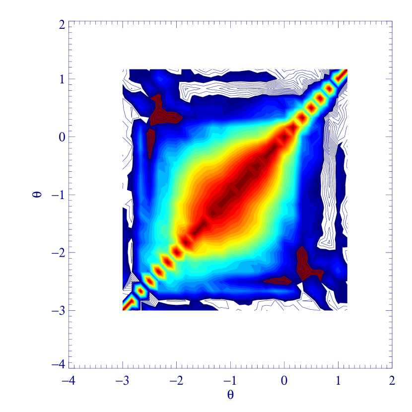
Figure 22: Correlation matrix from simulations for the $21\leq r^{*}\leq 22$ magnitude bin. X and Y axes are the logarithms of the angular bins in degrees. As predicted, the off-diagonal elements of the correlation matrix are significant, regardless of the method used for calculating them.

where $r(\theta_{\alpha},\theta_{\alpha})\equiv 1$ and plotted for the three methods in Figures 22 through 24 for the $20\leq r^{*}\leq 21$ magnitude bin. No matter which set of matrices is to be used for further work (e.g. inverting $w(\theta)$ to recover the three dimensional power spectrum), it is clear that the full covariance matrix must be employed. Likewise, we can see that the sub-sample and jackknife errors have considerably stronger anti-correlations between the largest and smallest angular scales than the simulation correlations. As discussed previously, this anti-correlation for the sub-sample method is an artifact of the assumption that each sub-sample is independent of the others. Likewise, for the jackknife errors, the anti-correlation on the scale-size of the omitted regions strongly suggests that the method is suppressing signal on that scale.

12.2 Diagonal Test

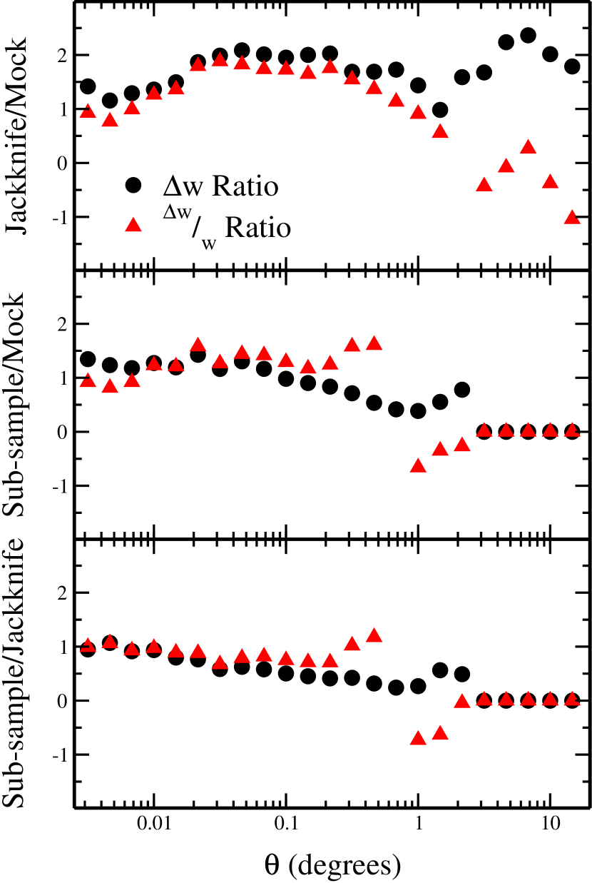
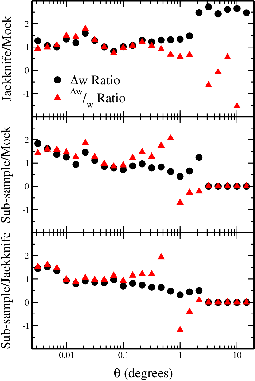
Figure 25: Ratios of $\Delta w$ and $\frac{\Delta w(\theta)}{w(\theta)}$ for the errors calculated using simulations, sub-sample and jackknife techniques for the $18\leq r^{*}\leq 19$ (left) and $19\leq r^{*}\leq 20$ (right) magnitude bins.

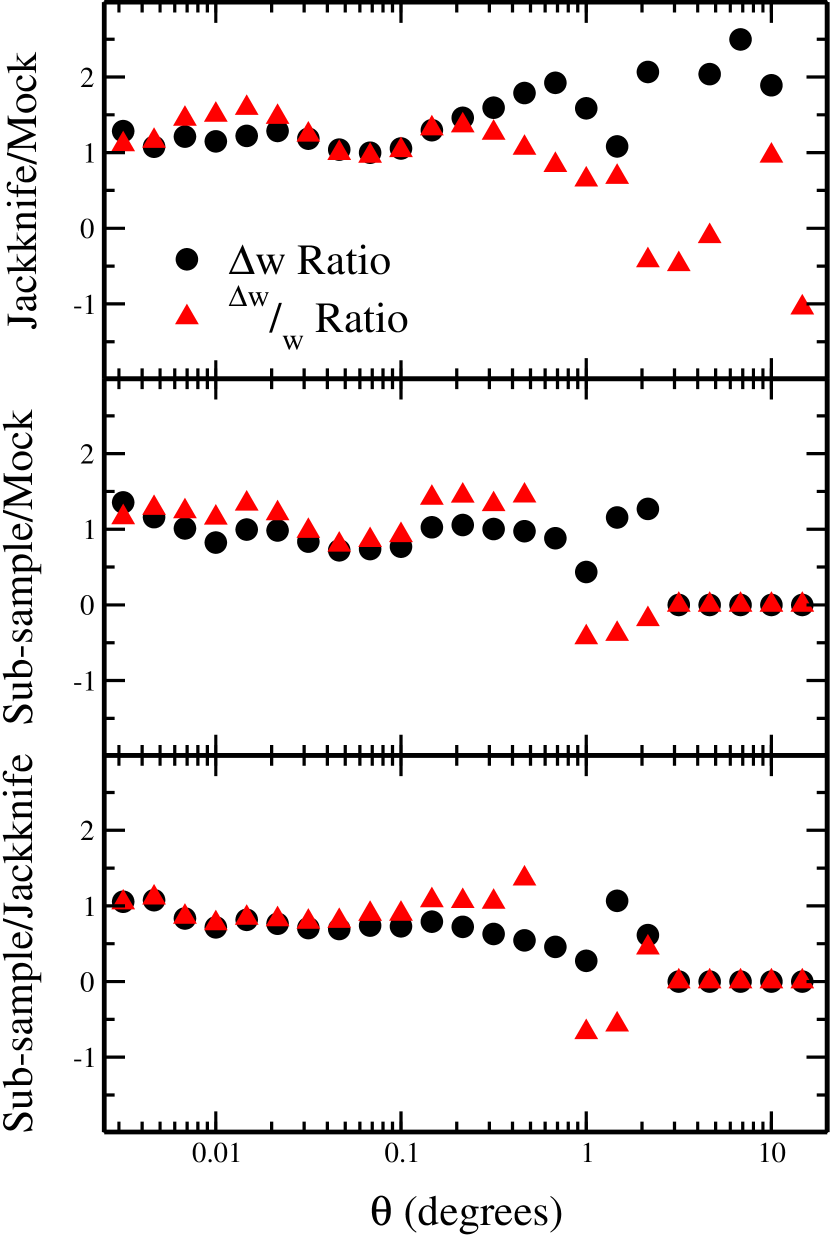
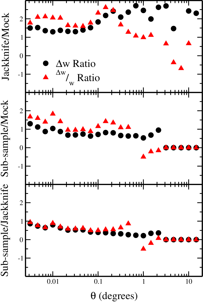
Figure 26: Same as Figure 25, but for the $20\leq r^{*}\leq 21$ (left) and $21\leq r^{*}\leq 22$ (right) magnitude bins.

For a more quantitative comparison, we can examine the diagonal elements of the covariance matrix. Figures 25 and 26 show the ratios of $\Delta w(\theta)$ and $\frac{\Delta w(\theta)}{w(\theta)}$ for the error calculations using the simulations, sub-samples and jackknife methods. Note that, since we are including $w(\theta)$ from each of the methods in the second ratio, a negative value of $w(\theta)$ in only one of the methods can result in a negative ratio, while the first ratio is by definition positive. The diagonals of the covariance matrices for the three methods generally agree to within factors of 1 to 2 for the three methods for the angular scales where they overlap, with considerable scatter as we approach the break in $w(\theta)$. However, it is apparent that the $w(\theta)$ from sub-sample method starts to diverge from that measured from the simulation and jackknife methods at angular scales as small as $0.1^{\circ}$. This makes the sub-sample method a questionable choice except at the smallest scales.

12.3 Product Test

For a more complete comparison of the simulation and jackknife covariance measures, we need to examine the off-diagonal elements. To characterize the contribution of the off-diagonal elements, we calculate $R(\theta)$, where

$$R(\theta_{\alpha})\equiv\left(\prod^{N}_{\beta}|r(\theta_{\alpha},\theta_{\beta})|\right)^{\frac{1}{N}}.$$ (33)

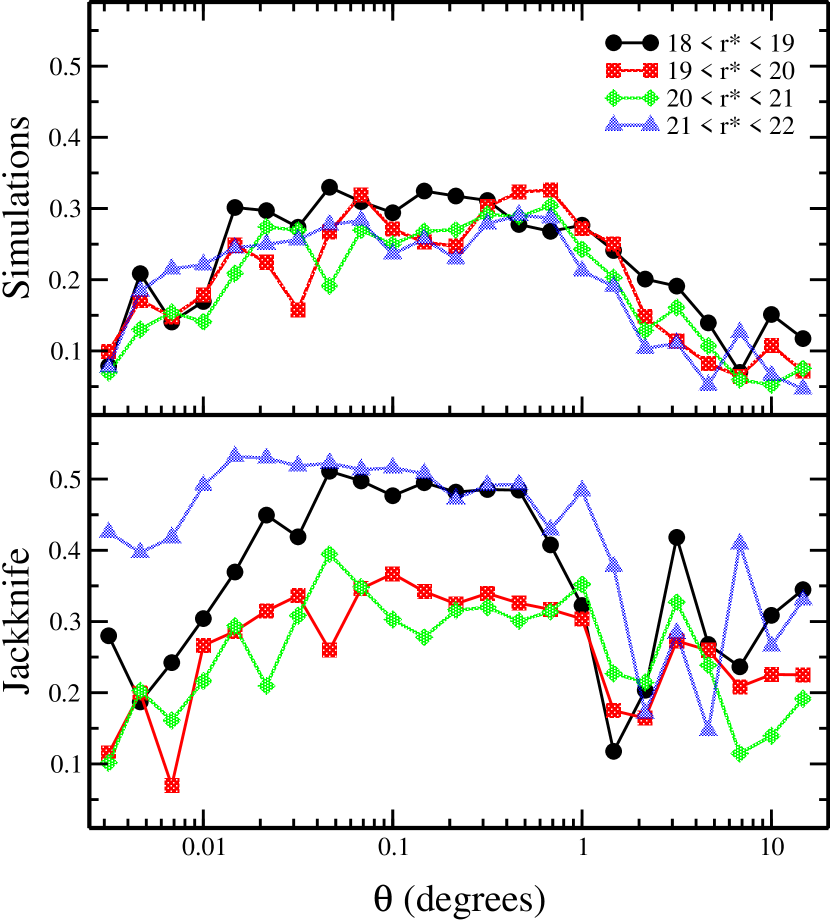
Figure 27: $R(\theta)$ calculations for the simulations and jackknife correlation matrices in all four magnitude bins.

For a perfectly diagonal matrix, this quantity will be zero and would be equal to 1 for perfect correlation (or anti-correlation) between each angular bin. Figure 27 shows the values of $R(\theta)$ for each of the methods in each of the magnitude bins. As expected, both methods show a fairly high degree of off-diagonal correlation by this measure, with the jackknife generally showing larger amplitude off-diagonal elements than the mocks. This confirms our earlier prediction that the jackknife errors are superior to other data-only measurements, but not as well-behaved as the errors from simulations.

12.4 Wishart Likelihood Ratio Test

Alternatively, we can attempt to further quantify the differences between the covariance matrices themselves by calculating their Wishart probabilities. If we measure the same quantity ($w(\theta)$, for instance) on several realizations of statistically similar data, then we expect the measurements to be distributed according to the covariance matrix on that measurement. Likewise, if we calculate the measurement covariance matrix for each realization of the data, then these covariance matrices will be distributed around the “true” covariance matrix for the measurement and the data. If we take the covariance matrix generated from the simulated catalogs to be the “true” covariance matrix for data that is not contaminated by systematic errors, then the probability that the covariance matrix measured on one of the simulated catalogs is drawn from a distribution of the true covariance matrix is given by the Wishart distribution (Wichern & Johnson, 2002),

$$W(C_{S|J}|C_{M})=\frac{|C_{S|J}|^{(N-N_{\theta}-2)/2}e^{-tr(C_{S|J}C_{M}^{-1})/2}}{2^{N_{\theta}(N-1)/2}\pi^{N_{\theta}(N_{\theta}-1)/4}|C_{M}|^{(N-1)/2}\prod_{i=1}^{N_{\theta}}\Gamma((N-i)/2)},$$ (34)

where $C_{S|J}$ is the covariance matrix from either the sub-sample or jackknife methods, $C_{M}$ is the covariance matrix from the simulations, $N$ is the number of mock catalogs, $N_{\theta}$ is the number of angular bins. If the covariance matrix we test fit the distribution perfectly, this would be equivalent to taking $W(C_{M}|C_{M})$, which we denote as $W_{0}$. With this in hand, we can use Equation 34 to perform a likelihood ratio test where

$$q = \frac{W(C_{S|J})}{W_{0}}$$

$$\ln q = \ln W(C_{S|J})-\ln W_{0}\sim-\frac{1}{2}\chi_{S|J}^{2},$$ (35)

where an acceptable $\chi_{S|J}^{2}$ would be roughly equal to the number of independent elements ($k$) of each covariance matrix: $k\equiv N_{\theta}(N_{\theta}+1)/2$.

The application of this test assumes that $w(\theta)$ is distributed normally, and thus the covariance matrix captures all of the information about the variation of $w(\theta)$. While this is not likely exactly correct, we expect it to be a reasonably good approxmation for the bulk of the distribution, with perhaps some disagreement in the tails of the distribution. The effect of this is such that, for very small values of $W(C_{S|J}|C_{M})$, we may not be able to accurately calculate the exact probability, but this should be sufficient for our purposes. In addition to these considerations, we also need to consider the effect of disagreements between the amplitude of $w(\theta)$ in the simulated catalogs and the data (as shown in Figure 21). To isolate the effects of the difference in methods and the difference in measurements, we must apply the sub-sample and jackknife methods to the simulated catalogs and define $C_{S}$ and $C_{J}$ as their respective means. Table 1 gives the results of applying this test to covariance matrices measured using the data and using the mean covariance matrices taken from applying the methods to the set of simulations. The first conclusion to draw from this calculation is that, although the deviation between the jackknife and sub-sample methods is not significant enough to choose between the methods using this test, both methods are reasonably acceptable alternatives to the simulation method if the latter is not available. Secondly, we can see from comparing the first and second sets of columns that the difference in the $w(\theta)$ for the real data and the simulation does lead to some discrepancy between the apparent behavior of each of the methods and the behavior when one uses a common data set.

Finally, we can also generalize Equation 34 to

$$W(C_{S|J}(\Theta)|C_{M}(\Theta))=\frac{|C_{S|J}(\Theta)|^{(N-N_{\Theta}-2)/2}e^{-tr(C_{S|J}(\Theta)(C_{M}(\Theta))^{-1})/2}}{2^{N_{\Theta}(N-1)/2}\pi^{N_{\Theta}(N_{\Theta}-1)/4}|C_{M}(\Theta)|^{(N-1)/2}\prod_{i=1}^{N_{\Theta}}\Gamma((N-i)/2)},,$$ (36)

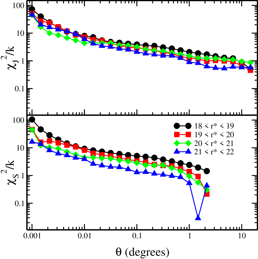
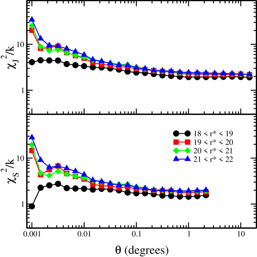
Figure 28: $\frac{\chi^{2}_{S|J}}{k}(\Theta)$ for data (left) and simulation (right) covariance measurements.

where $C_{J|M}(\Theta)$ and $C_{M}(\Theta)$ are the sub-matrices corresponding to the elements of the original covariance matrices where the angular bins involved are both are less than or equal to $\Theta$ and $N_{\Theta}$ is the corresponding number of angular bins. Thus, calculating $\chi_{S|J}^{2}(\Theta)$ allows us to see how the results of the sub-sample and jackknife methods diverge from the simulation covariance as a function of angle. As Figure 28 shows, there is significant deviation at small angles from the relatively low values of $\chi_{S|J}/k$ given in Table 1, particularly for the covariance matrices from the data itself. This is likely due to the strong non-Gaussianity of the covariance matrices at small angles, an effect which would be diluted for larger $\Theta$.

12.5 Gaussian Comparison

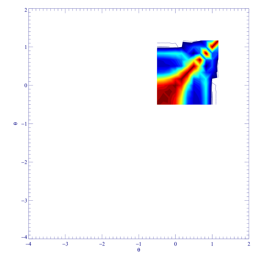
Figure 29: Correlation matrix from Gaussian estimates for the $21\leq r^{*}\leq 22$ magnitude bin.

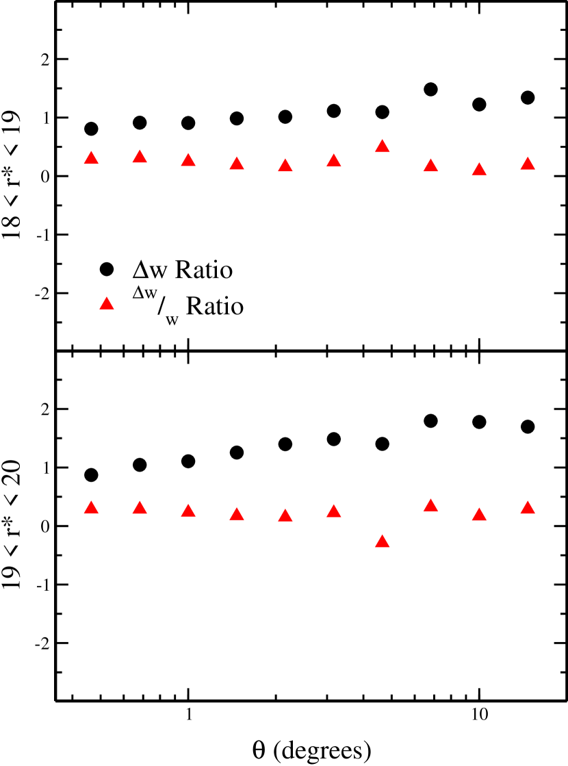
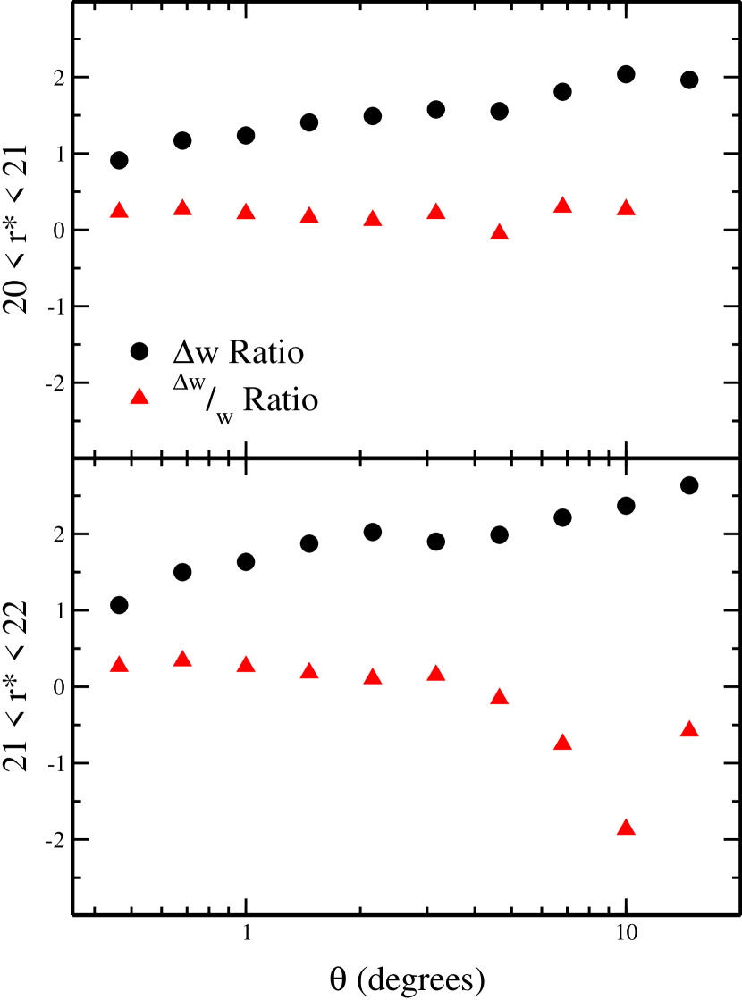
Figure 30: Ratios of $\Delta w$ and $\frac{\Delta w(\theta)}{w(\theta)}$ for the errors calculated using the Gaussian method compared to those found using the simulation technique for the four magnitude bins.

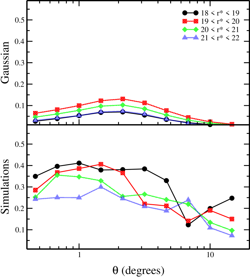
Figure 31: $R(\theta)$ calculations for the Gaussian correlation matrices and the corresponding elements of the simulation correlation matrices.

We can use the same tools developed in the previous sections to analyze the agreement between the simulation errors and the Gaussian errors. Figure 29 shows the correlation matrix for the Gaussian method in the $21\leq r^{*}\leq 22$ magnitude bin and Figure 30 shows ratios of $\Delta w(\theta)$ and $\frac{\Delta w(\theta)}{w(\theta)}$ comparing the Gaussian errors to the errors from the simulation. Likewise, in Figure 31, we give the calculation for $R(\theta)$ for the Gaussian errors along with the $R(\theta)$ for the same elements of the simulation correlation matrix. As with the previous analysis, the $\Delta w(\theta)$ ratios agree to within factors of 1-2, although the ratios of $\frac{\Delta w(\theta)}{w(\theta)}$ do demonstrate a clear difference in the large-angle behavior of $w(\theta)$ for the simulations and the data. It is clear, however, that the disparity is due to different values for $w(\theta)$ for the two data sets and not due to a large disagreement between the errors. For this reason (as well as the computational difficulty of applying the Gaussian method to the set of simulated catalogs), we will forego the Wishart test for the Gaussian errors.

13 Conclusions

The SDSS will ultimately make definitive measurements of the angular clustering of galaxies. To demonstrate the quality of the photometric data produced by the SDSS, we studied two nights of commissioning data that constitutes roughly a third of the Early Data Release. We presented a means to extract galaxy probabilities from the output parameters of the photometric data processing pipeline. With this in hand, we analyzed the effect of external factors (seeing variations, reddening extinction, stellar contamination and sky brightness) on that star/galaxy method. After implementing cuts due to seeing, and to a lesser extent reddening and bright stars, we find no evidence for external systematic effects polluting the measurement of the angular correlation function.

Having addressed external sources of error, we turned our attention to internal sources. We investigated the possibility of differential photometric response across the CCDs as well as the introduction of correlations due to different photometric calibrations between the two runs that made up our data area. We verified that the $w(\theta)$ measurements scaled according to Limber’s equation in a $\Lambda$CDM cosmology and we were able to simulate possible deblending errors, placing a lower limit on the angular extent of our clustering measurements. As with the external systematic error checks, we were able to effectively eliminate systematic errors after placing some constraints on the measurement.

Once the systematic errors were addressed for the broader category of angular measurements, we shifted our focus to the actual measurement of $w(\theta)$. Using two complementary estimators, we were able to devise a scheme for calculating $w(\theta)$ and its covariance using a reasonable amount of CPU time. We presented a prescription for addressing the integral constraint incurred due to a finite survey size and verified that the correction was much less than our measured $w(\theta)$. Three methods were discussed for calculating the covariance of $w(\theta)$: simulations, sub-samples and jackknife. The covariances from the simulations proved most reliable over the whole range of angular scales, but the jackknife errors would probably be adequate in the absence of simulations. Finally, we compared the covariances from the simulations to estimates of the covariance using a Gaussian assumption. The Gaussian covariances generally had smaller off-diagonal elements, but the diagonal elements agreed with the simulations to within a factor of 2.

Companion papers will present the results for the angular correlation function $w(\theta)$ (Connolly et al. 2001) and the angular power spectrum, $C_{l}$ (Tegmark et al. 2001). Using these measurements and estimates of the selection function, Dodelson et al. (2001) will extract the underlying 3D power spectrum and fit cosmological parameters. A parallel analysis of the data using a KL decomposition (Szalay et al. 2001) will provide another set of parameter constraints.

Though they constitute only a small fraction of the data, the initial results strongly suggest that the remaining $98\%$ of SDSS photometric data will provide a powerful and robust set from which to gain cosmological information.

14 Acknowledgements

The Sloan Digital Sky Survey (SDSS) is a joint project of The University of Chicago, Fermilab, the Institute for Advanced Study, the Japan Participation Group, The Johns Hopkins University, the Max-Planck-Institute for Astronomy (MPIA), the Max-Planck-Institute for Astrophysics (MPA), New Mexico State University, Princeton University, the United States Naval Observatory, and the University of Washington. Apache Point Observatory, site of the SDSS telescopes, is operated by the Astrophysical Research Consortium (ARC).

Funding for the project has been provided by the Alfred P. Sloan Foundation, the SDSS member institutions, the National Aeronautics and Space Administration, the National Science Foundation, the U.S. Department of Energy, the Japanese Monbukagakusho, and the Max Planck Society. The SDSS Web site is http://www.sdss.org/.

Support for this work was provided by the NSF through grant PHY-0079251 as well as by NASA through grant NAG 5-7092 and the DOE.

15 References

Bernstein, G.M. 1994, ApJ , 424, 569

Bouchet, F. R., Colombi, S., Hivon, E., & Juszkiewicz, R. 1995, A & A , 296, 575

Buchert, T., Melott, A.L., & Weiss, A. G. 1994, A & A , 288, 697

Collins, C.A., Nichol, R.C., & Lumsden, S.L. 1992, MNRAS , 154, 295

Connolly, A. et al., 2001, submitted to ApJ , (astro-ph/0107417)

Dodelson, S. et al., 2001, submitted to ApJ , (astro-ph/0107421)

Efstathiou, G. & Moody, S. J. 2000, astro-ph/0010478

J.H. Friedman, J.L. Bentley, & R.A. Finkel 1977, ACM Transactions on Mathematical Software, 3(3):209

Fukugita, M., Ichikawa, T., Gunn, J.E., Doi, M., Shimasaku, K., & Scheider, D.P., 1996, AJ, 111,1748

Fukugita, M., Yamashita, K., Takahara, F., Yoshii, Y., 1990, Ap. J. Let. , 361, L1

Gray, A. & Moore, A. W. 2001, Proceedings of Advances in Neural Information Processing Systems, 13

Gunn, J. E., & The SDSS Collaboration, 1998,AJ, 116, 3040

Hamilton, A.J.S. 1993, ApJ , 417, 19

Hui, L. & Gaztanaga, E. 1999, ApJ , 519, 622

Huterer, D., Knox, L., & Nichol, R. C. 2000, astro-ph/0011069

Ivezic, et al., 2001, in preparation

Kauffmann, G., Colberg, J.M., Diaferio, A. & White, S.D.M. 1999, MNRAS , 303, 188

Landy, S. D, & Szalay, A. S. 1993, ApJ , 412, 64

Lin, H., Yee, H. K. C., Carlberg, R. G., Morris, S. L., Sawicki, M., Patton, D. R., Wirth, G., & Shepherd, C. W., 1999, ApJ , 518, 533

Lupton, et al., 2001, in preparation

Maddox, S. J., Efstathiou, G., Sutherland, W. J., & Loveday, L. 1990, MNRAS , 242, 43P

Maddox, S.J. Maddox, Efstathiou, G., Sutherland, W.J., 1996, MNRAS , 283, 1227

Moutarde, F., Alimi, J.-M., Bouchet, F.R., Pellat, R., & Ramani, A. 1991, ApJ , 382, 377

Navarro, J.F., Frenk, C.S. & White, S.D.M. 1997, ApJ , 490, 493

Peacock, J. A. & Dodds, S. J. 1994, MNRAS , 267, 1020

Peebles, P.J.E. 1980, The Large Scale Structure of the Universe (Princeton University Press)

Petrosian, V., 1976, ApJ , 209, L1

Schlegel, D.J., Finkbeinder, D. P., & Davis, M. 1998, ApJ , 500, 525

Scoccimarro, R. 2000, ApJ , 544, 597

Scoccimarro, R., Sheth, R.K., Hui, L. & Jain, B. 2001, ApJ , 546, 20

Scoccimarro, R. & Sheth, R.K. 2001, astro-ph/0106120

Sheth, R.K. & Lemson, G. 1999, MNRAS , 305, 946

Sheth, R.K. & Diaferio, A. 2001, MNRAS , 322, 901

Szalay, A.S. et al., 2001, submitted to ApJ , (astro-ph/0107419)

Szapudi, S., Colombi, S. & Bernardeau, F. 1999, MNRAS , 310, 428

Szapudi, S., Szalay, A. S. 1998, Ap. J. Let. , 494, L41

Tegmark, M. et al., 2001, submitted to ApJ , (astro-ph/0107418)

Tegmark, M., Hamilton, A. J. S., Strauss, M. A., Vogeley, M. S., & Szalay, A. S. 1998, ApJ , 499, 555

Wichern, D.W. & Johnson, R.A., 2002, Applied Multivariate Statistical Analysis, ${\rm 5^{th}}$ Edition, (Prentice Hall)

Yasuda, N. et al. 2001, AJ, 122, 1104

York, D. G., & The SDSS Collaboration 2000, AJ120, 157

Zehavi, I. et al. 2002, ApJ , 571, 172

Figure 2: Concentration histogram for a section of run 756 for objects with $20.0\leq r^{*}\leq 20.5$.

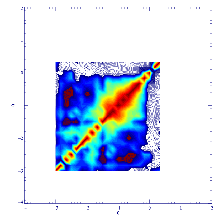
Figure 23: Same as Figure 22, but for the sub-sample method.

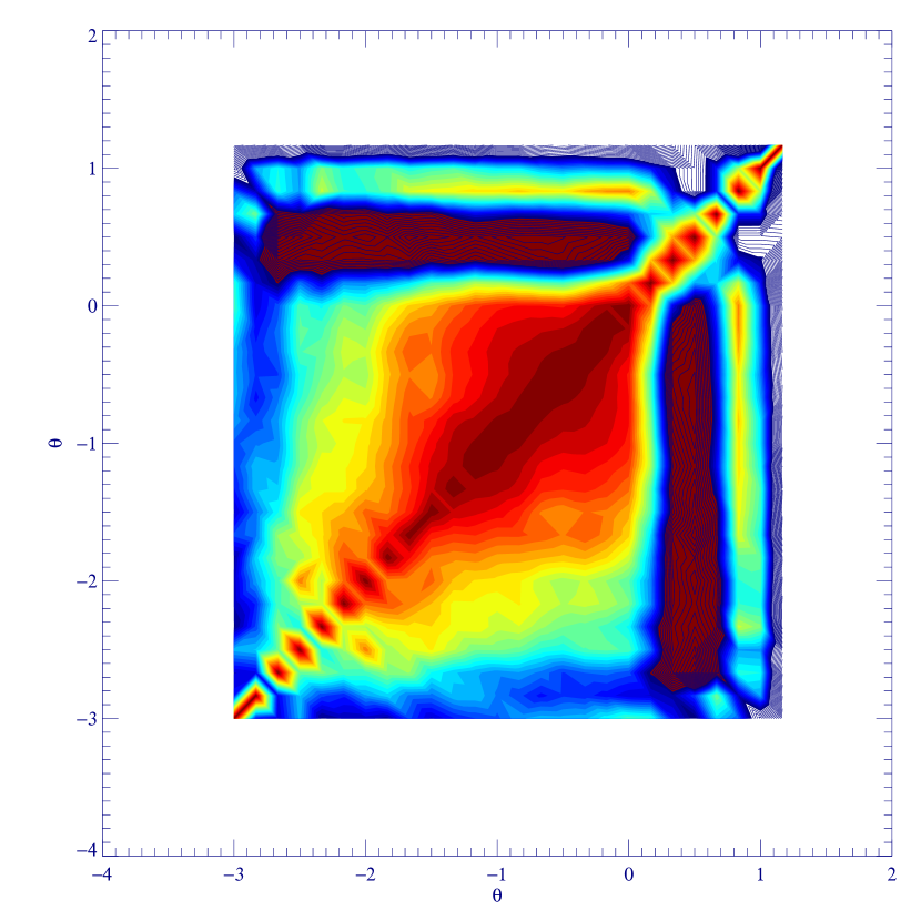
Figure 24: Same as Figure 22, but for the jackknife method.

Table 1: $\chi^{2}$ Values

Magnitude	Data $\chi_{J}^{2}/k$	Data $\chi_{S}^{2}/k$	Simulation $\chi_{J}^{2}/k$	Simulation $\chi_{S}^{2}/k$
$18\leq r^{*}\leq 19$	0.51	1.4	1.9	1.6
$19\leq r^{*}\leq 20$	0.46	0.21	2.2	1.8
$20\leq r^{*}\leq 21$	0.87	0.3	2.2	1.9
$21\leq r^{*}\leq 22$	0.57	0.43	2.2	2.0

Note. — The first two columns use the data-based jack-knife and sub-sample covariance matrices, respectively, to calculate $W(C_{S|J}|C_{M})$ using Equation 34. The third and fourth columns use covariance matrices calculated by applying the jackknife and sub-sample methods to the simulated data to calculate $W(C_{S|J}|C_{M})$.