PHOTOIONIZATION MODELS FOR BALQSO PG 0946+301

Abstract

This is a companion paper to the manuscript entitled: “HST STIS Observations Of PG 0946+301: The Highest Quality UV Spectrum Of A BALQSO” (Arav et al. 2001; accepted for publication in the ApJ). Here we present photoionization-modeling results for all the ionic column density constraints found in these data, most of which we were unable to include in the printed version of the paper.

1 DESCRIPTION

In the following pages we present photoionization-modeling results for all the ionic column densities constraints found in the HST/STIS spectra of PG 0946+301. We use the $N_{\scriptscriptstyle H}$/$U$ plane presentation, applied to optically thin slabs, which is described in § 4 of the main paper. Two incident spectra are used for the CLOUDY models, the standard Mathews–Ferland AGN spectrum and a modified $\alpha$=–2 power-law spectrum which is more consistent with the observed far UV spectral shape of the PG 0946+301 spectrum. Both spectra are shown in figure 1. Figures 2–4 show the results for the modified $\alpha$=–2 power-law spectrum. In figure 2 we include only the hydrogen and helium results, for helium we have an upper limit which therefore excludes the parameter area above the curve. Figure 3 shows results for the available ionic constraints from 8 “metals.” Each curve is labeled by its corresponding ion and the number beneath the label is the $\log(N_{ion})$ constraint. An * following the $\log(N_{ion})$ denotes an upper limit (excluding the parameter area above the curve), otherwise the constraint is a lower limit (excluding the parameter area below the curve). The small box at the center of the plots identifies the area in parameter space which is fully consistent with 21 ionic constraints, marginally inconsistent with 3 and is strongly inconsistent with 2 (see § 4 for details). Figure 4 is identical to figure 7 in the main paper.

Figures 5–8 are similar to figures 2–4, using the Mathews–Ferland AGN spectrum. To ease the comparison between results from the two incident continua, we left the parameter space box at the same location as for the power-law spectrum.

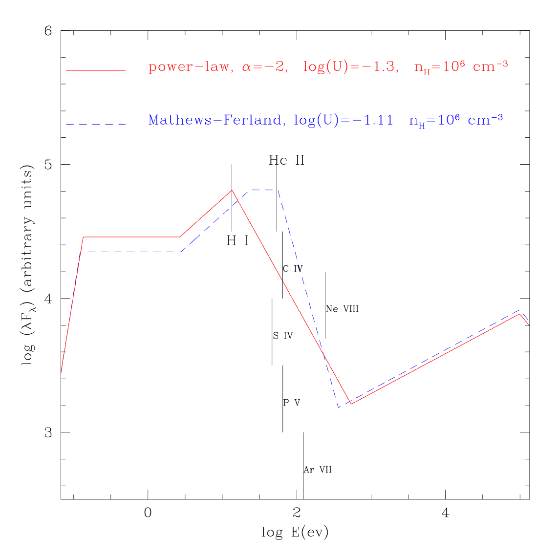
Figure 1: Comparison between Mathews–Ferland and a modified $\alpha=-2$ power-law spectrum, which is consistent with the observed far UV spectral-shape of the PG 0946+301 spectrum. Ionization potentials for several important ions are marked by short vertical lines.

Figure 2: The all-important hydrogen constraints and their origin for the modified $\alpha=-2$ power-law spectrum. Also shown is the He i constraint.

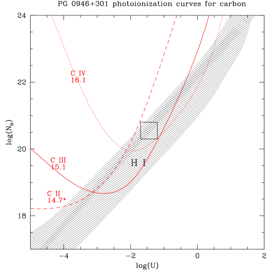
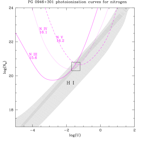
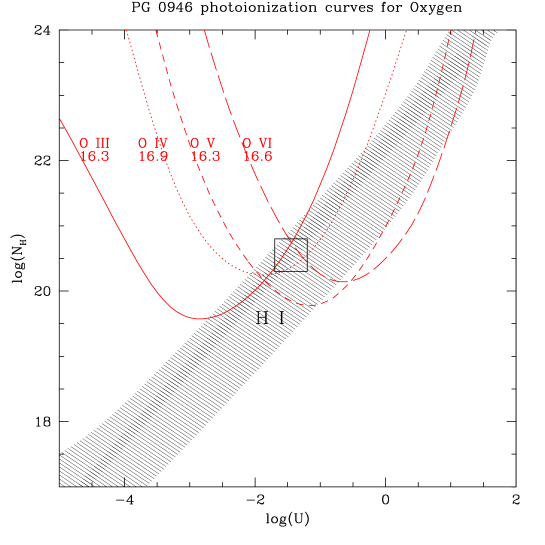
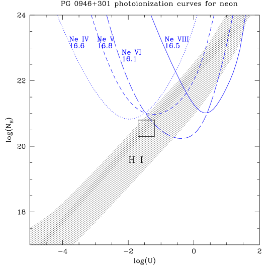
Figure 3: Metal-ion constraints for the modified $\alpha=-2$ power-law spectrum, an * following the $\log(N_{ion})$ value denotes an upper limit (excluding the parameter area above the curve), otherwise the constraint is a lower limit (excluding the parameter area below the curve).

Fig. 3 continued

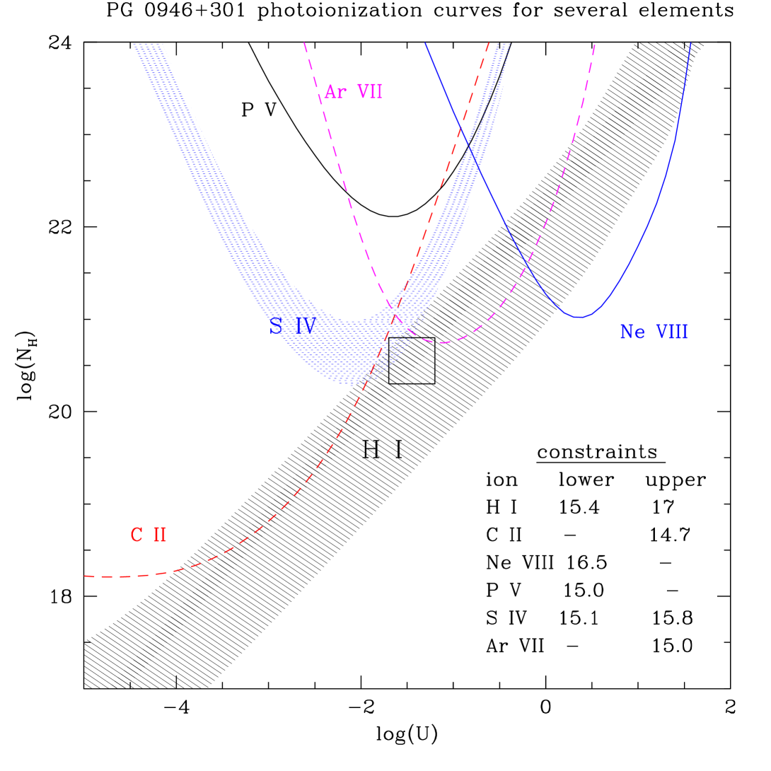
Figure 4: Some of the more important ionization constraints from several elements (identical to Fig. 7 in the main paper).

Figure 5: The all-important hydrogen constraints and their origin for the Mathews–Ferland spectrum. Also shown is the He i constraint.

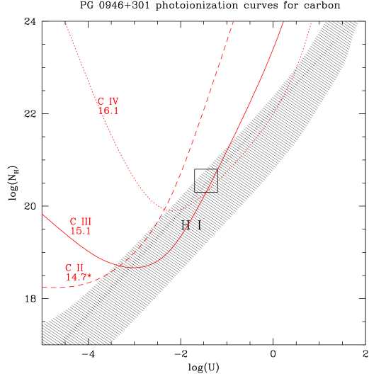
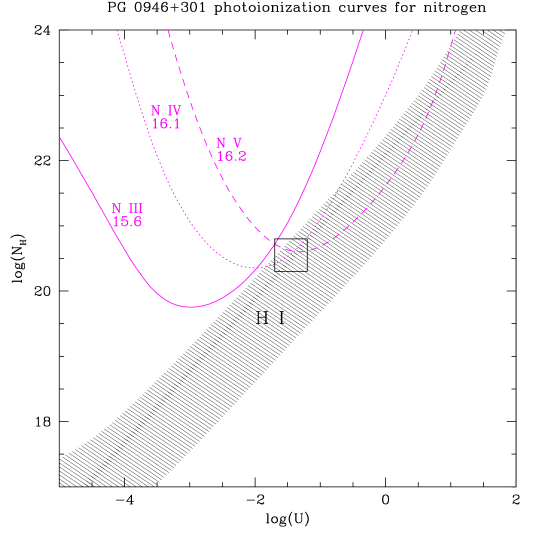
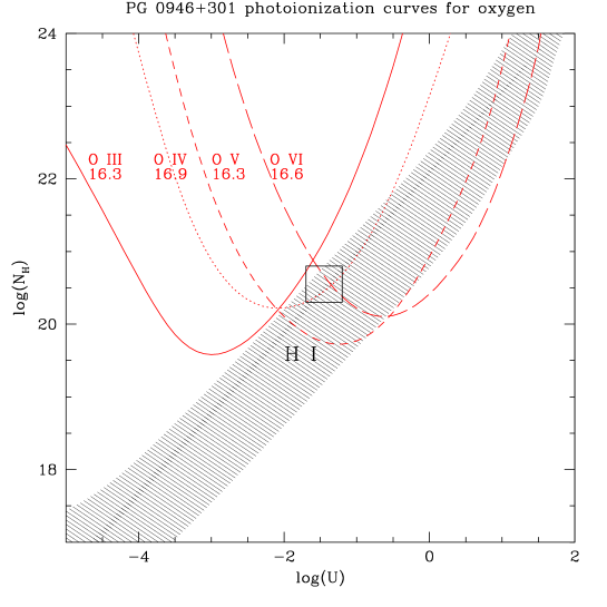
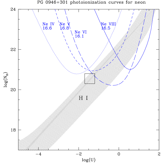
Figure 6: Metal-ion constraints for the Mathews–Ferland spectrum, an * following the $\log(N_{ion})$ value denotes an upper limit (excluding the parameter area above the curve), otherwise the constraint is a lower limit (excluding the parameter area below the curve).

Fig. 6 continued

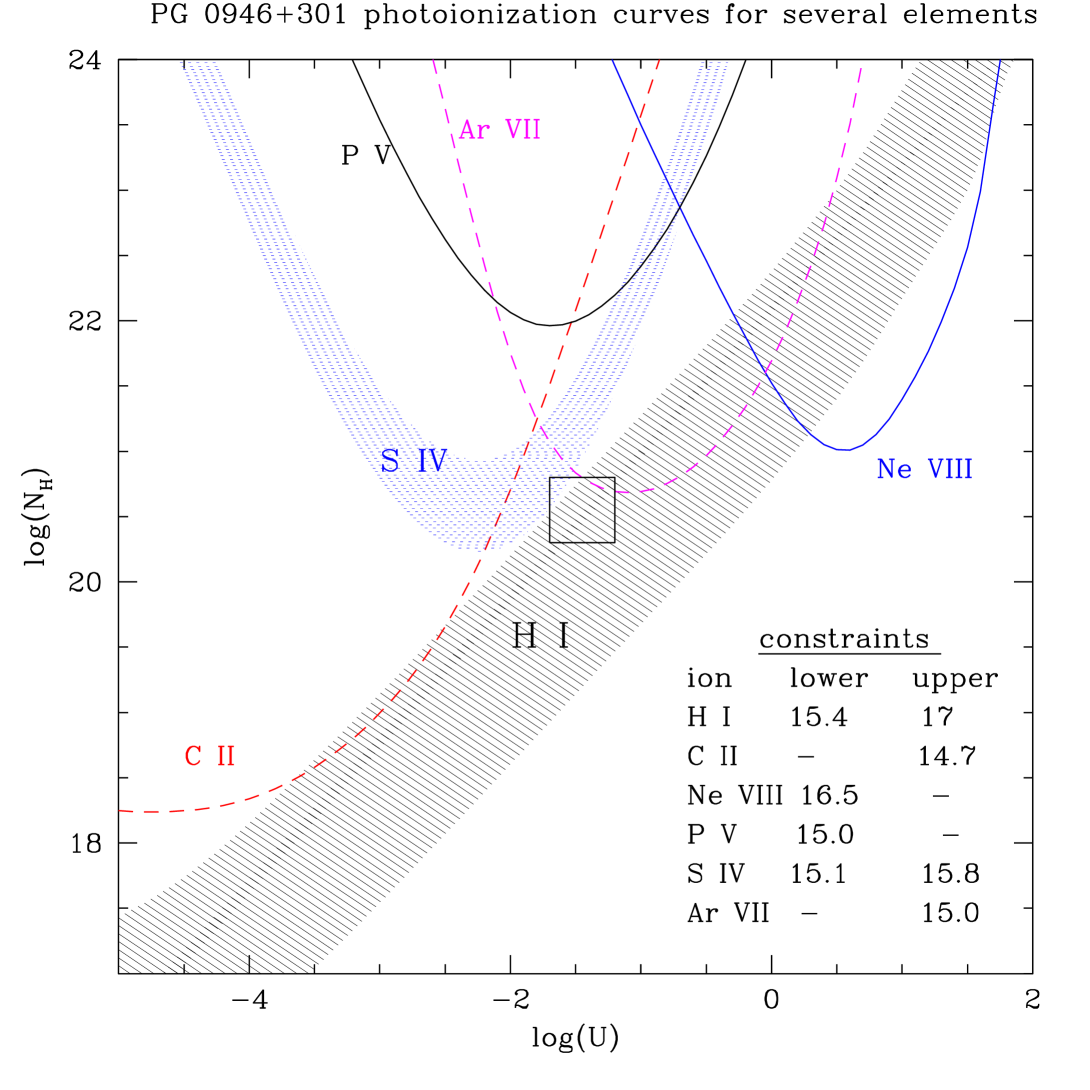
Figure 7: Some of the more important ionization constraints from several elements for the Mathews–Ferland spectrum.