HST STIS OBSERVATIONS OF PG 0946+301:
THE HIGHEST QUALITY UV SPECTRUM OF A BALQSO

ABSTRACT

We describe deep (40 orbits) HST/STIS observations of the BALQSO PG 0946+301 and make them available to the community. These observations are the major part of a multi-wavelength campaign on this object aimed at determining the ionization equilibrium and abundances (IEA) in broad absorption line (BAL) QSOs. We present simple template fits to the entire data set, which yield firm identifications for more than two dozen BALs from 18 ions and give lower limits for the ionic column densities. We find that the outflow’s metalicity is consistent with being solar, while the abundance ratio of phosphorus to other metals is at least ten times solar. These findings are based on diagnostics that are not sensitive to saturation and partial covering effects in the BALs, which considerably weakened previous claims for enhanced metalicity. Ample evidence for these effects is seen in the spectrum. We also discuss several options for extracting tighter IEA constraints in future analyses, and present the significant temporal changes which are detected between these spectra and those taken by the HST/FOS in 1992.

Subject headings: quasars: absorption lines — quasars: individual (PG 0946+301)

1 INTRODUCTION

Broad Absorption Line (BAL) QSOs are a spectacular manifestation of AGN outflows. BALs are associated with prominent resonance lines such as C iv $\lambda$1549, Si iv $\lambda$1397, N v $\lambda$1240, and Ly$\alpha$ $\lambda$1215. They appear in about 10% of all quasars (Foltz et al. 1990) with typical velocity widths of $\sim 10,000$ km s^-1 (Weymann, Turnshek, & Christiansen 1985; Turnshek 1988) and terminal velocities of up to 50,000 km s^-1. The small percentage of BALQSOs among quasars is generally interpreted as an orientation effect, and it is probable that the majority of quasars and other types of AGN harbor intrinsic outflows (Weymann et al. 1991).

Establishing the ionization equilibrium and abundances (IEA) of the BAL material is a fundamental issue in quasar studies (Weymann, Turnshek, & Christiansen 1985; Wampler, Chugai & Petitjean 1995; Hamann 1996; Korista et al. 1996; Arav et al. 2001; de Kool et al. 2001). Furthermore, determining the IEA is crucial for understanding the dynamics of the flows, especially radiative acceleration scenarios that are strongly coupled to the ionization equilibrium (Arav, Li & Begelman 1994; de Kool & Begelman 1995; Murray et al 1995; Arav 1996; Proga, Stone & Kallman 2000). Finally, the mass flux and kinetic luminosity associated with the flow cannot be constrained without a reliable IEA determination.

Careful spectroscopic analysis has made it apparent that the BALs are often saturated while not black (Arav 1997; Telfer et al. 1998; Churchill et al. 1999; Arav et al. 1999b; de Kool et al. 2001). Support for this picture comes from spectropolarimetry studies (Cohen et al. 1995; Ogle et al. 1999; Brotherton et al. 2001). As a result, BAL ionic column densities ($N_{ion}$) determined in the traditional way (from equivalent width or direct conversion of the residual intensity into optical depth) can only serve as lower limits to the real column densities. Since BAL column densities are the foundation of any attempt to determine the IEA in the outflows, it became clear that more sophisticated analyses are essential for any progress in understanding the BAL phenomenon. To derive real $N_{ion}$ we have to account for saturation and partial covering factor in the BALs. In the UV, this approach is currently feasible only for exceptionally bright BALQSOs and still requires long integration times. After studying the available BALQSO data in the HST archive and hundreds of ground based spectra, we concluded that PG 0946+301 is the best candidate for such analysis. It has a substantially higher flux between 1200–2500 Å (observed frame) than any other BALQSO that is suitable for IEA studies. Thus, we can obtain very high-quality data for a wide rest frame spectral region (500 – 1700 Å), and the object suffers only minor contamination by Ly$\alpha$ forest lines due to its low redshift ($z=1.223$). Finally, the BALs of PG 0946+301 are typical for a high-ionization BALQSO. For example, the balnicity index of the C iv trough is 6300 km s^-1, compared with 5000 km s^-1 for the BALQSO sample of Weymann et al. (1991).

It is for these reasons that many QSO researchers joined together to study PG 0946+301 with deep, high-quality multi-wavelength observations. The components of the campaign were: HST UV spectroscopy (described here), ASCA X-ray observations (Mathur et al. 2000), FUSE UV spectroscopy (25 ksec data currently under analysis by the FUSE PI team), high-resolution optical spectroscopy and optical spectropolarimetry (some data already taken, other observations planned).

In this paper we describe the Space Telescope Imaging Spectrograph (STIS) observations, present simple template fits for the BALs and discuss our preliminary IEA findings. We make the data (including some ground based spectra) available to the community in order to facilitate future analyses of this unique data set. In § 2 we elaborate on the data acquisition, reduction and wavelength calibration of the observations, and outline the temporal changes in the BALs detected by comparing the 1992 HST/FOS spectrum to the STIS data. We defer most of the temporal analysis to a future paper. In § 3 we describe our template fitting analysis for the entire spectrum, including the derivation of optical depth templates, line identifications and unidentified absorption features, and also discuss possible improvements over the template fitting technique. In § 4 we describe the IEA constraints obtained from the current analysis and discuss the over-abundance of phosphorus. In § 5 we summarize our results.

Figure 1: Composite STIS spectrum of PG 0946+301. Flux is measured in the observed frame. The bottom labels identify the ions responsible for the major absorption features. Some of the broad emission lines are marked above the spectrum. The dotted line designates zero intensity and the solid line above it is the noise spectrum.

2 OBSERVATIONS

2.1 Data Acquisition and Reduction

We observed PG 0946$+$301 with the Space Telescope Imaging Spectrograph (STIS) on the Hubble Space Telescope (HST) over a three-month period in early 2000. All of the spectra were obtained through a 52^′′ x 0${}^{\prime\prime}\!.$2 slit to maximize throughput without a significant loss in spectral resolution. We used the MAMA detectors and G140L and G230L gratings to obtain full UV coverage at a resolution of 1.2 Å and 3.2 Å, respectively. We also used the CCD detectors and the G430M grating to obtain limited coverage in adjacent optical regions at a resolution of 0.56 Å. The details of the observations are given in Table 1.

Each G140L or G230L entry in Table 1 represents a five-orbit visit, since STIS MAMA observations are limited to five consecutive orbits due to constraints imposed by the South Atlantic Anomaly. To maximize the signal-to-noise of the spectra, we obtained exposures at five different locations separated by 0${}^{\prime\prime}\!.$3 along the slit (one location per orbit). We used this strategy to place the spectra at slightly different positions on the detector, to avoid possible fixed pattern noise not removed by the flat-fielding of the spectra (Kaiser et al. 1998). For the G430M observations, we obtained two spectra per orbit (at the standard slit locations) to accumulate enough images to allow for accurate cosmic-ray rejection.

We reduced the spectra using the IDL software developed at NASA’s Goddard Space Flight Center for the STIS Instrument Definition Team (Lindler 1999). The individual spectra from each orbit were independently calibrated in wavelength and flux, and resampled to a linear wavelength scale (retaining the same average dispersion). Careful examination of the spectra from each orbit reveals no discernible change in flux over time or as a function of position on the detectors. We therefore averaged the spectra (weighted by exposure time) to obtain final versions of the G140L, G230L, and two G430M spectra. These were then combined into a single spectrum using Galactic absorption lines for a final wavelength calibration. The resultant spectrum and its noise are shown in Figure 1.

Table 1: HST/STIS Observations of PG0946$+$031

Grating	Range	Exposure	Date
	(Å)	(sec)	(UT)
G140L	1140 – 1715	12,960	2000 February 26
G140L	1140 – 1715	12,960	2000 March 28
G140L	1140 – 1715	12,960	2000 March 30
G140L	1140 – 1715	12,960	2000 April 4
G140L	1140 – 1715	12,960	2000 May 11
G430M	3022 – 3306	5,274	2000 April 12
G430M	3163 – 3447	7,250	2000 April 12
G230L	1640 – 3148	12,960	2000 April 23
G230L	1640 – 3148	12,960	2000 May 2

2.2 Comparison of the FOS and STIS Data

Figure 2: The C iv spectral region in PG 0946+301 at two different epochs. Histogram: STIS data from March 2000; dotted line: FOS and Lick data from 1992. The two settings of the G430M STIS grating are shown (rebinned by 10 pixels), these overlap between 3165 – 3300 Å. In the main trough (3260 – 3400 Å) there is a significant deepening of the absorption in the 2000 data and a new high velocity trough is seen between 3130 – 3250 Å. We note that the differences are very significant compared to the noise level and that the STIS data are in remarkable agreement with Lick data from the same epoch (not shown here).

PG 0946+301 was observed by the HST Faint Object Spectrograph (FOS) in 1992. These data are still among the highest quality UV spectra of BALQSOs (complete analysis of these observations is found in Arav et al. 1999a, hereafter FOS99). Combined with the much higher S/N STIS data, we possess a unique data set for studying the temporal changes in the many BALs observed in the UV. In addition, we have five epochs of the C iv trough obtained from ground based telescopes. We defer a full analysis of the observed temporal changes to a separate paper. Here we briefly describe the main changes and concentrate on the ones that affect our model fits most.

In Figure 2 we show the C iv spectral region at two epochs separated by 8 years ($\sim$3.5 years in the rest frame of the object). The 1992 spectrum is a combination of the HST data from the FOS G270H grating ($\lambda<3250$ Å, with a four pixel rebinning), and Lick data ($\lambda>3250$ Å). The 2000 observations consist of two setting of the STIS G430L grating rebinned by 10 pixels (see Table 1 for exact dates and exposure times). Our Lick 2000 data (not shown here) are in remarkable agreement with the STIS G430L data. Inspection of Figure 2 reveals several significant changes between the 1992 and 2000 spectra.

1. Significant deepening of the main trough has occured between 3260 – 3400 Å (observed frame). For comparison the S/N level at the deepest part of the trough is 6.5 for the Lick 1992 data and 7 for the binned STIS data.

2. A substantial decrease in flux is seen between 3280 – 3300 Å ($\sim$ 25%). A similar change is also easily identified in the N v and O vi BALs.

3. A new shallow high velocity trough is seen in the STIS data between 3130 – 3250 Å (–17,200 to –28,400 km s^-1), with a maximum depth of 20%. Several other high ionization BALs show this feature (most evident in N v and O vi). The high velocity trough is not present in low ionization species (Si iv, C iii, N iii…).

4. The Si iv absorption depth in the broad low velocity trough (–4000 to –7000 km s^-1) has increased significantly (not shown in the figure), and this can also be seen in other low-ionization species (e.g. O iii, N iii).

Both independent settings of the G430L grating show the new high velocity BAL as well as the decrease in flux that is seen between 3280 – 3300Å. We also note that while the Si iv BEL is 20% stronger in the STIS data, the C iv BEL has not changed appreciably (based on the Lick 2000 data).

3 TEMPLATE FITTING ANALYSIS

The simplest way of analyzing an absorption line spectrum containing many broad overlapping lines with a complex velocity structure is the template fitting approach (Korista et al. 1992; FOS99). This method uses the apparent optical depth (defined as $\tau=-ln(I_{r})$, where $I_{r}$ is the residual intensity seen in the trough, for more details see FOS99) profile of a given ionic transition as a template to fit all other transitions, where only a simple multiplicative scaling is allowed. The fitting process finds the optimum scaling values which minimize the difference between the data and a model spectrum based on using scaled versions of the template for all plausible transitions. We did this in two ways. First, we used standard $\chi^{2}$ statistics, i.e., minimized the square of the differences between the model and the data, weighted by the square of the Poisson error. However, because the S/N ratio is very high everywhere, the deviations between the model and the observations are almost entirely due to uncertainties regarding the effective continuum (defined below) and covering factor effects. Therefore, we also fit the spectrum using a constant error rather than the Poisson error at each wavelength point. In practice using a constant error or the statistical error changes the parameters derived from the fit by less than 0.1 dex so that the exact minimization method used is irrelevant.

The fitted scaling factors are translated to ionic column densities $(N_{ion})$ using standard techniques (see below). Two assumptions must hold in order that the fitted $N_{ion}$ be good approximations for the real ones. First, the absorbing material covers the emission source completely and uniformly, and scattered-photons do not contribute appreciably to the residual intensity in the trough (see discussions in Korista et al. 1992; Arav 1997). Second, the ionization equilibrium does not vary as a function of velocity. As we will show, the first assumption is not a good approximation for the BALs in PG 0946+301. In this case we must treat the fitted $N_{ion}$ as lower limits for the real ones (FOS99, Arav et al. 1999b, de Kool et al. 2001).

3.1 Methodology

Using the assumptions described above, the optical depth at a given wavelength $\lambda$ due to a transition between levels $l$ and $u$ of species $n$ can be expressed as

$$\tau_{nlu}(\lambda)=\frac{\pi{e}^{2}}{m_{e}c}\lambda_{lu}f_{lu}\frac{X_{nl}}{X_{0}}\frac{dN_{0}}{dv}\biggr{|}_{v=v(\lambda_{lu}\rightarrow\lambda)}$$ (1)

Here $\lambda_{{lu}}$ and $f_{lu}$ are the rest wavelength and oscillator strength of the transition, $\frac{X_{nl}}{X_{0}}$ the density ratio between ions of species $n$ in energy state $l$ and some reference species for which the distribution of column density over velocity $\frac{dN_{0}}{dv}$ is known, and ${v(\lambda_{lu}\rightarrow\lambda})$ is the velocity that shifts a line with rest wavelength $\lambda_{lu}$ to the wavelength $\lambda$. The distribution of column density over velocity $\frac{dN_{0}}{dv}$ is usually derived from the optical depth in a transition corresponding to a line that is not blended with other lines:

$$\frac{dN_{0}}{dv}=\frac{{m_{e}c}}{\pi\/{e}^{2}}\frac{1}{\lambda_{0}f_{0}}\tau_{\scriptscriptstyle 0}(v)$$ (2)

It can be derived directly if the transition is a singlet (e.g. de Kool et al. 2001), or by a deconvolution if the transition is a multiplet (e.g., FOS99). The line profile $\tau_{\scriptscriptstyle 0}(v)$ of the reference transition thus serves as a template for all other absorption lines.

Once the template is known, a model of the total optical depth as a function of wavelength is constructed based on a first guess of the ratio of the column density of each species relative to that of the reference species, $\frac{X_{nl}}{X_{0}}$:

$$\tau(\lambda)=\sum_{n}\sum_{l}\sum_{u>l}\tau_{nlu}(\lambda)$$ (3)

Using the derived $\tau(\lambda)$ and a model for the unabsorbed continuum, a model spectrum is computed that can be compared with the observed spectrum. Using an iterative procedure, the values of $\frac{X_{nl}}{X_{0}}$ are then adjusted until the $\chi^{2}$ is minimized. The value of $\frac{X_{nl}}{X_{0}}$ of the best fit yields the ratio of the column density of ion $n$ in energy state $l$ to the column density of the reference species. In the current analysis we assume that the ground-term level populations of the ions we consider are in LTE, at a temperature much higher than the level energy, so that the relative population of each energy level in the ground-term is proportional to its statistical weight.

3.2 The Velocity Templates

As in our previous study of PG 0946+301 we used templates derived from two reference transitions. C iv $\lambda$1548.20 is used for lines from high ionization species, and Si iv $\lambda$1393.76 for lines from low ionization species, both lines are the blue component of their respective doublets. In Figure 3 we present the C iv and Si iv optical depth as a function of velocity derived from the STIS spectrum of PG 0946+301. The template for C iv was obtained with a regularization method similar to that described in FOS99. Because of the much higher resolution in the observed C iv line, the regularization used in FOS99 which suppressed fluctuations in neighboring points did not give satisfactory results. Instead, we used an alternative form of the regularization matrix H, in the notation of FOS99: $h_{i,i}=2$, $h_{i,i+s}=-1$, $h_{i,i-s}=-1$ and all other elements of H equal to zero. This form suppresses oscillations on the scale of the doublet separation but does not smooth the derived profile over neighboring points. The value of the regularization parameter used was 0.1. We derived the Si iv template without regularization, since oscillations on the scale of the doublet are not apparent in the plain deconvolution result.

Figure 3: The apparent optical depth as a function of velocity for the blue components of the C iv $\lambda$1549, (thin line) and Si iv $\lambda$1397 (thick line) resonance doublets.

The transition between data from the G230L grating and the G430M grating, and the accompanying change in spectral resolution, occurs in the middle of the Si iv line. This accounts for the smooth appearance of the high velocity part of the Si iv template. There is no evidence of the new high velocity trough in the Si iv absorption line. The Si iv template was corrected for the presence of intervening C iv absorption at 1330 Å in the QSO restframe by removing this line from the spectrum before the deconvolution. We note that some of the absorption in the range –11,000 to –13,000 km s^-1 may be due to C iv from another intervening system that can be identified from its Ly$\alpha$ absorption (component 9 in Table 2 in FOS99). There is some evidence for this being the case from the fact that the Si iv template over-predicts absorption in other low ionization species (eg, O iii, S iv) at these velocities.

3.3 The Effective Continuum

In order to make measurements or fit the observed BALs we must use a model for the unabsorbed emission (continuum plus BELs, hereafter “the effective continuum”) of the quasar. At wavelengths longer than $\sim$ 1000 Å, the spectrum of PG 0946+301 is very close to the non-BALQSO composite of Weymann et al. (1991), which we therefore used as our long wavelength effective continuum with only small modifications to some emission line strengths (as in FOS99). Shortwards of 830 Å we found only two narrow regions (624 – 631 Å and 567 – 571 Å) free from BAL features. This complicates the task of determining the effective continuum based on the data at hand. Unfortunately, very little is known observationally about intrinsic QSO spectra in the range 500 – 900 Å. The QSO composite spectrum of Zheng et al. (1998) does cover these wavelengths, but very few QSOs contribute to the composite in this wavelength range. Furthermore, the signal to noise ratio is so low that the use of this composite as a continuum would introduce too much noise to the analysis.

With these uncertainties in mind, we used a similar approach to the one we employed in the analysis of the HST FOS data. Three effective continua are employed (shown in Fig. 4). The first is a fixed continuum which is very similar to the fixed continuum in FOS99 (for details see § 5.2 of FOS99). We lowered the flat continuum shortwards of 900 Å by 5% and added two BEL features, one for O v $\lambda$630 and one for Ne v $\lambda$571. Both BELs are required by features evident in the STIS data (the quality of the FOS G160L data was too low to justify the addition of these BELs). Emission features of roughly the same shape and wavelengths are also seen in a smoothed version of the quasar composite spectrum produced by Zheng et al. (1998).

Figure 4: The three effective continua plotted on top of the data. Longward of 1020 Å they are indistinguishable from the one shown in Figure 5.

The second and third effective continua are different from the fixed continuum for wavelengths below 1060 Å. In this range, the underlying continuum flux $F_{c}$ was assumed to have the functional form

$$F_{c}=F_{0}+F_{1}\bigl{(}{{\lambda}\over{1060}}\bigr{)}^{\beta}e^{-{{\lambda_{cut}}\over{\lambda}}}$$ (4)

where $F_{0}$, $\beta$, $\lambda_{cut}$ and $F_{1}$ are free parameters with the constraint that the continuum matches the long wavelength one at 1060 Å. The values of the continuum parameters were determined by optimizing them simultaneously with the column densities of all species ($\frac{X_{nl}}{X_{0}}$) during the template fitting process. Since the continuum parameters were allowed to vary in the fitting process, we refer to the resulting continuum as a floating continuum. The difference between the two floating continua is that one is derived from a template fit that only includes resonance lines as opacity sources, whereas the other also allows for a Lyman edge opacity (as a free parameter). The equivalent widths of the model BELs were fixed during the fitting process. Finally, most of the known intervening absorption line systems were modeled with single Gaussians with fixed equivalent widths to minimize possible confusion with BAL structures.

3.4 Results of the Template Fits

The column densities resulting from the template fits are summarized in Table 3, and the fit itself (for the fixed continuum) is illustrated in Figure 5. Before discussing these results, we re-emphasize that column densities obtained from template fitting are in reality only lower limits because of partial covering effects. For some species we will also quote an upper limit on the column density. Such an upper limit can be derived if the species in question has at least one line with a much lower oscillator strength than the others, which is not detected. These upper limits are necessarily somewhat subjective since they depend on the shape of the effective continuum and possible blending with other lines. By stating that a line is not present we are in fact making a judgment as to what variations in the effective continuum would be reasonable. Therefore, the upper limits are derived in practice by manually changing the column density in the fit and comparing the model spectrum and the observed spectrum at the position of the weak line to see what column density could be present without conflicting with the observations.

Figure 5: Expanded view of a fit and the fixed effective continuum used in producing it. Most BAL features are identified by the absorbing ion. The short vertical lines mark intervening and Galactic absorption lines, which we superimpose on the effective continuum to account for non-BAL absorption features.

When inspecting Table 3, the first thing to note is that the derived column densities are insensitive to the exact choice of effective continuum. Even changes of 30% in the continuum level affect the column densities of the stronger lines by a similar amount (i.e., 0.1 dex in the table), while the effects of non-black saturation can increase the inferred column densities by a factor of three or more.

Here follows a summary of the individual results:

Hydrogen. The Ly$\alpha$ BAL is not very deep, leading to a low value for the column density ($\log(N_{H\,{\sc i}})=15.4$) derived from it. If the fit includes a Lyman edge due to the BAL outflow, the best fit Lyman edge corresponds to a column density of $\log(N_{H\,{\sc i}})=16.4$. The neutral hydrogen column density from the Lyman edge fit is still consistent with the upper limit derived from the absence of a clear signature for Ly$\beta$ and Ly$\gamma$ BAL, $\log(N_{H\,{\sc i}})<16.7$. In our ionization discussion (§ 4), we use a somewhat more conservative upper limit of $\log(N_{H\,{\sc i}})<17$ to allow for partial covering effects.

Helium. The upper limit quoted for He i is derived from the absence of a clear signature of the 584 Å resonance line. This is illustrated in Figure 6a.

Carbon. We do not detect any absorption feature associated with a C ii $\lambda 1335$ BAL. The upper limit for this line provides important ionization equilibrium constraints (see § 4). A C iii BAL is clearly detected and its deepest component is not severely blended with other BALs, so that the apparent column density is well defined. The maximum optical depth is very similar to that of other low ionization species (H i, N iii, Si iv), which strongly suggests that the low ionization BALs are essentially saturated and derive their shapes primarily from partial covering. The C iv BAL is one of the templates, so no new information can be derived from its template fits.

Nitrogen. N iii gives rise to several lines in different parts of the spectrum. The value for the N iii column density is driven mainly by the strongest lines around 685 Å, the other ones (991 Å and 764 Å) being both weaker and blended with stronger lines from other species. The column density for N iv is not very well determined since its BAL is a part of the large blended trough near 750 Å. The N v BAL is very deep, even though it falls under the Ly$\alpha$ emission line. This contrasts with the saturation effects in the low ionization species mentioned above, which set in at a much higher flux level and imply a low covering factor. The higher ionization BALs appear to cover a significantly larger part of the source than the low ionization BALs, including most of the Ly$\alpha$ BEL region.. This suggests a physical picture where at a given velocity interval there is lower density extended material, surrounding denser lower ionization material with smaller geometrical extension. (see FOS99 for a full discussion). The new shallow high velocity component is deeper in N v than expected based on scaling the C iv template, as illustrated by the fact that the flux in the fitted model significantly exceeds the observed flux at the wavelengths where this absorption occurs. Note that this is not likely to be a result of the uncertainty in the continuum level since a comparison between the current STIS observation and the 1992 FOS observation clearly shows the emergence of the new absorption component. The fact that the high velocity component is deeper in N v than in C iv suggests that it is highly ionized, which is supported by the strength of this component in O vi and S vi.

Oxygen. Oxygen is a unique element in this analysis since we have relatively unblended BALs for four consecutive ionization stages. O iii has two multiplets at 703 Å and 835 Å. The O iii BALs are reasonably well fit by the model. The maximum optical depth in O iii is higher than in the other low ionization species, which is consistent with the trend that ions with higher ionization potential (IP) tend to have a larger covering factor (The O iii IP is almost midway between the Si iv and C iv IPs). Unfortunately, there are no O iii lines that allow us to determine an upper limit for the column density. O iv has three groups of lines, and the fit is mainly driven by the one with the lowest oscillator strength around 609 Å. The other two BALs (554 Å and 789 Å) are part of the large troughs around 550 Å and 750 Å. If the 609 Å BAL is well fit, the other two BALS are predicted to be deeper than observed, giving rise to the very large $\tau_{max}$. Because this occurs close to the bottom of the trough, the difference between model and fit does not contribute as much to the overall $\chi^{2}$. Again, this demonstrates the effects of partial covering. The O v BAL is interesting in that it clearly demonstrates how complex the real BAL formation is compared to our simple model. O v $\lambda 630$ is a singlet and the main part of the absorption (from –4000 km s^-1 to –11,000 km s^-1) is not blended with any other BALs. If our assumptions were correct, we would expect the shape of the O v BAL to correspond well to the C iv velocity template. In reality, however the shape is quite different, with the main velocity component in the template at –10,000 km s^-1 being less deep than the broad component between –4000 km s^-1  and –9000 km s^-1. A possible explanation for this behavior is that in this part of the spectrum the source size is varying rapidly as a function of wavelength, perhaps because of the presence of partially uncovered emission lines. We consider it more likely that the problem lies with continuum/source size problems around 600 Å than with the template, since many other high ionization lines, including O vi, were fit very well with the C iv template. O vi also clearly shows the new shallow high velocity component.

Neon. Absorption lines from several ionization stages of neon are expected to occur in the spectrum of PG 0946+301, and the template fitting procedure finds very large column densities for all of them. However, the neon lines occur only within the two large blended troughs around 550 Å and 750 Å so that their apparent column densities are less reliable than those of most other ions. The exception is Ne v, its $\lambda$571 multiplet is the main source of opacity for the red edge of the 555 Å trough, and therefore its fitted value is quite reliable. The combination of the uncertainty in the real optical depth in the neon lines with their low oscillator strengths leads to large values for the column density that are not necessarily realistic. However, establishing the existence (or lack) of a Ne viii BAL is of particular importance in the context of ionization equilibrium constraints (see § 4). We therefore conducted a tailored fitting experiment to assess its existence. We fit only the 700 – 845 Å region and ignored the correlation with other lines from the same ion found in different parts of the spectrum. In this way we circumvent some of the non-physical restrictions associated with ignoring saturation and partial covering inherent in our fitting process, and obtain the best local fit possible. Figure 6b shows the data, a fit including Ne viii and a fit excluding it. The large improvement caused by the inclusion of Ne viii is clearly seen in the 768 – 777 Å  753 – 757 Å and 730 – 740 Å regions. We conclude that the presence of an appreciable Ne viii BAL ($\log(N_{Ne\,{\sc viii}})\mathrel{\raise 1.29167pt\hbox{$>$}\mkern-14.0mu\lower 2.58334pt\hbox{$\sim$}}16.5$) in PG 0946+301 is highly probable.

Magnesium. In our analysis of the FOS data we discussed the probable identification of the Mg x $\lambda\lambda$ 609,625 BAL, which was based on fits to low-quality data obtained by the G160L grating. Our vastly superior quality STIS G140L data do not show any features that can be attributed to this BAL. The excellent fit for the 580 – 605 Å region shown in Figure 5 does not include any Mg x contribution. However, the strong presence of BALs from O iv and O v do not allow the determination of an interesting upper limit for this ion, the value we obtain for the upper limit is 1–3 $\times 10^{16}$ cm^-2.

Silicon. We do not detect any absorption feature associated with a Si ii $\lambda 1263$ BAL. The upper limit for this line supplies similar ionization equilibrium constraints to those available from C ii (see § 4). A possible Si iii $\lambda 1206$ BAL would be blended with the Ly$\alpha$ and N v BALs, so that very tight constraints are not possible. There is no evidence of the main component at –10,000 km s^-1 in the spectrum, leading to the upper limit in Table 3. Like C iv, Si iv is one of our template species, therefore no new information is obtained from the fit.

Phosphorus. As in previous investigations, we find good evidence for the presence of a P v BAL. In spite of its high ionization potential, the profile of the P v BAL fits much better with the Si iv template than with the C iv template. This would be consistent with a picture in which the BAL region contains a component with a very high column density and a small covering factor, which is responsible both for lines of lower ionization species and for lines from very low abundance species (see FOS99 for a full discussion). A possible P iv $\lambda 950$ BAL would occur in a highly blended region of the spectrum, so that only a relatively uninteresting upper limit can be derived.

Sulphur. S iii has a large number of lines that are predicted to form very broad BALs without sharp features. Because of this, identification of S iii features is not very secure, and S iii is only marginally detected in the spectrum, as is illustrated in Figure 6c. S iv is very clearly present, and the STIS spectrum resolves the uncertainties associated with the S iv lines in the FOS spectrum of PG 0946+301 (see FOS99). The depths of the strongest S iv lines is similar to that of the low-ionization template. S iv gives rise to several lines with a range of oscillator strengths. This allows a determination of an upper limit on the S iv column density of $\log N(S\,{\sc iv})<15.8$ (based on S iv $\lambda\lambda$809,815), which makes S iv the species with the most tightly constrained column density in our analysis. S v on the other hand is very poorly constrained, and the global template fits yield a negligible column density for it. The reason for this is that the S v line almost coincides with one of the stronger O iv lines at 790 Å. As mentioned above, the O iv fit is driven by a very weak line that already over-predicts O iv absorption at the position of the S v BAL, so that the S v column density is driven to zero. Since S v has only one line, this can occur without incurring penalties for a bad fit in another part of the spectrum. The value quoted in Table 2 is derived from a local fit (700 – 850 Å), which suffers less from the effects described above. S vi is the strongest and deepest sulphur BAL, in agreement with the hypothesis that higher ionization species have a larger covering factor, although the BAL definitely has a profile that is slightly different from that of the other high ionization BALs. The shallow high velocity component is evident in S vi, where it is deeper than that in C iv.

Argon. Resonance lines of Ar iv, Ar v, Ar vi and Ar vii occur in the wavelength range covered by the STIS spectrum of PG 0946+301. None of these lines are detected. For Ar iv, Ar v and Ar vi this leads to upper limits to their column density $\sim 2\times 10^{16}$ cm^-2 because these species have lines with fairly small oscillator strengths. These limits do not provide interesting constraints. The situation is different for Ar vii which has a strong singlet (oscillator strength of 1.24) at 586 Å. Figure 6d shows a fit which includes the Ar vii line at the level of $1.3\times 10^{15}$ cm^-2. However, the fit is unphysical since at the expected position of maximum Ar vii optical depth (567 Å) we find a much higher residual intensity than the fitted value. (We note that the adjacent narrow absorption feature seen in the data just longward of this position is due to Galactic Si ii $\lambda$1260). In all the well identified BALs the deepest predicted feature is fitted much better. In addition the Ar vii fit does a very poor job in reproducing most of the surrounding spectral features. Based on these arguments, $10^{15}$ cm^-2 is a conservative upper limit for the Ar vii column density.

Figure 6: Fit tests used to determine the existence of marginal, or heavily blended species (see text for discussion). The observed spectrum is shown as histograms, the thick and thin lines represent models with and without the ion considered, respectively.

Iron. The spectrum was searched for the presence of BALs from Fe iii and Fe iv. Fe iii has approximately 130 transitions in the wavelength range considered, and if present, would give rise to relatively broad blended BALs, similar to the case of S iii. The strongest lines occur around 860 Å, and the absence of any detectable features corresponding to these leads to $\log N(Fe\,{\sc iii})<15.3$. Fe iv has a resonance multiplet centered around 525 Å. Including Fe iv does improve the fit at the very shortest wavelengths, but there is no clear feature corresponding to it.

Unidentified absorption features. We found several absorption features in the STIS data for which we do not have good identification with either expected BALs, or with intervening and Galactic absorption lines. Most prominent are the features at (observed wavelength): 1526 Å ($\tau\sim$1), 1484 Å ($\tau\sim$0.3), 1463 Å ($\tau\sim$0.3), 1277 Å ($\tau\sim$1). We note that the feature at 1526 Å is too deep and broad to be fully explained by Galactic Si ii $\lambda$1526 line, since it should not be stronger than the observed Si ii $\lambda$1260 feature.

Table 2: Fitted Column densities

Ion	Lines	$f_{ul}$	Template	$N_{ion}$	$\tau_{max}$	$\lambda(\tau_{max})$	$N_{ion}$	$N_{ion}$
H i	1215.67	0.416	A	15.4	0.82	1215.67	-	-
Ly lim	911.76	-	A	-	-	-	-	16.4
He i	584.33	0.285	A	$<$15.5	-	-	-	-
C ii	1335	0.127	B	$<$14.7	-	-	-	-
C iii	977.02	0.767	B	15.1	0.82	977.02	15.2	15.2
C iv	1549	0.285	A	16.1	3.34	1549	-	-
N iii	991	0.122	B	15.6	0.84	686	15.6	15.6
	764	0.082
	686	0.402
N iv	764.15	0.616	A	16.1:	4.22	764.15	16.1:	16.0:
N v	1240	0.235	A	16.2	2.88	1240	-	-
O iii	834	0.107	B	16.3	1.31	834	16.3	16.2
	703	0.137
O iv	789	0.110	A	16.9	8.83	554	16.8	16.8
	609	0.067
	554	0.335
O v	629.73	0.515	A	16.2	3.30	629.73	16.2	16.2
O vi	1034	0.199	A	16.6	5.04	1034	16.6	16.6
Ne iv	543	0.233	A	16.6:	2.68	543	16.6:	16.6:
Ne v	571	0.092	A	16.8	1.68	571	16.8	16.6
Ne vi	561	0.090	A	16.8::	1.56	561	16.8::	16.8::
Ne viii	774	0.302	A	16.5:	2.36	774	16.5:	16.5:
Si ii	1263	1.18	B	$<$14.2	-	-	-	-
Si iii	1206.50	1.68	B	$<$14.3	-	-	-	-
Si iv	1397	0.784	B	15.1	0.86	1397	-	-
P iv	950.66	1.16	B	$<$15.0	-	-	-	-
P v	1121	0.701	B	15.0	0.36	1121	-	-
S iii	680	1.64	B	14.9::	0.41	680	14.6::	14.6::
S iv	814	0.103	B	15.3	1.06	660	15.2	15.1
	750	0.749
	660	1.17
S v	786.47	1.42	A	15.2	0.70	786.47	-	-
S vi	937	0.665	A	15.8	1.81	937	15.8	15.8
Ar vii	585.75	1.24	A	$<$15.1	-	-	-	-
Fe iii	861	0.131	B	$<$15.3	-	-	-	-

3.5 Beyond Template Fitting: Deriving and Constraining Real $N_{ion}$

As discussed in the introduction, a main goal for further analysis of the PG 0946+301 STIS data is to derive real $N_{ion}$ for the BALs or at least useful constraints beyond the simple template lower limits. While not attempting such a full analysis here, we outline several promising approaches as well as potential difficulties for doing so.

An obvious place to start is to examine the departure of the template fits from the data. In cases where we have BALs from two or more lines from the same ion, these departures often indicate non-black saturation and may be used to determine the covering factor of the absorber. Two good examples are the O iv lines $\lambda$609 and $\lambda$554 with an oscillator strength ratio of 1:5. Inspection of our fits clearly shows that the $\lambda$554 line is expected to be black if the $\lambda$609 is well fit. Since the $\lambda$554 trough is not black, we conclude that this is a case of non-black saturation where the covering factor can probably be measured directly from the shape of the $\lambda$554 trough. A similar case is found for N iii $\lambda$991 and $\lambda$686. In order to estimate the degree of saturation, a comparison can be made between global fits for the N iii $\lambda$991 and $\lambda$686 lines and fits that assume these lines are independent. As a refinement one can try fits where individual multiplet components are saturated. Probably the easiest $N_{ion}$ to measure is that of S iv. We detect four S iv multiplets at 1070 Å, 814 Å, 750 Å and 660 Å, with oscillator strength ratio of 1:2:15:24. Modeling of the troughs associated with these multiplets should yield an even more accurate $N_{ion}$ for S iv than we have currently.

A large volume of work (e.g., Arav 1997; Barlow 1997; FOS99; Churchill et al. 1999; Arav et al. 1999b; de Kool et al. 2001) shows that both the level of saturation and the covering factor can be strongly dependent upon the velocity. Therefore, the extraction of $N_{ion}$ and the following determination of the IEA in the flow should be done for as many velocity components as possible. Ideally, it would be best to work with the column density as a function of velocity instead of the velocity integrated column density.

The task of extracting $N_{ion}$ is complicated by the following difficulties: 1) Most doublet and multiplet components are blended together since the velocity width of the BAL is much larger than the separation between the different components of the same line. If the source is completely covered and there is no scattered light component at the bottom of the troughs, an optical depth solution can be extracted from blended components (Junkkarinen, Burbidge & Smith 1983, FOS99). However, this is obviously not the case for most BALs present in the spectrum of PG 0946+301. 2) The considerable width of the BALs causes blending between different lines. The most extreme example is the deep trough between 720 – 770 Å, which is a blend of at least four strong BALs and probably a few additional weaker ones. 3) The new high-velocity trough associated with the high ionization species (C iv, N v, O vi…) worsens the BAL-blending problem. Although not very deep, the high-velocity trough extends over a velocity width comparable with that of the main deep trough. Therefore, the combined velocity width of the BAL system in a given high ionization line has doubled compared with the situation in 1999, which worsens the BAL blending.

4 CONSTRAINTS ON THE IEA IN PG 0946+301

The template fitting results yield important constraints for the ionization equilibrium and abundances (IEA) in PG 0946+301. All the available lower limits on $N_{ion}$, as well as upper limits based on non detections, can be used to constrain the IEA. The following findings are particularly useful in doing so:

1. There is no clear signature for either Ly$\beta$ and Ly$\gamma$ BALs, or a BAL Lyman-limit, which yield the upper limit $N_{H\,{\sc i}}\mathrel{\raise 1.29167pt\hbox{$<$}\mkern-14.0mu\lower 2.58334pt\hbox{$\sim$}}10^{17}$ cm^-2. Our template fit for the Ly$\alpha$ BAL gives the lower limit of $N_{H\,{\sc i}}\mathrel{\raise 1.29167pt\hbox{$>$}\mkern-14.0mu\lower 2.58334pt\hbox{$\sim$}}3\times 10^{15}$ cm^-2.

2. Lower limits for the ionization parameter can be derived from the absence of neutral helium (inferred from the non detection of a He i $\lambda$584 BAL) and singly ionized metals (C ii, N ii, Si ii…)

3. A departure from solar abundances ratio is implied by the presence of P v combined with the absence of Ar vii, the H i upper limit and the S iv constraints.

In this paper we concentrate on constraining simple-slab photoionization models (using the photoionization code CLOUDY; Ferland 1996). Such models are commonly used in the study of quasar outflows (e.g., Weymann, Turnshek, & Christiansen 1985; Arav & Li 1994 Hamann 1996; Crenshaw & Kraemer 1999; de Kool et al. 2001) and assume that the absorber consists of a constant density slab irradiated by an ionizing continuum. The two main parameters in these models are the thickness of the slab as measured by the total hydrogen column density ($N_{\scriptscriptstyle H}$) and the ionization parameter $U$ (defined as the ratio of number densities between hydrogen ionizing photons and hydrogen in all forms). The spectral shape of the ionizing continuum is also important. For this analysis we used two specific spectra: The first is the standard Mathews–Ferland (MF) AGN spectrum (Mathews & Ferland 1987). The MF spectrum is very hard between 1–4 Ry, on the average $f_{\nu}\propto\nu^{-0.8}$ over that range (the so called big blue bump). In PG 0946+301 we do not see such spectral characteristics. Instead, we observe $f_{\nu}\propto\nu^{-2}$ between 1–1.5 Ry with a hint of an even softer slope thereafter (see Fig. 4). We therefore constructed a more realistic ionizing-continuum model for PG 0946+301. Below 1 Ry and above 40 Ry we match the spectral shape (and relative intensities) of the MF spectrum. between 1–40 Ry we use an $f_{\nu}\propto\nu^{-2}$ slope. This shape is consistent with the observed spectrum while keeping the shape of the far UV – soft X-ray spectral region as simple as possible. We note that the expected Galactic extinction in the direction of PG 0946+301 is negligible (E[B-V] = 0.018 mags., Schlegel, Finkbeiner & Davis 1998), and therefore should not cause an appreciable correction for the intrinsic UV spectral slope. The results described below were derived using this latter spectral shape. For comparison we discuss the quantitative differences which arise from using the MF spectrum at the end of this section.

A particularly useful way to constrain such models is to plot curves of constant $N_{ion}$ on the plane of $N_{\scriptscriptstyle H}$ vs. $U$. On such a plot any type of information regarding the ionic column densities can be used to constrain the allowed parameter space. Lower limits (derived from fits and/or apparent optical depth measurements) exclude the area below the constant $N_{ion}$ curve, $N_{ion}$ upper-limits (from non-detections) exclude the area above their associated constant-$N_{ion}$ curve. In Figure 7 we show the most significant $N_{ion}$ constraints extracted from the STIS data where we use the $f_{\nu}\propto\nu^{-2}$ spectrum described above as the incident ionizing continuum and assume solar abundances. For H i we have both a lower limit from our fit to the Ly$\alpha$ BAL and an upper limit from the absence of clear signature for either Ly$\beta$ and Ly$\gamma$ BALs, or a BAL Lyman-limit. In our $N_{\scriptscriptstyle H}$ vs. $U$ presentation, the combined constraints restrict the allowed parameter space to the diagonal line-shaded band. A similar situation arises for S iv where we derive a lower limit on $N_{S\,{\sc iv}}$ from the strong multiplet at 660 Å and an upper limit from the weaker multiplets at 1070 Å and 814 Å. The combination of both constraints gives the dot-shaded area.

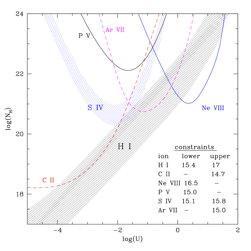
Figure 7: Curves of constant ionic column density plotted on the plane of total hydrogen column density ($N_{\scriptscriptstyle H}$) of the slab vs. the ionization parameter of the incident radiation ($U$), using solar abundances. Lower limits are shown as solid lines, upper limits as dashed lines, shaded regions designate cases where we have both limits for a given ion. The inserted Table gives the $\log(N_{ion})$ for the various constraints.

Several important conclusions can be drawn from Figure 7. The combined constraints from H i, S iv, C ii, Ar vii as well as from other available CNO ions (which for clarity’s sake are not shown here), suggest that the absorber is characterized by $20.3<\log(N_{\scriptscriptstyle H})<20.8$ and $-1.7<\log(U)<-1.2$. This narrow range in the $N_{\scriptscriptstyle H}/U$ plane is fully consistent with 23 out of our 27 ionic column-density constrains, without assuming departure from solar abundances. However, the limits on the allowed metalicity range are rather wide, reflecting the uncertainty in the H i BAL column density (see § 3.4). We find that a simple scaling of the metalicity in our models allows for solutions consistent with the H i constraints for $0.7{\rm Z}_{\odot}<Z_{0946}<10{\rm Z}_{\odot}$. The total column density of the absorber is inversely proportional to its metalicity value.

There are two constraints which are inconsistent with this narrow range in the $N_{\scriptscriptstyle H}/U$ plane. The firm detection of P v (and even more so in the FOS data, see Junkkarinen et al. 1997) yields the associated lower limit on Figure 7, which is incompatible with the allowed parameter space we derived above. The simplest way to resolve this apparent contradiction is to assume that phosphorus is over-abundant by a factor of 10–30 compared to its solar abundance. All else equal, this will lower the P v curve to the point where it intersects with the allowed parameter space. Further discussion of the inferred phosphorus over-abundance is found in § 4.1 and in the Appendix.

Another inconsistency is evident from the Ne viii curve, for which the allowed parameter space is strongly excluded by most other metal constraints. Here there are two possibilities. If the Ne viii measurement is robust, our naive assumption of a single $U$ value (or a narrow range of $U$) must be wrong. A second option is to question the Ne viii detection since the Ne viii BAL resides in the middle of the large trough and is blended with strong O iv, S v and N iv BALs, as well as from a few weaker ones. However, as we show in § 3.4 and in Figure 6 it is very probable that the wide absorption trough around 750 Å contains a considerable Ne viii BAL contribution. The constraints from S vi and Ne v are also marginally above the allowed area in the $N_{\scriptscriptstyle H}/U$ plane (by $\sim 0.2$ dex). Since both ions are of relatively high ionization potential, these results support the hypothesis of a larger range of higher $U$ values in the outflow, which is needed to explain the inferred Ne viii value. We also point out that the uncertainties in the continuum’s shape increase at higher energies (since our last data point lies near 1.8 Ry). Therefore, in the vicinity of these high ionization potentials the extrapolated flux level is rather uncertain, which may contribute to the inconsistency between the model results and the observed constraints for these ions.

How relevant are these constraints to the actual PG 0946+301 outflow? Our analysis of the FOS data (FOS99) suggests a range in the ionization parameter at a given velocity. Furthermore, it shows that the velocity dependence of the apparent optical depth is different for low ionization BALs than for high ionization ones (some of this is accounted for by using different templates for high vs. low ionization species). We argue that these effects can only modestly change our overall IEA conclusions, but there might be some minor outflow components with differing constraints which are missed by ignoring the velocity dependencies. Several arguments support this assertion. The P v relative ionic fraction is at a maximum inside the $U$ range already derived from the other metals/hydrogen constraints, $-1.7<\log(U)<-1.2$. Therefore, a wide range in $U$ will only increase the inferred over-abundance of phosphorus. More generally, inspection of the H i and S iv constraints shows that a similar conclusion applies for most metals. It is difficult to construct a multi $U$-zone model which will reproduce a better S iv to H i ratio without invoking a larger departure from solar metalicity for both higher and lower $U$ models.

For comparison, using the MF spectrum for the same analysis presented in Figure 7 leads to the following conclusions: The absorber is characterized by $19.8<\log(N_{\scriptscriptstyle H})<20.3$ and $-2<\log(U)<-1.5$ and a minimum metalicity enhancement of 2-3 compared to solar. The metalicity enhancement is necessary since for the MF spectrum the strips allowed by the S iv and H i constraints do not overlap, and most of the metals’ lower limit curves lie somewhat above the allowed H i zone.

4.1 The Phosphorus Over-abundance

Previous claims for a large phosphorus over-abundance in PG 0946+301 are found in Junkkarinen et al. (1997). By comparing the derived column densities of C iv and P v and accounting for possible ionization differences, these authors derived (P/C)${}_{0946}\sim 60$(P/C)_⊙. However, this assertion is crucially dependent on the assumption that the column densities deduced from converting the residual intensities to optical depth are a good approximation for the real ones. Even at the time, the possibility of saturation and covering factor was addressed and Junkkarinen et al. acknowledged that: “If the C iv column density is underestimated by a large factor and the P v column density is underestimated by a small factor, then the apparent over-abundance of phosphorus could be much less.” Since there is now ample evidence for saturation and varying covering factor in the BALs of PG 0946+301, the phosphorus over-abundance claim based on the P v/C iv ratio cannot stand on its own.

Our claim for a phosphorus over-abundance does not suffer from this weakness since we do not treat apparent $N_{ion}$ (i.e., the template fitting values) as real $N_{ion}$. Instead we use $N_{ion}$ lower and upper limits, which are largely immune to saturation and covering factor effects. As can be seen in Figure 7 a comparison between the P v lower limit and the H i upper limit necessitates a large phosphorus over-abundance in order for the two constraints to overlap in parameter space. The exact value will depend somewhat on the shape of the ionizing continuum and on the spread of $U$ values, but a phosphorus over-abundance by a factor of less than 10 relative to solar requires a rather contrived photoionization model. We also checked whether optically thick (bound-free) photoionization models could ease or eliminate the need for phosphorus over-abundance. Our conclusion is that these models do not improve on the optically thin results, where the details of this investigation are found in the Appendix.

Finally, it must be noted that there remain major uncertainties in some of the atomic physics implemented in spectral simulation codes such as Cloudy. Among these are many of the dielectronic recombination coefficients, especially for 3rd and 4th row elements, such as P, S, and Ar (see Ferland et al. 1998). Until more reliable coefficients become known, any conclusions drawn regarding gas abundances of these elements should be done so with caution.

5 SUMMARY

We have presented an HST/STIS spectrum of PG 0946+301, which constitutes the highest quality UV data set of any BALQSO. These data are both high signal to noise and covers a very large number of BALs between 500 Å and 1550 Å in the rest frame. This provides for much tighter constraints on the ionization and abundances than previously possible. These data are available to the community for further analyses at:
http://unix.cc.wmich.edu/korista/ftp/pg0946/spectra

Our preliminary analysis of these data yield the following results:

• Most of the 27 BAL troughs detected are saturated while not black (i.e., their shape is largely determined by partial covering effects).

• The main outflow component is characterized by a total column density $20.3<\log(N_{\scriptscriptstyle H})<20.8$, ionization parameter $-1.7<\log(U)<-1.2$ and is consistent with solar abundances. However, the metalicity can be up to ten times solar due to the large uncertainty in the H i BAL column density. These findings take into account the complications posed by the saturation mentioned above.

• The abundance ratio of phosphorus to other metals is roughly ten times the solar ratio. Ionization models including a He ii ionization front cannot significantly decrease the necessary phosphorus over-abundance.

• In addition to the main outflow component, a much higher ionization component appears to be present. This wide range in ionization parameter is inferred from the detection of Ne viii and supported by the constraints from other high ionization species.

• A new shallow high velocity trough appeared in these spectra that was not present in the 1992 HST/FOS spectra. This trough is evident only in the higher ionization lines, and the depth of this trough appears to increase with ionization potential of the ion. Significant changes in depth occurred in the main trough as well.

APPENDIX: CAN MODELS WITH IONIZATION FRONTS LESSEN THE REQUIRED PHOSPORUS OVER-ABUNDANCE?

Due to the significance of a phosphorus over-abundance, we made efforts to check whether optically thick (bound-free) ionization models can explain the observed $N_{ion}$ constraints without invoking departure from solar metalicity ratios. The most promising set of such models are those that include a strong He ii ionization front (Voit, Weymann & Korista 1993), where the incident spectrum is strongly suppressed beyond 54 eV, the ionization potential (IP) of He ii. Such an ionizing continuum may protect P v from photo-destruction (IP=65 eV), while still allowing for the photoionization of H i (IP=13.6 eV) and Si iv (IP=47 eV). In principle this can narrow the gap between the H i and P v curves. Another advantage of such a model is that it might explain the sharp dichotomy we observe between the low ionization species (Si iv, N iii, S iv and H i) and the higher ionization species (C iv, N v, O iv, S vi…), since the He ii ionization potential falls in between these groups. However, a possible problem is that Ar vii should also be protected by a He ii front (although to a lesser extent because of its higher IP of 124 eV), but we do not detect it in the data, and due to the high oscillator strength of the Ar vii $\lambda 585.75$ singlet we obtained a strong constraint on the upper limit of its column density ($<10^{15}$ cm^-2).

In order to test whether He ii ionization front models can eliminate or lessen the need for phosphorus over-abundance, we constructed numorous CLOUDY models with such fronts. Here we give a brief summary of several representative models. We attempted to find solar-abundances CLOUDY models which simultaneously reproduce the inferred upper limits to the column densities for H i, S iv and Ar vii, and the lower limit for the P v column density. Due to the low solar-abundance of phosphorus, CLOUDY models tend to produce higher ratios of H i/P v, S iv/P v and Ar vii/P v compared to the observed values, so that the goal of our modelling is to bring the upper limits of these more abundant species into agreement with the lower limits of P v. The observed column density ratio limits are quite constraining, since the ionization potentials of the other ions bracket the IP of P v (see above).

We let CLOUDY find the optimal model (i.e., finding a minimum for the $\chi^{2}$ between the observed and model-produced constraints, summed over the four constraints detailed above) by changing $N_{\scriptscriptstyle H}$ and $U$. The main difficulty is due to the unknown shape of the incident ionizing continuum. We experimented with many continuum shapes and results from four representative models are shown in Table 3: 1) The canonical Mathews and Ferland (MF) AGN spectrum. 2) The $F_{\nu}\propto\nu^{-2}$ ionizing spectrum described in § 4. 3) A very steep spectrum of $F_{\nu}\propto\nu^{-3.5}$ above 1 Ry, which, although not realistic, comes closest to being consistent with the observed column density ratio limits 4) A more physically realistic version of the above, which takes into account the observed $\nu^{-2}$ spectral slope and connects to the MF spectrum at high and low energies.

As can be seen in the table, the column density ratios of Ar vii and S iv to P v are 5–10 times higher than observed. The main reason for this is that if a slab of gas contains a He ii front there are at least two ionization zones present: a zone with highly ionized gas in which He is completely ionized (the He ii Strom̈gren layer), and a second zone behind it in which He ii becomes the dominant helium ion. The first highly ionized zone contains a significant amount of Ar vii. The spectrum irradiating the second zone contains a He ii edge, and this zone contains virtually all of the P v. Due to the high $U$ values of the models (necessary in order not to over produce H i) the first zone is so thick that the Ar vii column density constraint is already exceeded at a total hydrogen column density at which no detectable P v is predicted. If the models try to lower $U$ in order to produce less Ar vii before the front, then too much H i and S iv are produced. The end result is a compromise that keeps both Ar vii/P v and S iv/P v ratio about an order of magnitude above the observed values. Only a very contrived ionizing spectral shape can change this situation. We note that if the outflowing gas sees an ionizing spectrum which already includes a strong He ii front, it is possible to satisfy all four observational constraints. However, in that case we should see evidence for the “shield” that created the He ii front in the spectrum. Since such a “shield” is very probably static, we should see deep absorption features corresponding to it in C iv, N v and O vi, close to the systemic velocity. Such features are not detected in the spectrum.

Table 3: photoionization models with He ii fronts

#	spectral shape	$\log(N_{\scriptscriptstyle H}$)	$\log(U)$	$\tau_{\scriptscriptstyle H\,{\sc i}}$	$\tau_{\scriptscriptstyle He\,{\sc ii}}$	$\frac{\mbox{Ar\,{\sc vii}}}{\mbox{P\,{\sc v}}}$	$\frac{\mbox{S\,{\sc iv}}}{\mbox{P\,{\sc v}}}$	$N_{\scriptscriptstyle H\,{\sc i}}$
1	MF	21.46	-1.1	1.3	190	10	4	$2\times 10^{17}$
2	$\alpha=-2$	21.67	-0.85	0.9	460	10	9	$1.4\times 10^{17}$
3	$\alpha=-3.5$	21.54	0.00	0.1	330	4	4	$1.4\times 10^{16}$
4	$\alpha=-2,-3.5$	21.52	-0.76	0.5	290	6	6	$8\times 10^{16}$

References

- (1)
- (2) Arav, N., & Li, Z. Y. 1994, ApJ, 427, 700
- (3) Arav, N., Li, Z. Y., & Begelman, M. C. 1994, ApJ, 432, 62
- (4) Arav, N., 1996, ApJ, 465, 617
- (5) Arav, N., 1997 in Mass Ejection from AGN, ASP Conference Series, Vol. 128, ed. N. Arav, I. Shlosman, and R. J. Weymann, p. 208
- (6)
- (7) Arav, N., Korista, T. K., de Kool, M., Junkkarinen, V. T. & Begelman, M. C. 1999, ApJ, 516, 27. (FOS99)
- (8)
- (9) Arav, N., Becker, R. H., Laurent-Muehleisen, S. A., Gregg, M. D., White, R. L., Brotherton, M. S., & de Kool, M. 1999, ApJ, 524, 566 (1999b)
- (10)
- (11) Arav, N., Brotherton, M. S., Becker, R. H., Gregg, M. D., White, R. L., Price, T., Hack, W. 2001, ApJ, 546, 140
- (12)
- (13) Barlow, T. A., 1997 in Mass Ejection from AGN, ASP Conference Series, Vol. 128, ed. N. Arav, I. Shlosman, and R. J. Weymann, p. 13
- (14)
- (15) Brotherton, M. S., Arav, N., Becker, R. H., Tran, H. D., Gregg, M. D., Laurent-Muehleisen, S. A., White, R. L., & Hack, W. 2001, ApJ, 546, 134
- (16)
- (17) Churchill, C. W., Schneider, D. P., Schmidt, M., Gunn, J. E., 1999, AJ, 117, 2573
- (18)
- (19) Cohen, M. H., Ogle, P. M., Tran, H. D., Vermeulen, R. C., Miller, J. S., Goodrich, R. W., & Martel, A. R. 1995, ApJ, 448, L77
- (20)
- (21) Crenshaw, D. M., Kraemer, S. B., 1999, ApJ, 521, 572
- (22)
- (23) de Kool, M., & Begelman, M.C 1995, ApJ, 455, 448
- (24) de Kool, M., 1997 in Mass Ejection from AGN, ASP Conference Series, Vol. 128, ed. N. Arav, I. Shlosman, and R. J. Weymann, p. 233
- (25)
- (26) de Kool, M., Arav, N., Becker, R. H., Laurent-Muehleisen, S. A., White, R. L., Price, T., Gregg, M. D. 2001, ApJ, in press
- (27) Ferland, G. J., 1996, University of Kentucky Department of Physics and Astronomy Internal Report
- (28)
- (29) Ferland, G.J., Korista, K.T., Verner, D.A., Ferguson, J.W., Kingdon, J.B., & Verner, E.M. 1998, PASP, 110, 761
- (30)
- (31) Foltz, C. B., Chafee, F. H., Hewett, P. C., Weymann, R. J., & Morris, S. L. 1990, BAAS, 2, 806
- (32)
- (33) Hamann, F. 1997, ApJS, 109, 279
- (34) Korista, K.T., Weymann, R.J., Morris, S.L., Kopko, M., Turnshek, D.A., Hartig, G.F., Foltz, C.B., Burbidge, E.M., & Junkkarinen, V.T. 1992, ApJ, 401, 529
- (35) Korista, T. K., Hamann, F., Ferguson, J., & Ferland, G. J. 1996, ApJ, 461, 645
- (36) Junkkarinen, V.T., Beaver, E.A., Burbidge, E.M., Cohen, R.D., Hamann, F., & Lyons, R. W., 1997, in Mass Ejection from AGN, ASP Conference Series, Vol. 128, ed. N. Arav, I. Shlosman, and R. J. Weymann, p. 220
- (37) Junkkarinen, V.T., Burbidge, E.M. & Smith, H.E 1983, ApJ, 265, 51
- (38)
- (39) Lindler, D. 1998, CALSTIS Reference Guide (CALSTIS Version 5.1)
- (40)
- (41) Kaiser, M.E., et al. 1998, PASP, 110, 978
- (42)
- (43) Mathews, W. G., & Ferland, G. J. 1987, ApJ, 323, 456
- (44)
- (45) Mathur, S., Green, P. J., Arav, N., Brotherton, M., Crenshaw, M., deKool, M., Elvis, M., Goodrich, R. W., Hamann, F., Hines, D. C., Kashyap, V., Korista, K., Peterson, B. M., Shields, J. C., Shlosman, I., van Breugel, W., Voit, M., 2000, ApJ, 533L, 79
- (46) Murray, N., Chiang, J., Grossman, S.A., & Voit, G.M. 1995, ApJ, 451, 498
- (47)
- (48) Ogle, P. M., Cohen, M. H., Miller, J. S., Tran, H. D., Goodrich, R. W., Martel, A. R., 1999, ApJS, 125, 1
- (49)
- (50) Proga, D., Stone, J. M., Kallman, T. R., 2000, ApJ, 543, 686
- (51)
- (52) Schlegel, D. J., Finkbeiner, D. P., Davis, M., 1998, ApJ, 500, 525
- (53) Telfer, R.C., Kriss, G.A., Zheng, W., Davidson, A.F., & Green, R.F. 1998, ApJ, 509, 132
- (54) Turnshek, D. A. 1988, in Space Telescope Sci. Inst. Symp. 2, QSO Absorption Lines: Probing the Universe, ed. S. C. Blades, D. A. Turnshek, & C. A. Norman (Cambridge: Cambridge Univ. Press), 17
- (55) Verner, D.A., Verner, E.M., & Ferland, G.J. 1996, Atomic Data & Nuclear Data Tables, 64, 1
- (56)
- (57) Voit, G. M., Weymann, R. J., & Korista, Kirk T. 1993 ApJ, 413, 95
- (58)
- (59) Wampler, E. J., Chugai, N. N., & Petitjean, P., 1995, ApJ 443, 586
- (60)
- (61) Weymann, R. J., Turnshek, D. A., & Christiansen, W. A. 1985, in Astrophysics of Active Galaxies and Quasi-stellar Objects, ed. J. Miller (Oxford: Oxford Univ. Press) 333
- (62) Weymann, R. J., Morris, S. L., Foltz, C. B., & Hewett, P. C. 1991, ApJ, 373, 23
- (63)
- (64) Zheng, W., Kriss, G. A., Telfer, R C., Grimes, J. P., Davidsen, A. F., 1997, ApJ, 475, 469
- (65)