Is the observable Universe generic?

César A. Terrero-Escalante and Alberto A. García

Departamento de Física, Centro de Investigación y de Estudios Avanzados del IPN, Apdo. Postal 14-740, 07000, México D.F., México.

Abstract

Recently an inflationary potential yielding power spectra characterized by a scale-invariant tensorial spectral index and a scale-dependent scalar spectral index was introduced. We analyze here the implications that this potential could have for the large-scale structure formation in the multiverses scenario of eternal inflation.

1 Introduction

The Standard Cosmological Model (SCM) and Standard Particle Model (SPM) provide a framework for successfully describing the evolution of the microworld from the primordial plasma. Nevertheless, in this framework there are no answers to the questions of where that hot soup came from and how were formed such large structures like galaxies clusters and galaxies which, in turn, are necessary to explain the formation of stars, heavy chemical elements and life. To answer these questions it is necessary to go beyond the standard knowledge.

New results of the cosmic microwave background (CMB) observations [1] confirm the inflationary scenario plus gravitational instability as the leading candidate for a theory of large-scale structure formation at our Universe [2]. According to this theory, the fluctuations of matter and space-time that took place during a period of rapidly accelerated expansion in the early Universe [3] seeded the formation of large-scale structure and gave rise to anisotropies in the CMB radiation. The simplest scenario describes this expansion driven by the potential energy of a single real scalar field coined inflaton. The primordial fluctuations are characterized in terms of power spectra of scalar and tensorial perturbations. Different theories for the physics of the early Universe lead to different primordial spectra (different initial conditions for density evolution) and, after evolving for a while, to different distributions of density and temperature anisotropies in the currently observable Universe. Present level of observations accuracy allows a large number of potentials being reliable candidates for the inflationary potential. However, near future measurements to be carried out by satellites Map and Planck [4] promise to reduce this number to a few candidates. Then, it could be possible to obtain some hints about the physics on energies close to the Planck scale if, as we assume throughout this paper, the single scalar field scenario is the dominant feature of the early Universe dynamics.

If several extensions of the SPM can reproduce its features in a equally satisfactory fashion, then the answer to whether our Universe is generic it is related to the answer of how probable is a given SPM extension to be picked out amongst the others. But, even if one can devise a deterministic way of choosing the appropriate SPM extension, different initial values for the inflaton field dynamics will lead to different universes. We shall come back to this point in the next section.

A very plausible outcome of the satellites measurements will be a central constant value for the rate between the tensorial and scalar perturbations amplitudes as well as the possibility of fitting the CMB observations using a scale-dependent scalar index. Recently, a model generating perturbations described by a scale-invariant tensorial spectral index was introduced [5]. This model could be the best fit to near future observations if the scalar index can be fairly approximated by a constant at small angular scales and departs from that behavior at large scales. Taking into account that currently a constant scalar index is typically used to fit the CMB observations, these assumptions for its possible scale-dependence are well based. Thus, the physics corresponding to this potential could be very close to the actual early Universe physics.

In this contribution we assume that the above mentioned inflationary potential has a strong similarity with the actual one and analyze the implications that this similarity would have for the formation of structure in the multiple Universes arising through the mechanism of eternal inflation.

2 Future-eternal inflation

During inflation it is suitable to assume the space-time geometry corresponding to a flat Friedmann-Robertson-Walker universe. Then the inflaton classical equations of motions are given by

$$H^{2} = \frac{\kappa}{3}\left(\frac{\dot{\phi}^{2}}{2}+V(\phi)\right),$$ (1)

$$\ddot{\phi} + 3H\dot{\phi}=-V^{\prime}(\phi)\,,$$ (2)

where $\phi$ is the inflaton, $V(\phi)$ the inflationary potential, $H=\dot{a}/a$ the Hubble parameter, $a$ the scale factor, dot and prime stand for derivatives with respect to cosmic time and $\phi$ respectively, $\kappa=8\pi/m_{\rm Pl}^{2}$ is the Einstein constant and $m_{\rm Pl}$ the Planck mass. Note that for a unique solution of this system it is necessary to set the initial conditions as for $\phi$ as for $\dot{\phi}$.

Combining Eqs. (1) and (2) it is obtained that for inflation to proceed, i.e. for $\ddot{a}>0$, we must have $V>\dot{\phi}^{2}$. Because friction in Eq. (2) is almost constant then, for the inflationary period to be long enough, the potential must be rather flat. Finally, inflation ends when the inflaton reaches the true vacuum (or, as we shall see later, reaches a critical value which triggers the decay of secondary scalar fields) so, inflation must start far enough from the value corresponding to the potential absolute minimum (or from the triggering critical value). That condition seems to impose some tunning of the initial conditions for inflation that it is the kind of problem that the inflationary idea is aimed to solve. This paradox can be resolved if we assume a random initial spatial distribution for the scalar field values. All we need is a finite probability for a tiny patch of the early Universe to have the desired inflaton value. To understand this, we have to consider the scalar field quantum fluctuations. Indeed, being the inflaton a quantum object, the time evolution of the average value of $\phi$ in a region of linear size $d_{H}=H^{-1}$ can be described by,

$$\phi(t+\Delta t)=\phi(t)+\Delta_{cl}\phi(\Delta t)+\delta_{qu}\phi(\Delta t)\,,$$ (3)

where $\phi(t+\Delta t)$ and $\phi(t)$ are the inflaton values at times $t+\Delta t$ and $t$, $\Delta_{cl}\phi(\Delta t)\simeq\dot{\phi}H^{-1}$ and $\delta_{qu}\phi(\Delta t)$ are changes of the inflaton value during a Hubble time, $\Delta t=H^{-1}$, due to the classical motion and quantum fluctuations respectively. The random quantum jump $\delta_{qu}\phi(\Delta t)$ is characterized by a Gaussian distribution with zero mean and standard deviation $\Delta_{qu}\phi\simeq(2\pi)^{-1}H$. Taking into account that $V>\dot{\phi}^{2}$, then, to leading order, $V\simeq H^{2}$ and larger $\left|\phi\right|$ values will allow larger deviations of $\phi$ from the average value. If we assume that in some Hubble regions the inflaton can pick an initial value $\phi^{*}$ such that,

$${\Delta_{qu}\phi(\phi^{*})\over\Delta_{cl}\phi(\phi^{*})}\simeq\frac{1}{2\pi}\frac{H^{2}}{\dot{\phi}}\geq 1\,,$$

then we have a finite probability (of about a 16%) for the negative (positive) quantum contribution to be larger than the positive (negative) classical displacement. The conclusion is that there is a finite probability that in some Hubble regions of the early Universe the overall scalar field motion will be in the direction of larger $\left|\phi\right|$ values, i.e., higher energies. During inflation, larger values of $\left|\phi\right|$ correspond to a larger factor $e^{N}$ ($N$ is known as the efolds number) by which the size of the initial patch is increased. Then, regions where the scalar field rolls upward the potential hill inflate more and after some Hubble times we will have large spatial regions where all the above story can start again. In the remaining regions, where the overall scalar field motion will be in the direction of smaller $\left|\phi\right|$ values, i.e., lower energies, the inflaton eventually will reach the potential minimum (or the triggering critical value) and will give rise to “big bangs” leading to different universes. This way, the general picture involves some regions of the “mother” Universe eternally inflating and a large number of “baby” universes springing to light through “big bang” labor, with their large-scale structures seeded by the inflaton and metrics quantum fluctuations and growing by gravitational instability. In very few words, that is what it is known as (future) eternal inflation [6].

Now, for each one of these “baby” universes the inflaton final roll-down starts at different values of $\phi$ and with different values of $\dot{\phi}$ and, according with Eqs. (1) and (2), it means that the inflationary period will set different initial conditions for the “baby” universes births. Then, there will be universes with different degree of flatness, and/or different degree of homogeneity and isotropy, and/or different rate of expansion, and/or different number of topological defects, and/or different number and spectrum of particles, and/or different large scale-distribution of matter. Summarizing, from the observational point of view (if there is life “there” to make the observations), most of these universes are different each from the other. Thus, the question in our title reduces to which is the probability for a universe like our to exist in the multiverses scenario. One can naively conclude that with an infinite number of births of “baby” universes this probability must be high, but it is not so simple. The point is that, in the definition

$$Probability={number\;of\;universes\;like\;our\over total\;number\;of\;universes}\,,$$

we are dealing with infinite quantities, $\infty/\infty$, i.e., is an ill-defined probability.

3 The model

From measurements of CMB polarization to be done by satellite Planck it could be possible to determine a central constant value for the rate between tensorial and scalar inflationary amplitudes. From this value it is possible to estimate a constant leading order value for the tensorial index [7]. On the other hand, the increased range and resolution of the CMB observations must allow to discern a possible scale-dependence for the scalar index. Taking into account that current use of a constant scalar index, corresponding to a power-law spectrum, yields nice results while fitting the CMB spectrum, it must be expected the scale-dependence of the scalar index to be slender or hidden in the scales out of reach for observations. A potential yielding perturbations with these peculiarities was found in Ref. [5]:

$$V(\phi)=\left\{\begin{array}[]{rcl}\phi(\epsilon_{1})&=&-\frac{2(C+1)}{\sqrt{\kappa}}\frac{1}{\sqrt{1-4\delta}}\left[-\sqrt{1+\sqrt{1-4\delta}}\arctan\left(\frac{\sqrt{2\epsilon_{1}}}{\sqrt{1+\sqrt{1-4\delta}}}\right)\right.\\ &&+\left.\frac{1}{2}\sqrt{-1+\sqrt{1-4\delta}}\ln\left|\frac{\sqrt{2\epsilon_{1}}+\sqrt{-1+\sqrt{1-4\delta}}}{\sqrt{2\epsilon_{1}}-\sqrt{-1+\sqrt{1-4\delta}}}\right|\right]+\phi_{0}\,,\\ &&\\ V(\epsilon_{1})&=&V_{0}(3-\epsilon_{1})\left|\epsilon_{1}^{2}+\epsilon_{1}+\delta\right|^{C+1}\left|\frac{2\epsilon_{1}+1+\sqrt{1-4\delta}}{2\epsilon_{1}+1-\sqrt{1-4\delta}}\right|^{\frac{C+1}{\sqrt{1-4\delta}}}\,,\end{array}\right.$$ (4)

where $V_{0}$ and $\phi_{0}$ are integration constants, $C\equiv\gamma_{\rm E}+\ln 2-2\approx-0.7296$, $\delta\equiv n_{T}/2$, and $n_{T}=const.<0$ is the tensorial spectral index. The parameter $\epsilon_{1}$ defined by [8, 2],

$$\epsilon_{1}\equiv{{\rm d}\ln d_{\rm H}\over{\rm d}N}=3{\frac{{\dot{\phi}}^{2}}{2}\over\frac{{\dot{\phi}}^{2}}{2}+V(\phi)}\,,$$ (5)

measures the logarithmic change of the Hubble distance per e-fold of expansion and during inflation is restricted to the interval $\epsilon_{1}\in[0,1)$. In fact, in Ref. [5] it was shown that this potential is actually inflationary in only two

Figure 1: Plots of the potential branches, $V_{I}$ (left) and $V_{II}$ (right).

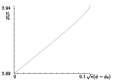
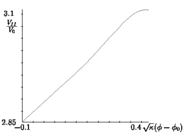
branches corresponding to two different intervals of values for $\epsilon_{1}$, namely, $I=[0,\epsilon_{1}^{+})$ and $II=(\epsilon_{1}^{+},\epsilon_{1}^{*}]$, where $\epsilon_{1}^{+}$ and $\epsilon_{1}^{*}$ are some constant values. A plot of these branches is presented in Fig. 1, where a value of $\delta=-0.01$ was used. In this figure the potential is scaled by $V_{0}^{-1}$ and the scalar field by $\sqrt{\kappa}$. Let us note that, for $V_{I}$ and $V_{II}$, $\epsilon_{1}(t)\rightarrow\epsilon_{1}^{+}$ is reflected in the inflaton asymptotically rolling down toward the origin.

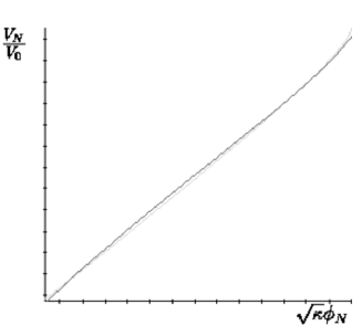
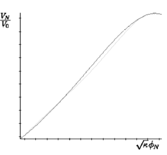
For this model the amplitudes of the scalar perturbations as a function of scales can be also given parametrically. The scales depend on $\epsilon_{1}$ as,

$$k=k_{0}\left|\epsilon_{1}^{2}+\epsilon_{1}+\delta\right|^{\frac{C+1}{2}}\left|\frac{2\epsilon_{1}+1+\sqrt{1-4\delta}}{2\epsilon_{1}+1-\sqrt{1-4\delta}}\right|^{\frac{3(C+1)}{2\sqrt{1-4\delta}}}\,,$$ (6)

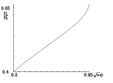
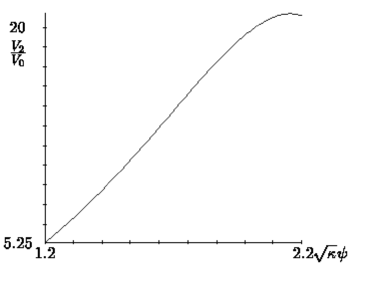
where $k_{0}$ is an integration constant. In turn, the scalar amplitudes normalized by the integration constant $A_{0}$ are given by,

$$\ln\frac{A_{S}(\epsilon_{1})^{2}}{A_{0}^{2}} = \frac{\delta\,C-1-C}{C+1}\ln\epsilon_{1}+\delta\left(C+1\right)\ln\left|\epsilon_{1}^{2}+\epsilon_{1}+\delta\right|$$ (7)

$$+\ \frac{3\delta\left(C+1\right)}{\sqrt{1-4\,\delta}}\ln\left|\frac{2\,\epsilon_{1}+1+\sqrt{1-4\,\delta}}{2\,\epsilon_{1}+1-\sqrt{1-4\,\delta}}\right|$$

$$+\ \frac{\epsilon_{1}^{3}+2C\epsilon_{1}^{2}+2C\delta}{2\left(C+1\right)\epsilon_{1}\,}\,.$$

Figure 2: $\ln A^{2}_{S}$ as a function of the $\ln k$ for $\delta=-0.01$ and for $\epsilon_{1}\in I$ (lower branch) and $\epsilon_{1}\in II$ (upper branch).

As observed in Fig. 2, where the parametric plots of scalar amplitudes for $\epsilon_{1}\in I$ and $\epsilon_{1}\in II$ is presented in the same figure, differences are almost impossible to note when the full range of scales is considered. The strong similarity at small angular scales (large $k^{-1}$) is given by the asymptotic behavior $\epsilon_{1}\rightarrow\epsilon_{1}^{+}$. At these scales, both spectra are very similar to a power-law. Differences from power-law arise at large angular scales (small $k^{-1}$) which could be out of reach for measurements. Now, could this potential be related to any physics? First, our model lacks a graceful exit into the SCM, i.e., there is no “natural” way out of inflation here. To solve this problem, $\phi$ can be regarded as the dominant scalar field in a hybrid scenario with $\epsilon_{1}^{+}$ being the value corresponding to the critical value of $\phi$ near which the false vacuum becomes unstable and the multiple scalar fields roll to the true potential minimum [2, 9]. Next, we note that we cannot make any statement about the potential beyond the intervals $I$ and $II$ [5]. Then, we can only try to check if the forms of the branches $V_{I}$ and $V_{II}$ in Fig. 1 arise in any known physics.

Figure 3: Plots of potentials $V_{1}$ (top, left) and $V_{2}$ (top, right). Bottom: plots superposition; left, $V_{I}$ and $V_{1}$; right, $V_{II}$ and $V_{2}$.

In Fig. 3 we plotted the potentials $V_{1}$ and $V_{2}$ given by,

$$\frac{V_{1}}{V_{0}}=1+e^{1.1\psi}\left(1.1\psi^{2}-0.1\psi^{4}-0.01\psi^{6}\right)+0.001\ln\psi\,,$$

and

$$\frac{V_{2}}{V_{0}}=1-\frac{1}{2}e^{0.7(1-\psi)}\left(1-\psi\right)^{\frac{1}{4}}\,,$$

at given ranges of the scalar field $\psi$. These potentials resemble a hybrid inflation model ($V_{1}$) and a mutated hybrid inflation model ($V_{2}$) which have well motivated particle physics behind. The new feature here are the factors $\exp{\alpha_{i}\phi}$ (with $\alpha_{i}$ some constants) that can be regarded like running couplings (see report [10] for details and references about similar models). In the bottom of Fig. 3, superposition of $V_{I}$ with $V_{1}$, and $V_{II}$ with $V_{2}$ are plotted, after conveniently renormalizing the potentials and scaling and shifting the scalar fields. It can be observed that an opportunity window is open for potential (4) being linked to an (exotic) extension of the SPM. We use this admittedly ad hoc argument just to note that physics described by potential (4) deserve more attention than if it was merely a nice tool to fit the observational data.

4 Generic or not?

There is no reason to assume a stochastic initial distribution for $\phi$ and not for $\dot{\phi}$. According to Eq. (5), starting with random $\phi$ and $\dot{\phi}$ means starting with random $\epsilon_{1}$ then, in the beginning, in some Hubble regions the inflaton is located in branch $V_{I}$, and in some other Hubble regions, in branch $V_{II}$. Hence, in the subset of these regions where the roll-up the potential will eventually dominate, different high energies physics will be set up. Now, while rolling down, $\Delta_{qu}\phi$ decreases and, due to the uncertainty principle, the equal-time standard deviation for the canonical conjugate of $\phi$, i.e., $\Delta_{qu}\dot{\phi}$ must increase. Taking into account the asymptotic behavior at these energies, $\epsilon_{1}\rightarrow\epsilon_{1}^{+}$, any quantum perturbation of the canonical momentum $\dot{\phi}$ (translated into quantum perturbation of $\epsilon_{1}$) makes possible that the inflaton “jumps” from branch $V_{I}$ to branch $V_{II}$ and vice versa. This way, memories from the corresponding high energies physics will be smoothly erased. Moreover, this asymptotic behavior of $\epsilon_{1}$ ensures that most of the quantum fluctuations were produced close to the end of inflation. These are the perturbations which play the most important role from the point of view of large-scale structure formation. As we have already seen, at these scales, the scalar spectrum produced while rolling down $V_{I}$ or $V_{II}$ are almost identical to a power-law spectrum.

5 Conclusions

If the branched potential with scale-invariant tensorial spectral index has something to do with reality, then the “baby” universes in the eternal inflation picture will be very similar each to the other from the observational point of view. It means that our Universe will be a generic outcome of the cosmological evolution rather than some extraordinary event. These conclusions can break down if any of the assumptions behind our calculations occurs to be feeble. In our opinion, the weighty but arguable assumptions here are a constant tensorial spectral index, the second order precision of the Stewart-Lyth expressions for the spectral indices, and a semi-classical analysis close to the Planck era. A study is in process to find out to which extent a change in any of these assumptions changes our conclusions.

Acknowledgments. We are grateful to J. E. Lidsey, E. J. Copeland and R. Abramo for useful discussions. This work is supported in part by the CONACyT grant 32138–E and the Sistema Nac. de Investigadores (SNI).

References

- [1] C. B. Netterfield et al., astro-ph/0104460; A. T. Lee et al., astro-ph/0104459; N. W. Halverson et al., astro-ph/0104489. C. Pryke et al., astro-ph/0104490.
- [2] A. Linde, Particle Physics and Inflationary Cosmology (Harwood, Chur, Switzerland, 1990); A. R. Liddle and D. H. Lyth, Cosmological Inflation and Large-Scale Structure (Cambridge University Press, Cambridge, UK, 2000).
- [3] A. A. Starobinsky, Pis’ma Zh. Eksp. Teor. Fiz. 30, 719 (1979) [JETP Lett. 30, 682 (1979)]; V. Mukhanov and G. Chibisov, Pis’ma Zh. Eksp. Teor. Fiz.33, 549 (1981) [JETP Lett. 33, 532 (1981)]; A. Guth and S. Y. Pi, Phys. Rev. Lett. 49, 1110 (1982); S. Hawking, Phys. Lett. 115B, 295 (1982); A. A. Starobinsky, Phys. Lett. 117B, 175 (1982).
-
[4]
Microwave Anisotropy Probe (MAP) http://map.gsfc.nasa.gov/;
Planck http://astro.estec.esa.nl/SA-general/Projects/Planck/. - [5] C. A. Terrero-Escalante, E. Ayón-Beato, and A. A. García, Phys. Rev. D 64, 023503 (2001).
- [6] P. J. Steinhardt, in The Very Early Universe, Proc. Nuffield Workshop, 21 june - 9 July, 1982, eds: G. W. Gibbons, S. W. Hawking, and S. T. Siklos (Cambridge Univ. Press, 1983), p. 251; A. Vilenkin, Phys. Rev. D 27, 2848 (1983); A. D. Linde, Mod. Phys. Lett. A1 81 (1986); A. D. Linde, Phys. Lett. 175B, 395 (1986); A. H. Guth, Phys. Rep. 333 555 (2000).
- [7] M. Kamionkowsky and A. Kosowsky, Ann. Rev. Nucl. Part. Sci. 49, 77 (1999).
- [8] D. J. Schwarz, C. A. Terrero-Escalante, and A. A. García, astro-ph/0106020.
- [9] A. D. Linde, Phys. Lett. 249B, 18 (1990); A. D. Linde, Phys. Lett. 259B, 38 (1991).
- [10] D. H. Lyth, A. Riotto, Phys. Rep. 314 1 (1998).