The LBDS Hercules sample of mJy radio sources at 1.4 GHz – II. Redshift distribution, radio luminosity function, and the high-redshift cut-off

Abstract

A combination of spectroscopy and broadband photometric redshifts has been used to find the complete redshift distribution of the Hercules sample of millijansky radio sources. These data have been used to examine the evolution of the radio luminosity function (RLF) and its high-redshift cut-off.

We report the results of recent spectroscopic observations of the Hercules sample, drawn from the 1.4 GHz Leiden-Berkeley Deep Survey (LBDS) with a flux-density limit of 1 mJy. New redshifts have been measured for eleven sources, and a further ten were detected in continuum emission from which upper limits to the redshift are given, derived from the absence of a Lyman-limit break in their spectra. The total number of sources with known redshifts in the sample is now 47 (65%). We calculated broadband photometric redshifts for the remaining one-third of the sample, using a two-component (old stellar population plus starburst) spectral synthesis model.

We use the resulting redshift distribution of this complete sample to investigate the cosmological evolution of radio sources. For the luminosity range probed by the present study ($P_{\rm 1.4~{}GHz}>10^{24.5}$ W Hz^-1 sr^-1), we use the $V/V_{max}$ test to show conclusively that there is a deficit of high-redshift ($z>2$–2.5) objects.

Comparison with the model RLFs of Dunlop & Peacock (1990) shows that our data can now exclude pure luminosity evolution as a viable description of the cosmological evolution of the RLF. However two of the models of DP90 successfully predict the redshift-dependent evolution of the millijansky population and are approximately consistent with its observed luminosity-dependence. These models, and the RLF deduced by direct binning of the data, both favour a luminosity dependence for the high-redshift cut-off, with lower-luminosity sources ($P_{\rm 1.4~{}GHz}\simeq 10^{24}$ W Hz^-1 sr^-1) in decline by $z\simeq 1$–1.5 while higher-luminosity sources ($P_{\rm 1.4~{}GHz}\simeq 10^{25-26}$ W Hz^-1 sr^-1) decline in comoving number density beyond $z\simeq 2$–2.5.

1 Introduction

It has long been known that the comoving number density of radio sources increases with redshift. Evidence for a subsequent decline in the comoving density of low luminosity radio galaxies at $z\ga 1$ was presented by Windhorst (1984). At high luminosities, Peacock (1985) concluded that there was a reduction in the comoving density of compact, flat-spectrum ($\alpha<0.5$, where $S_{\nu}\propto\nu^{-\alpha}$), radio-loud quasars at $z\ga 2$. Dunlop & Peacock (1990, hereafter DP90) extended that study to lower radio luminosities and steep-spectrum sources, and presented evidence that there is also a peak at $z\simeq 2$ in the density of both steep-spectrum quasars and radio galaxies.

However the reality of the decline or ‘cut-off’ in the radio luminosity function (RLF) at high redshift (which cannot be due to dust obscuration, for example) has been challenged following the discovery of radio galaxies at $z>4$ (e.g., Spinrad, Dey, & Graham 1995; van Breugel et al. 1999). Although limited by small-number statistics, Jarvis et al. (2001) find that the comoving number density of the most powerful ($P_{\rm 1.4~{}GHz}>10^{27}$ W Hz^-1 sr^-1) steep-spectrum sources remains constant between $z\sim 2.5$ and $z\sim 4.5$.

The best way to settle this uncertainty is to determine the redshift distribution of a complete sample of radio galaxies selected at a flux-density limit of $\sim 1$ mJy. This limit is sufficiently faint that, if there is no redshift cut-off, a large fraction of the sources must lie at high redshifts, and yet sufficiently bright that objects selected at this flux density are still predominantly classical radio galaxies rather than low-redshift starbursts [Windhorst et al. 1985, Hopkins et al. 2000].

The Leiden-Berkeley Deep Survey (LBDS) consists of nine high-latitude fields in the selected areas SA28, SA57, SA68 and an area in Hercules. They were surveyed with the Westerbork Synthesis Radio Telescope at 1.41 GHz, reaching a 5-$\sigma$ limiting flux density of 1 mJy (Windhorst, van Heerde & Katgert 1984a). Optical counterparts to the radio sources were found using multi-colour prime focus photographic plates of the fields, taken with the Kitt Peak 4-m Mayall telescope. Identifications were found for 53% of the sources in the full survey, whilst for the Hercules field 47 out of 72 sources were identified (Windhorst, Kron & Koo 1984b; Kron, Koo & Windhorst 1985).

The Hercules field was subsequently observed with the 200-inch Hale Telescope at Palomar Observatory between 1984 and 1988 (Waddington et al. 2000, hereafter Paper I). Multiple observations were made through Gunn $g$, $r$ and $i$ filters over six observing runs. After processing and stacking of the multiple-epoch images, optical counterparts for 22 of the sources were found, leaving only three sources unidentified to $r\simeq 26$ mag. Near-infrared observations have been made of the entire Hercules sample at $K$, yielding 60 (of 72) detections down to $K\simeq 19$–21 mag. Half of the sources have been observed in $H$ and approximately one-third in $J$ (Paper I). Prior to the work reported here, approximately half of the sample had spectroscopic redshifts, which were summarised in Table 4 of Paper I. In this paper, we present additional redshift measurements together with photometric redshift estimates, and then investigate the redshift distribution of the sample.

The layout of the paper is as follows. In section 2 we present the results of our most recent efforts to obtain optical spectra of the radio sources with the William Herschel Telescope. In section 3 we describe the methods that we used to calculate photometric redshifts for the 22 sources for which we do not have a spectroscopic measurement. The complete redshift distribution (spectroscopic plus photometric) is then discussed. Finally, in section 4 we compare the redshift distribution of this millijansky sample with the predictions of the model radio luminosity functions of Dunlop & Peacock (1990), and reconsider the evidence for a redshift cut-off in the RLF. For consistency with earlier papers, unless otherwise stated, a cosmology with $H_{0}=50$ km s^-1 Mpc^-1, $\Omega_{0}=1$ and $\Omega_{\Lambda}=0$ is assumed.

2 Spectroscopic data

2.1 Observations and data reduction

Observations of 7 faint red radio galaxies in the LBDS Hercules sample were obtained with the ISIS spectrograph at the 4.2-m William Herschel Telescope (WHT) at the Observatorio del Roque de Los Muchachos, La Palma, on 1995 June 21–24. On 1997 June 30 – July 3, a further 22 sources were observed with ISIS at the WHT, using the same configuration. ISIS is a double-beam spectrograph – light from the slit is split by a dichroic at 6100 Å, with the blue and red light going into separate channels where the optical coatings and CCD detectors have been sensitised to blue and red wavelengths respectively. Using the R158B & R158R gratings, the total wavelength coverage was 3160–9060 Å with a dispersion of 2.9 Å pixel^-1.

Each observation consisted of between one and six exposures of 1800 s each on the radio galaxy, giving a total integration time of 0.5–3 hours per target. The spectra were initially processed online throughout the night, enabling us to move to the next target as soon as sufficient signal was obtained to determine a redshift. The targets were acquired by blind-offsetting from a nearby star, which was also used to determine the expected position of the source on the CCD. Spectrophotometric standards were observed at the start of each night. Arc spectra, tungsten flat-fields and twilight sky flat-fields were taken at the start and end of each night.

The data were reduced using standard techniques. After bias subtraction and flat-fielding, the one-dimensional spectrum was extracted with the NOAO spectroscopy package apextract. An aperture of 3 arcsec was usually sufficient to contain the whole object, while keeping the sky to a minimum. Sky apertures of 5–9 arcsec width were defined on each side of the object aperture. For strong continuum sources, the object could be traced along the full length of the dispersion axis with a low-order ($\leq 3$) polynomial, and this trace was used to extract the spectrum. For sources with poor continuum signal, an adjacent observation of an offset or standard star was used to define the trace. For the spectra with the strongest continuum we used optimal extraction, where the pixels were weighted by their variance, but for fainter sources the spectrum was simply added across the spatial axis. For the very faintest targets (particularly some observed in the 1995 run) we used figaro’s polysky application to perform a two-dimensional sky subtraction, and then searched for line or continuum emission in the image without extracting a one-dimensional spectrum.

Removal of the atmospheric absorption features in the red channel of the spectrum was performed using observations of the early-type star G138$-$31a. Each object spectrum was calibrated by first correcting for extinction, and then multiplying by a sensitivity function calculated from observations of the spectrophotometric standard star BD$+$33$\degr$2642. Finally, the calibrated blue and red spectra were combined by taking the mean of the 32-Å overlap region. The calibrations were tested at this stage by applying them to the standard star observations, and examining the quality of the joint at 6100 Å. There was a small discontinuity of about 8% between the blue and red fluxes across the joint of the standard stars. However, this level of photometric accuracy was quite sufficient for this project which was concerned with measuring redshifts rather than accurate fluxes.

Table 1: Redshifts and individual line identifications for the 11 LBDS Hercules sources observed at the WHT.

Source	$\lambda_{\rm obs}$ (Å)	Identification	$z$
Mean Redshift
53W012	3814	He ii 1640	1.326
$1.328\pm 0.001$	4440	C iii 1909	1.326
	5641	Ne iv 2423	1.328
	7981	[Ne v] 3426	1.330
	8682	[O ii] 3727	1.330
53W019	6056	Ca K 3933	0.5400
$0.5415\pm 0.0005$	6117	Ca H 3968	0.5416
	7979	Mg b 5174	0.5421
	7722	[O iii] 5007	0.5422
53W022	5694	[O ii] 3727	0.5278
$0.5279\pm 0.0001$	7428	H$\beta$ 4861	0.5281
	7577	[O iii] 4959	0.5279
	7650	[O iii] 5007	0.5279
53W026	6200	4000-Å break	0.55
$0.55\pm 0.05$
53W027	4803	[Ne v] 3426	0.4019
$0.4027\pm 0.0002$	5227	[O ii] 3727	0.4025
	6822	H$\beta$ 4861	0.4034
	6956	[O iii] 4959	0.4027
	7024	[O iii] 5007	0.4028
53W034	4775	[O ii] 3727	0.2812
$0.2809\pm 0.0001$	6226	H$\beta$ 4861	0.2808
	6353	[O iii] 4959	0.2811
	6411	[O iii] 5007	0.2804
	8389	[N ii] 6548	0.2812
	8406	H$\alpha$ 6563	0.2808
	8432	[N ii] 6583	0.2809
53W048	6587	Ca K 3933	0.6748
$0.6755\pm 0.0003$	6649	Ca H 3968	0.6756
	7208	G-band 4300	0.6763
	8668	Mg b 5174	0.6753
53W065	8151	[O ii] 3727	1.187
$1.185\pm 0.001$	6110	Mg ii 2799	1.183
53W067	6551	[O ii] 3727	0.758
$0.759\pm 0.001$	6927	Ca K 3933	0.761
	6983	Ca H 3968	0.760
	7550	G-band 4300	0.756
53W083	6510	4000-Å break	0.628
$0.628\pm 0.003$
53W089	6093	[O ii] 3727	0.635
$0.634\pm 0.001$	8097	[O iii] 4959	0.633
	8178	[O iii] 5007	0.633

2.2 Results of the spectroscopy

Of the 28 unique sources observed (one source was observed in both runs), 11 have yielded a redshift, 10 were detected in continuum emission but no redshift could be determined, 1 source has a single emission line but no continuum, and 6 sources were not detected. Table 1 lists the redshifts and line identifications for the sources whose redshift has been determined and the spectra are plotted in figures 1 and 2.

Figure 1: WHT spectra of sources in the LBDS Hercules sample for which a redshift was determined. The spectra have been smoothed by 32-Å. ‘X’ denotes a residual feature such as a night sky line or incompletely removed CCD fringes.

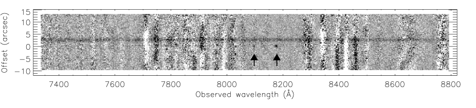
Figure 2: Extract from the two-dimensional WHT spectrum of 53W089. The abscissa is the dispersion axis, with arrows showing the [O iii] 4959 Å and 5007 Å emission lines at $z=0.633$. The ordinate is distance along the slit (to the west), relative to the position of the radio source. The strong continuum emission is from an object 3 arcsec to the west of 53W089. The spectrum has been sky-subtracted but not flux-calibrated; residual sky emission lines are seen as broad vertical bars.

The redshift of 53W026 has been determined from the shape of the continuum (c.f. 53W019) and two possible identifications of the 4000-Å break. The location of the redshifted break is uncertain as it falls within the noisy part of the spectrum where the blue and red halves were joined, and we assign a redshift of $0.55\pm 0.05$ accordingly. No other features could be consistently identified. The [O ii] emission line in 53W065 is the basis for its redshift of 1.185, as this is the only strong feature in the spectrum. There is an absorption feature at 6110 Å consistent with it being Mg ii at the same redshift, but this is at the joint between the two halves of the spectrum and its reality is thus suspect. 53W083 has a very clear 4000-Å break redshifted to 6510 Å putting it at $z=0.628$, but no other features could be identified in the spectrum.

The only source for which a redshift was determined from its two-dimensional spectrum was 53W089 at $z=0.634$. The [O iii] lines at restframe wavelengths 4959 Å and 5007 Å are clearly visible in the sky-subtracted spectrum (figure 2). An [O ii] emission line was also detected in the image. The expected position of H$\beta$ (usually associated with [O iii]) is in a region of the spectrum that is dominated by fringing and the line was not detected.

Ten sources had sufficient continuum flux to enable a strong upper limit to be placed on the wavelength of the 912-Å Lyman-limit break. (Below 912 Å there is essentially no flux in a galaxy’s spectrum due to absorption of the ionizing radiation by H i.) This enables upper limits to be placed on the redshifts of these sources, which are listed in table 2. For one of these sources (53W069) a spectrum was subsequently obtained at the Keck telescope, yielding a redshift of 1.432 [Dey 1997, Dunlop 1999]. Two of the objects (53W013 and 53W021) were barely detected, but most had reasonable flux. Nevertheless, none of these spectra had any lines or breaks that could be successfully identified with known spectral features.

Table 2: Upper limits on the redshifts of sources with continuum flux but no identified spectral features in the WHT observations.

Source	$\lambda_{\rm min}$ (Å)	$z$
53W013	3860	$<3.2$
53W014	3750	$<3.1$
53W021	6000	$<5.6$
53W029	4500	$<3.9$
53W035	4200	$<3.6$
53W036	3800	$<3.2$
53W042	3200	$<2.5$
53W068	3750	$<3.1$
53W069	7200	$<6.9$
53W070	3750	$<3.1$

One source (53W060) yielded a possible detection of a single emission line in the two-dimensional spectrum. One can speculate that the line may be either redshifted Ly$\alpha$ at $z=2.661$ or redshifted [O ii] at $z=0.195$ as these are the strongest lines normally observed in active galaxies. With $r\simeq 25.5$ mag the Ly$\alpha$ identification is favoured on the basis of the $r$-band Hubble diagram, however without independent confirmation this is a very uncertain result and has not been included in our analysis.

Two of the six spectroscopic non-detections (53W037 and 53W087) do not have optical counterparts. We observed them anyway, in the hope that we could detect an emission line that may have been washed-out in the broadband observations. Another of the spectroscopic non-detections (53W091) was subsequently observed with the Keck telescope and a redshift of 1.552 was measured [Dunlop et al. 1996, Spinrad et al. 1997].

These results have now brought the total number of redshifts in the LBDS Hercules sample to 47 out of 72 sources (65%). For the 2-mJy subsample (those sources with $S_{\rm 1.4~{}GHz}\geq 2$ mJy, see Paper I), 40 of the 63 sources (63%) have redshifts. The redshift content of the sample is now quite substantial, but our experience has shown that it will only be completed with the new generation of 8-m class telescopes.

3 Photometric redshift estimates

In order to use the Hercules data to investigate the radio luminosity function and redshift cut-off, the redshifts of the remaining sources must be estimated. The most widely used methods of photometric redshift estimation involve fitting the data to either observed or model spectral energy distribution (SED) templates. A review of the techniques and the reliability of the results is given by Hogg et al. (1998). In this section we describe the method used to estimate the redshifts of sources in the LBDS Hercules field, compare the estimates with the known spectroscopic redshifts and then discuss the basic properties of the resulting redshift distribution.

3.1 Estimation method

In order to develop the best method of calculating photometric redshifts, the ideas of several authors were combined and investigated. Galaxy spectra from the new spectral synthesis models of Jimenez et al. (1998, 2001) were used to compute the template SEDs. We found that the estimated redshifts were not sensitive to the choice of initial mass function (IMF) or metallicity, and the spectral synthesis models with Miller-Scalo IMF and solar metallicity were used in the final analysis. A template spectrum was computed by selecting a spectrum of the required age $F_{\lambda}^{\rm old}$, then adding to that a blue component $F_{\lambda}^{\rm blue}$ scaled such that this component is a fraction $f_{5000}$ of the total flux at 5000 Å. Three forms of the blue component were tested: a young stellar population of age 0.03 Gyr, one of age 0.1 Gyr (following Lilly 1989), and a power-law $F_{\lambda}^{\rm blue}\propto(\lambda/5000)^{-2+\alpha}$ with $\alpha=0.2$ (following Dunlop & Peacock 1993).

Intergalactic absorption due to hydrogen systems along the line of sight was modelled as a damping of the flux at wavelengths shorter than Ly$\alpha$, such that $F_{\lambda}(\lambda<1216~{}{\rm\AA})=F_{\lambda 0}e^{-\tau}$, with $\tau=[(1+z)/5.3]^{3}$ [Gunn & Peterson 1965, Madau et al. 1996]. The Lyman-limit discontinuity, due to the weak stellar emission and strong interstellar H i absorption shortward of 912 Å, was modelled by a cut-off of the form $F_{\lambda}(\lambda<912~{}{\rm\AA})=0$. The effects of possible dust absorption either within the galaxy or along the line of sight were not considered – the additional parameters could not be justified, given that each source had on average only four flux measurements for comparison with the models.

The synthetic flux in each filter ($U^{+}griJHK$) was computed by convolving the model spectrum with the appropriate filter response function (computed from the filter transmission, the atmospheric extinction and the quantum efficiency of the CCD detector). The fluxes were then converted to magnitudes using tabulated flux density measurements of the standard stars BD$+$17$\degr$4708 ($gri$ filters) and Vega ($U^{+}JHK$ filters). Synthetic magnitudes were generated for redshifts $0\leq z\leq 5$ in steps of 0.1, blue component fractions $0<f_{5000}<1$ in steps of 0.02, and twenty galaxy ages (0.01–14 Gyr). The set of synthetic magnitudes was compared with the observed magnitudes of each source, using the $\chi^{2}$ statistic. Non-detections were incorporated into $\chi^{2}$ by using the upper limits to their fluxes. For every source, $\chi^{2}$ was evaluated for each combination of the parameters $z$, $f_{5000}$, and the age, yielding values of $\chi^{2}$($z$,$f_{5000}$,age) for each of the three different blue components. The best-fitting parameters and their errors were determined by using the Levenberg-Marquardt minimization technique described in §15.5 of Press et al. (1992). To the extent that the measurement errors are normally distributed, the errors in the fit are then the 68% confidence limits on each parameter separately.

3.2 Comparison with spectroscopic redshifts

Since two-thirds of the Hercules sample have spectroscopic redshifts ($z_{\rm spec}$), the best-fit photometric redshift ($z_{\rm phot}$) can be compared with the true redshift for these sources. This was done by directly comparing $z_{\rm phot}$ with $z_{\rm spec}$ for each source, and secondly, by computing the median, $\langle\Delta z\rangle_{\rm med}$, of $\Delta z=z_{\rm phot}-z_{\rm spec}$ together with the standard deviation about the median, $\sigma_{\rm med}$. Any sources with $\Delta z>2.5\,\sigma_{\rm med}$ were rejected and $\sigma_{\rm med}$ was recomputed. Each redshift estimation method was assessed on the basis of the values of $\langle\Delta z\rangle_{\rm med}$ and $\sigma_{\rm med}$, the number of points rejected ($N_{rej}$) in the second iteration of $\sigma_{\rm med}$, and the proportion of redshifts that were underestimated (since it is the underestimated redshifts that would affect the subsequent analysis of the redshift cut-off most severely).

It became clear from these comparisons that minimizing $\chi^{2}$ over the whole of the parameter ranges produced a very poor result, so we determined which restricted set of parameters produced the best redshift estimates. Several methods were tested. (i) In order to approximate the methods of the HDF groups (e.g. Lanzetta et al. 1996; Sawicki et al. 1997), the number of spectral templates was limited to three, corresponding to E/S0, Sabc & Sd/Irr galaxies. (ii) Following Lilly (1989), the old component was fixed at ages of either 5, 10, 12 or 14 Gyr. (iii) The age parameter at each redshift was limited such that it was less than the age of the universe. (iv) The blue component was restricted to values of $f_{5000}<0.67,\ <0.5$ and $f_{5000}=0$, to exclude the most blue SEDs.

Figure 3: Comparison of the photometric estimates $z_{\rm phot}$ with the spectroscopic redshifts $z_{\rm spec}$ for the 47 sources with known redshifts. (a) Direct comparison between estimated and spectroscopic redshifts. (b) Histogram of their differences. The median difference is $\langle\Delta z\rangle_{\rm med}=0.13$ and the standard deviation about this median is $\sigma_{\rm med}=0.29$.

Of these methods, it was the second one that produced the most accurate results (figure 3) – fixing the age of the old component and fitting to $z$ and $f_{5000}$. Using the maximum available age for the old stellar population (14 Gyr) and taking the blue component to be a 0.1 Gyr stellar population, gave $\langle\Delta z\rangle_{\rm med}=0.13$ and $\sigma_{\rm med}=0.29$. Note that the median difference between photometric and spectroscopic redshifts remains well within the error distribution.

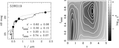
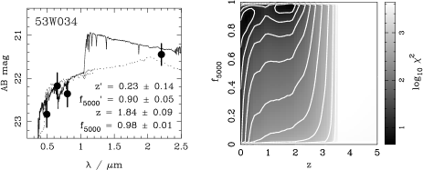
Figure 4: Redshift estimates for 53W019 (top) and 53W034 (bottom). Solid lines denote the best-fitting photometric redshift ($z$), dotted lines denote the redshift ($z^{\prime}$) corresponding to the secondary minimum in $\chi^{2}$. The spectroscopic redshifts are 0.542 and 0.281 respectively.

It can be seen in figure 3 that there are several sources with small spectroscopic redshifts ($z_{\rm spec}\la 0.5$) that are assigned significantly larger photometric redshifts. This effect can also be seen in the work of Lanzetta et al. (1996) and Ellis (1997). In the case of 53W090 at $z_{\rm spec}=0.094$, this is probably due to poor photometry – it is a bright galaxy that extends beyond the apertures used in both the optical and IR images. For the other sources, there appear to be two effects: (i) for $z_{\rm phot}\sim 2$ the location of the 4000-Å break can be anywhere from 1 $\mu$m to 2 $\mu$m due the lack of infrared data at $J$ & $H$; and (ii) for $z_{\rm phot}\sim 3$ the 4000-Å break is being mis-interpreted as the Lyman-limit break at 912 Å. In virtually all cases a second minimum in $\chi^{2}$ is found close to the spectroscopic redshift. Figure 4 illustrates this for 53W019 and 53W034, the two spectroscopic sources which clearly show this effect in figure 3(a). Both these sources have a second minimum in $\chi^{2}$ that differs from their true redshift by $\Delta z<0.1$.

The two sources that have photometric redshifts that are significantly underestimated by this method are 53W009 ($z_{\rm spec}=1.090$) and 53W075 ($z_{\rm spec}=2.150$). Both are classified as quasars and it is perhaps not too surprising that their SEDs are not successfully modelled by a galaxy spectrum. Note, however, that the redshifts of the other four quasars in the sample are correctly estimated.

3.3 Results

The best-fitting model SEDs and the $\chi^{2}$ functions for the twenty-two sources without spectroscopic redshifts are shown in figure 5. Figure 7 presents the likelihood functions $L(z)$ for these sources, normalized to a peak value of unity. The likelihood is defined as $L(z)\propto{\rm exp}(-\chi^{2}(z)/2)$, where $\chi^{2}$ has been minimized with respect to $f_{5000}$, i.e. $\chi^{2}(z)=\chi^{2}(z,f_{\rm min})$ where $f_{\rm min}$ is the value of $f_{5000}$ for which $\chi^{2}$ is a minimum at each fixed $z$. Table 3 lists the best-fitting photometric redshift for each source, together with the one-sigma error $\sigma_{z}$, the blue component fraction $f_{5000}$ and its error $\sigma_{f}$, and the $\chi^{2}$ of the fit. There were typically 2–4 degrees of freedom for each fit, thus it can been seen that most of the $\chi^{2}$ values indicate reasonable fits to the data. Two of the sources (53W051 & 53W070) have a minimum $\chi^{2}$ significantly greater than that required for a good fit, but in both cases this can be attributed to the small photometric errors in the data, rather than any uncertainty in the estimated redshift.

      

      

      

      

      

      

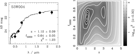
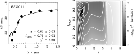
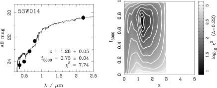
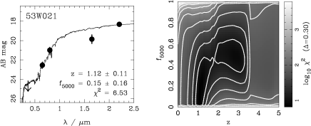
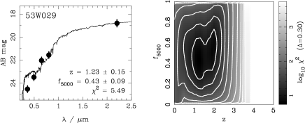
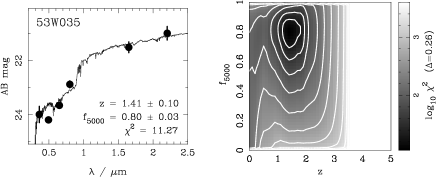
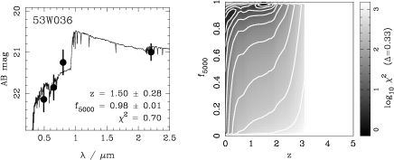
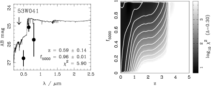
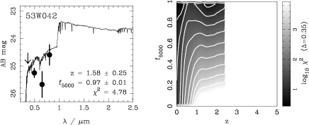
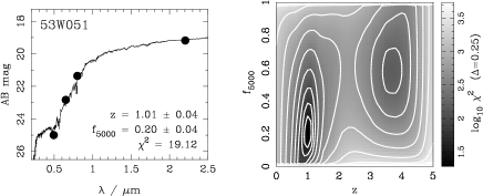
Figure 5: The twenty-two sources in the Hercules sample for which photometric redshifts have been determined. For each source, the best-fitting model SED is shown on the left, together with the observed data points (converted to AB magnitudes); on the right, we plot $\mathop{{\rm log}_{10}}\chi^{2}$ as a function of $z$ and $f_{5000}$. The step size between successive logarithmic contours is given in parentheses ($\Delta$).

      

      

      

      

      

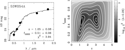
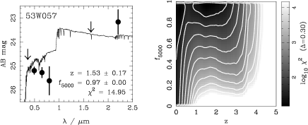
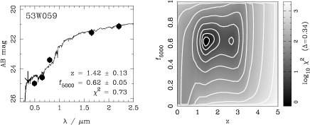
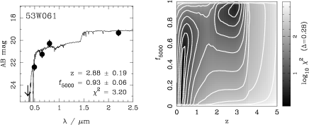
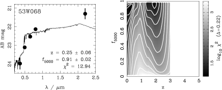
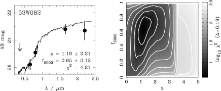
Figure 6: continued

Figure 7: Likelihood functions for the photometric redshifts of the twenty-two sources in the LBDS Hercules sample without spectroscopic redshifts. $L(z)$ has been normalized to a peak value of unity.

Table 3: Photometric redshifts for those twenty-two sources without spectroscopic redshifts. The one-sigma error on $z_{\rm phot}$ is $\sigma_{z}$; $f_{5000}$ is the fraction of the blue component in the spectrum and $\sigma_{f}$ is its error.

Source	$z_{\rm phot}$	$\sigma_{z}$	$f_{5000}$	$\sigma_{f}$	$\chi^{2}$
53W004	1.12	0.09	0.64	0.05	1.23
53W011	0.61	0.03	0.76	0.02	8.58
53W013	1.49	0.22	0.90	0.04	7.82
53W014	1.28	0.05	0.73	0.04	7.74
53W021	1.12	0.11	0.15	0.16	6.53
53W025	0.97	0.17	0.68	0.13	0.59
53W029	1.23	0.15	0.43	0.09	5.49
53W035	1.41	0.10	0.80	0.03	11.27
53W036	1.50	0.28	0.98	0.01	0.70
53W041	0.59	0.14	0.96	0.01	5.90
53W042	1.58	0.25	0.97	0.01	4.78
53W051	1.01	0.04	0.20	0.04	19.12
53W054A	1.25	0.08	0.51	0.06	3.94
53W054B	1.18	0.13	0.91	0.04	3.33
53W057	1.53	0.17	0.97	0.01	14.95
53W059	1.42	0.13	0.62	0.05	0.73
53W060	0.62	0.22	0.95	0.09	5.66
53W061	2.88	0.19	0.93	0.06	3.20
53W066	1.82	0.33	0.91	0.06	1.47
53W068	0.25	0.06	0.91	0.02	12.94
53W070	1.09	0.06	0.21	0.08	35.43
53W082	1.19	0.21	0.65	0.12	4.21

For those sources which have an upper limit to the redshift based on a continuum detection in the spectrum (table 2), this limit was incorporated into the determination of $z_{\rm phot}$ and the errors. In fact, the spectroscopic continuum limit modified the estimated redshift of only one source, 53W070, ruling out a high-$z$ minimum in $\chi^{2}$ at $z_{\rm phot}\simeq 3.7$.

It can be seen in figure 7 that several of the sources have two or more distinct peaks in their redshift likelihood function. We generally adopted the most probable redshift (highest peak) unless the alternative redshift was more consistent with the $K$–$z$ or $r$–$z$ relation for the Hercules spectroscopic sample. In this way we have chosen the second highest peak in $L(z)$ to be the correct photometric redshift for two sources: 53W042 and 53W061. With an $r$-band magnitude of 25.7 mag (Paper I), the ‘peak’ at zero redshift for 53W042 cannot possibly correspond to the true redshift of this source; the alternative of $z=1.58$ is prefered. 53W061 was identified as a probable quasar [Windhorst et al. 1984b] and with $K=17.4$ the alternative redshift of 2.88 (with $\chi^{2}=3.2$) seems more reasonable than $z=0.29$ (with $\chi^{2}=1.3$).

Figure 8: Redshift distributions for the LBDS Hercules sample: (a) all the sources; and (b) those sources with $S_{1.4}\geq 2$ mJy. Hatched histograms are the sources with spectroscopic redshifts, outlined histograms are the sources with photometric redshifts. Note that the ordinate is the weighted number of sources – i.e. corrected for primary-beam attenuation and resolution bias.

The redshift distribution of the LBDS Hercules sources is presented in figure 8, for both the full sample and the 2-mJy sample. In this figure the photometric redshifts from table 3 have been combined with the spectroscopic redshifts from table 1 here and table 3 of Paper I. The numbers have been appropriately weighted to correct for the detection biases in the radio data (see Paper I). The median redshift of the full sample is 0.61, and for the 2-mJy sample it is 0.80. Comparing these results with fainter radio surveys at sub-millijansky and microjansky flux density limits, it is seen that the redshift distribution changes very little over more than two orders of magnitude in radio flux [Windhorst et al. 1999]. In particular, radio observations of the Hubble Deep Field down to 9 $\mu$Jy result in a very similar distribution to figure 8(b), with a mean redshift of $\sim 0.8$ [Richards et al. 1998].

Recall that there are three sources in the Hercules sample that are unidentified and therefore do not appear in the redshift distributions (Paper I). 53W043 was obscured by a bright star in the 4-Shooter CCD observations, but a limit of $F^{+}>23$ mag was obtained from the photographic plates. This places a lower limit on its redshift of $z\ga 0.5$. The other two unidentified sources (53W0037 & 53W0087) both have $r\ga 25$ mag, placing them at $z\ga 1$–2. With a combined weight of 3.7, these three sources will not significantly change the distribution but will likely extend the high-redshift tail when they are finally identified. We calculate an upper limit to the median redshift of the whole 72-source sample of 0.63 and an upper limit of 1.09 for the 2-mJy sample, taking into account these unidentified sources.

Figure 9: The luminosity–redshift plane for sources with $S_{1.4}\geq 2$ mJy in the LBDS Hercules field. The flux density limits for the survey are shown for flat-spectrum (solid line, open circles) and steep-spectrum (dashed line, solid circles) sources, together with the limits for the PSR (dotted line) and 3CR (dot-dash line) surveys. Photometric redshifts have been used for those sources without a spectroscopic measurement.

In figure 9 we compare the flux density limits of the LBDS with those of the Parkes Selected Regions (PSR; Dunlop et al. 1989) and 3CR [Laing, Riley & Longair 1983, Spinrad et al. 1985] surveys. It can be seen how the LBDS can be used to: (i) probe the faint end of the RLF out to much greater redshifts than the brighter surveys; and (ii) detect powerful radio galaxies out to very high redshifts ($z\ga 10$). With a flux density limit of $S_{1.4}=2$ mJy, the LBDS is $\sim$100 times fainter than the PSR used by DP90. In the PSR sample, only the most powerful ($\mathop{{\rm log}_{10}}P_{1.4}>26$) sources are detectable at $z>1.5$. The LBDS can detect sources at the same redshift which have luminosities of $\mathop{{\rm log}_{10}}P_{1.4}\simeq 24$ – such sources are below the flux density limit of the PSR for any redshift $z>0.1$. If there is not a high-redshift cut-off in the RLF, then there will be a significant fraction of sources in the LBDS at high redshifts. For example, figure 14(b) of DP90 predicts the cumulative redshift distribution for the whole LBDS sample based on their RLF models. As many as 10% of the sources may have redshifts greater than 3 according to the models, although the predicted distribution was rather poorly constrained beyond $z\ga 0.7$. This ability of the LBDS to confirm or refute the cut-off was one of the motivations to complete the optical identification of the LBDS and to obtain redshifts for as many sources as possible. The lack of sources at $z\ga 2.5$ in figure 9 is striking, and clearly suggests that there is indeed a redshift cut-off in the RLF. In the next section, we quantify this statement and compare the data with the models of DP90.

4 The radio luminosity function and redshift cut-off

4.1 A review of the RLF models

In an extension of work begun by Peacock & Gull (1981) and Peacock (1985), DP90 investigated the evolution of the 2.7-GHz radio luminosity function, with an emphasis on the behaviour of the RLF at high redshift. Their method was to find a model (or rather, an ensemble of models) of the luminosity function $\rho(P,z)$, that was consistent with all the available data. In those regions of the $P$–$z$ plane where the redshift content of the data was high, generally corresponding to the higher flux densities, the model was well defined. The model was then extrapolated across the rest of the $P$–$z$ plane, subject to the constraints of less direct data such as source counts. Of course, it is known that the real universe is not smooth on all scales, so the models will only be approximations to the actual form of the RLF.

The data were drawn from four complete samples at a frequency of 2.7-GHz, together with source counts at fainter flux limits and measurements of the local RLF. The deepest of these samples was the Parkes Selected Regions (Downes et al. 1986; Dunlop et al. 1989), with a flux density limit of 0.1 Jy and containing 178 sources (including a higher proportion of steep-spectrum sources than the other samples). However, only 46% of the PSR sources had redshifts, so DP90 used the empirical $K$–$z$ relation of Lilly, Longair & Allington-Smith (1985) to estimate the redshifts of the remaining 54% of the data.

The ensemble of model RLFs consisted of five ‘free-form’ and two parametric models that were found to be consistent with the data. The free-form models (here denoted by FF-1, $\ldots$, FF-5) are forth- or fifth-order series expansions in $\mathop{{\rm log}_{10}}P_{2.7}$ and $z$, with various forms of high-redshift cut-off imposed on the models. Each of these models was derived twice, using two different estimated redshift distributions (denoted by ‘MEAN-z’ and ‘HIGH-z’). DP90 also fitted their data with two simple parametric models: pure luminosity evolution (PLE) and a combination of luminosity and density evolution (LDE). The PLE luminosity function was modelled as the sum of a low-power non-evolving component (a sixth-order polynomial in $\mathop{{\rm log}_{10}}P_{2.7}$) and a high-power evolving component (a double power-law in $P_{2.7}$, with a break luminosity parameterized as a quadratic function of $z$). The LDE model was a modification of PLE, in which the space density was allowed to vary with redshift directly, in order to investigate the possibility that the cut-off was due to negative density evolution while the positive luminosity evolution continued at $z\ga 2$.

For the flat-spectrum population, a decline in the RLF at high redshifts ($z\ga 2$) is required by the models for all luminosities where the complete sample database has good coverage of the $P$–$z$ plane (the strength of this result is due to the nearly complete redshift data for the flat-spectrum population). For the steep-spectrum sources, a cut-off is required for the most luminous objects ($\mathop{{\rm log}_{10}}P_{2.7}\geq 27$) at $z\ga 2$, and it is consistent with the data at all luminosities. This was the first time that a high-$z$ cut-off in the RLF had been quantified in the steep-spectrum population, although it had also been suggested by the observations of Windhorst (1984).

DP90 also performed a model-independent test of the cut-off using the banded $V/V_{\rm max}$ test [Schmidt 1968, Rowan-Robinson 1968, Avni & Schiller 1983]. For a uniform distribution of objects in space, the mean $\langle V/V_{\rm max}\rangle$ should be 0.5. The banded $V/V_{\rm max}$ test is a function of redshift and enables any high-redshift negative evolution to be separated from the strong, positive evolution at lower redshifts. Applying this test to their complete sample database gave values $\langle V/V_{\rm max}\rangle<0.5$, on average, for the flat-spectrum sources at $z\ga 1$ and for the steep-spectrum sources at $z\ga 1.5$, indicating a deficit of high-redshift objects. At lower redshifts, values of $\langle V/V_{\rm max}\rangle>0.5$ clearly demonstrated the strong positive evolution of both the steep- and flat-spectrum populations at $z\la 1$.

4.2 The cumulative redshift distribution

The models of DP90 were used to extrapolate the RLF to lower radio luminosities and higher redshifts than were sampled by their data. In fact the models predict the form of the RLF over the whole of the $P$–$z$ plane illustrated in figure 9. Thus we can use the LBDS Hercules sample to test the reality of the redshift cut-off found by DP90. As we discussed in Paper I, the large weights of the nine sources with $1\leq S_{1.4}<2$ mJy causes the full sample to be biased towards these low signal-to-noise objects. Throughout this section, therefore, only the 63 sources with $S_{1.4}\geq 2$ mJy (i.e. the ‘2-mJy sample’) will be considered.

Two approaches have been used in order to compare the predictions with the Hercules data. First, the model luminosity functions were used to calculate the expected redshift distribution in the Hercules field, in the form of cumulative number counts. Second, the space density of sources in the sample was calculated as a function of radio luminosity and redshift, to compare directly with the models. This second method has the advantage that the luminosity dependence can be investigated directly, but with only 63 sources in the sample (of which three have no optical counterpart) the sampling and statistics are quite poor. The first method allows more robust conclusions to be drawn, but at the expense of losing the luminosity information.

DP90 divided their data according to spectral index ($\alpha$, where $S_{\nu}\propto\nu^{-\alpha}$), and calculated model RLFs for the steep-spectrum ($\alpha\geq 0.5$) and flat-spectrum ($\alpha<0.5$) populations separately. For their complete samples, spectral indices were known for all sources. However, the data from the fainter samples were generally restricted to source counts, with no spectral index information available. To separate the faint number counts into steep- and flat-spectrum sources, they approximated the flat-spectrum contribution by a model, ${\rm d}n_{\rm flat}/{\rm d}S=45\,S^{-2.5}\,\exp[-(\ln S)^{2}/8]$ Jy^-1 sr^-1, which was then subtracted off the data to give the steep-spectrum counts. These number counts were incorporated into the respective RLF models of the two populations.

It became apparent during the current work that this model for the flat-spectrum contribution at faint flux densities was incorrect. The number of steep-spectrum sources in the Hercules data is significantly lower than the RLF models predicted, and conversely there are more flat-spectrum sources in the data than in the models. The predicted total number of sources (steep- plus flat-spectrum) agreed with the data, as it should. In particular, DP90’s model for ${\rm d}n_{\rm flat}/{\rm d}S$ predicts that there should be 5–10 flat-spectrum sources in the 2-mJy sample, where there are actually 29 of them (after applying the weights for incompleteness). In fact, the ratio of steep-spectrum to flat-spectrum sources is the same in both the PSR and 2-mJy Hercules samples, at approximately 2 : 1 (see also Windhorst et al. 1993; Richards 2000).

We therefore removed the distinction between flat-spectrum and steep-spectrum sources altogether. The data were considered as a single population, and the models were simply added together. Mathematically, this is possible as the RLF models are essentially the number of sources observed in the survey, which can of course be summed. Physically, this is justified by the work of several authors. One of the main conclusions of DP90 was that both populations behave very similarly and may therefore come from a single population. Padovani & Urry (1992) demonstrated that steep- and flat-spectrum radio quasars and FR-II radio galaxies were consistent with being the same physical objects, viewed at different angles and with a range of relativistic beaming parameters (see also Urry & Padovani 1995). Thus in the remainder of this paper we consider a single radio luminosity function for sources of all spectral indices.

The cumulative number counts are calculated for each of the RLFs: five free-form models, PLE and LDE. The total number of sources at redshifts less than $z$ is:

$$N(<z)=\int_{0}^{z}\left[\int_{P_{1}}^{\infty}\rho(P,z)\ {\rm d}P\right]\left({{{\rm d}V}\over{{\rm d}z}}\right){\rm d}z$$ (1)

where $P_{1}$ is the luminosity of a source at redshift $z$ whose flux density would be equal to the detection limit of $S_{2.7}=1.2$ mJy. This projected flux density limit at 2.7 GHz is derived from the flux density limit of the survey at 1.4 GHz (i.e. 2.0 mJy) using the median spectral index of sources in the sample, $\alpha_{\rm med}=0.77$, defined over 0.6–1.4 GHz (Paper I). Equation 1 was evaluated numerically in steps of $\Delta\mathop{{\rm log}_{10}}P=0.025$ and $\Delta z=0.01$. The volume element is ${\rm d}V\simeq\Delta V=[V(z+\Delta z)-V(z)]\Psi$, where the comoving volume of the universe (in Mpc³ sr^-1) out to redshift $z$ is $V(z)$, and $\Psi=3.78\times 10^{-4}$ sr (or 1.22 deg²) is the solid angle of the sample [Windhorst et al. 1984b]. The results are plotted in figure 10. The observed cumulative redshift distribution was computed by summing the weights of the sources from $z=0$ to the redshift of each source in turn. We made a conservative calculation of the uncertainty in this distribution by assuming that all the photometric redshifts were simultaneously at their $\pm 1$-$\sigma$ errors (shaded area in figure 10).

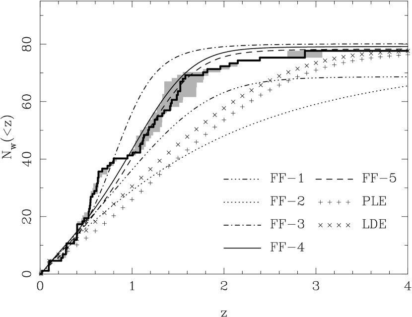
Figure 10: The cumulative redshift distribution of sources in the 2-mJy Hercules sample. The bold histogram is computed from the combined spectroscopic and photometric redshift distribution of the sample. The shaded area is a measure of the uncertainty in the distribution, assuming the photometric redshifts were all at their $\pm 1$-$\sigma$ errors. The model radio luminosity functions of DP90 are also plotted: free-form models 1 through 5 (FF-1, $\ldots$, FF-5), pure luminosity evolution (PLE) and luminosity/density evolution (LDE). $N_{W}$ is the weighted number of sources with redshifts less than $z$.

Five of the models correctly predict the total number of sources in the sample, to within 5%. The weighted number of sources is 81.4, of which 3.7 are unidentified and do not appear in the figure, and the models predict $N_{\rm total}\simeq 78$. The other two models (FF-1 and FF-2) converge to $N_{\rm total}\simeq 73$ by $z=8$.

The best agreement with the data is obtained for free-form models FF-4 and FF-5. At $z<0.5$ and $z>1$ they follow the observed distribution closely. The only disagreement occurs over the range $0.5\la z\la 1$, where the observed redshift distribution rises more rapidly than the models. This rise is due to two peaks in the observed redshift distribution – there are seven sources at $z=0.54\pm 0.02$ and five sources at $z=0.62\pm 0.01$ in the 2-mJy sample (plus another source at $z=0.61$ with $S_{1.4}=1.7$ mJy). These two peaks indicate the existence of large-scale structures (sheets) intersecting the line-of-sight. We suggest that these radio sources may be part of two super-clusters (their comoving transverse separation is $\sim 25$ Mpc), statistical variations that the RLF models could not possibly predict.

With these exceptions, models FF-4 and FF-5 provide a good description of the LBDS Hercules data. Recall that the difference between each of the free-form models lies in the form of the high-redshift cut-off. Although these two models are very similar in their predictions, they were defined somewhat differently. A high-$z$ cut-off was enforced on FF-5 such that the RLF decays sinusoidally from $z=2$ to a value of zero at $z>5$. For FF-4, the model was similarly constrained to a value of zero at $z>5$, but the form of the cut-off was not specified (beyond being smooth and continuous).

The other five models all fit the observed distribution at low redshifts, $z\la 0.4$, where they were relatively well-constrained by the local RLF, but at high-$z$ they fail to match the data (figure 10). The second free-form (FF-2), pure luminosity evolution (PLE) and luminosity/density evolution (LDE) models in particular, predicted that a much greater proportion of the sources would have large redshifts. Using a preliminary version of this sample, Dunlop (1997) found that the PLE and LDE models were consistent with the high-redshift ($z>2$) distribution of the data. However with the additional spectroscopic and photometric redshifts now available, we see that these models show a large disagreement with the data over lower redshifts, $0.5\la z\la 2.5$. This is primarily due to the fact that the improved SED-based redshift estimation procedure used here has proven that the redshifts for many sources were previously over-estimated on the basis of the $K-z$ relation for powerful radio galaxies.

The first of the free-form models (FF-1) approximately follows the redshift distribution from $z=0$ to $z\sim 1$, however the number of sources at higher redshifts is $\sim$15% too low. The third of the free-form models (FF-3) is in reasonable agreement with the data for redshifts $z\la 0.8$, but then continues to rise steeply. It predicts that there should be only five sources at $z>1.5$, which is inconsistent with the data as there are already ten sources with spectroscopic redshifts greater than this.

4.3 The binned radio luminosity function

Figure 10 has shown which models correctly predict the overall redshift dependence of the radio luminosity function, but it says nothing about the luminosity dependence. To investigate this, we calculated the observed RLF to compare directly with the models. This was done by redshift and luminosity binning of the 2-mJy Hercules data. The luminosity of each source at 2.7 GHz (the frequency at which the RLF models are defined) was calculated from the observed flux at 1.4 GHz and the 0.6–1.4 GHz spectral index. Eight luminosity bins were used, from $\mathop{{\rm log}_{10}}P_{2.7}=20$ to 28 in steps of $\Delta\mathop{{\rm log}_{10}}P_{2.7}=1$. Five redshift bins were used, from $z=0$ to 4, centred on $z=0.1$, 0.5, 1.1, 1.7 and 3.0. These redshifts approximately correspond to ages of 90%, 50%, 33%, 25% and 10% of the current age of the universe (for an Einstein-de Sitter cosmology where $(1+z)\propto t^{-2/3}$). The bins were chosen so as to contain enough sources to be statistically useful, while being sufficiently narrow to resolve the redshift dependence of the RLF. The binned luminosity function is presented in figure 11. While the small number of sources is the weakness of this method of analysing the data, its strength lies in the accuracy with which the luminosities are known, given the effectively complete redshift information for the sample.

Figure 11: The observed radio luminosity function for the 2-mJy Hercules sample. The different symbols and lines correspond to different redshifts, as shown, with arrows representing bins which contain a single source. The RLF has been plotted against the 2.7 GHz luminosity of each source (extrapolated from the 1.4 GHz luminosity) to aid comparison with the models.

Given the relatively large width of the redshift bins, an additional weight had to be applied to each source to correct for the fact that the weakest sources could not have been detected at all redshifts within the bin. Specifically, each weight was scaled by $V/V_{\rm lim}$, where $V=V(z_{2})-V(z_{1})$ is the comoving volume enclosed by the bin extending from redshift $z_{1}$ to $z_{2}$, and $V_{\rm lim}=V(z_{\rm lim})-V(z_{1})$ is the volume enclosed from $z_{1}$ to the redshift $z_{\rm lim}$ at which the source would fall below the radio flux density limit of the sample (clearly if $z_{lim}\geq z_{2}$ then this weighting was unnecessary). Errors were assigned to each bin on the basis of Poisson counting statistics, applied to the raw weighted counts before correcting for the flux-density-limit bias.

It is seen in figure 11 that the observed low-redshift RLF evolves more slowly at low luminosities than it does at the higher luminosities studied by DP90. It is not until $z\ga 0.5$ that we see significant evolution in the luminosity bins. At $\mathop{{\rm log}_{10}}P_{2.7}=23.5$, the density of sources at $z=1.1$ (triangles in figure 11) is reduced by an order of magnitude from that in the lower redshift bin at $z=0.5$ (stars). Note that this may be due to incompleteness at the survey limit, but that is unlikely – we showed in Paper I that the sample is effectively complete once the appropriate weights have been applied to the sources. There is no evidence for a declining RLF at the same redshift ($z=1.1$) in the next luminosity bin ($\mathop{{\rm log}_{10}}P_{2.7}=24.5$), suggesting that the cut-off redshift is a function of the radio luminosity.

One of the most significant features in figure 11 is the behaviour of the high-redshift radio luminosity function (encircled crosses). All three points defining the RLF at $z>2$ lie below those of the same luminosities ($\mathop{{\rm log}_{10}}P_{2.7}=24$–27) at $z<2$. In particular, the density of sources with $\mathop{{\rm log}_{10}}P_{2.7}=24.5$ decreases by a factor of six between $z=1.7$ and 3.0. The decline at a luminosity of $\mathop{{\rm log}_{10}}P_{2.7}=25.5$ appears to be less dramatic and is of low formal significance due to there being just a single source at $z=1.7$ at this luminosity. It can be seen that the density has dropped by a factor of ten between $z=1.1$ and 3.0 over this same luminosity interval. We conclude from our direct binning of the RLF that the comoving density of low-luminosity radio sources begins to decline at redshifts $1\la z\la 2$ and that the actual redshift of the turnover may depend on the radio luminosity.

Figure 12: The observed radio luminosity function (points) for the 2-mJy Hercules sample compared with the two model RLFs of DP90 which correctly predicted the redshift distribution of the sample: (a) FF-4, and (b) FF-5.

In figure 12 we compare the observed luminosity function with the two model RLFs of DP90 which correctly predicted the redshift distribution of the sample, i.e. free-form models FF-4 & FF-5. At the lowest redshifts, $z<0.2$ (squares, solid lines in figure 12), the model RLFs are consistent with the data within their errors. At a redshift of $z\sim 0.5$ (stars, dash-dot-dot-dot lines) both models predict too many sources at $\mathop{{\rm log}_{10}}P_{2.7}\simeq 22$–23 and too few at $\mathop{{\rm log}_{10}}P_{2.7}\simeq 24$–26, although the data differ from the models by only a few sigma. At $z\sim 1.1$ (triangles, dashed lines) the data and models are in reasonable agreement at $\mathop{{\rm log}_{10}}P_{2.7}>24$, but there are significantly fewer low luminosity ($\mathop{{\rm log}_{10}}P_{2.7}\simeq 23$–24) sources than predicted.

It is the behaviour of the RLF at the highest redshifts that is crucial for measuring the redshift cut-off. Both the free-form models FF-4 and FF-5 are consistent with the data at $z\sim 1.7$ (filled circles, dotted lines in figure 12), within their two-sigma error bounds. It is seen that at this redshift the model RLFs begin to decline for sources with luminosities $\mathop{{\rm log}_{10}}P_{2.7}<25$, although the observed RLF does not change significantly from $z=0.5$ to 1.7 at these luminosities. The redshift cut-off of DP90 is clearly seen in the highest-redshift bin in figure 12(b) and is even more prominent in figure 12(a). The comoving density of radio sources at $z\sim 3$ is predicted to decline by as much as two orders of magnitude from $z\sim 1.7$. However, the data do not fall off nearly as rapidly as the models. Model FF-5 is closer to the observed RLF than model FF-4 in this high-redshift regime, and is consistent with the data at the two-sigma level.

We noted above that with an average of four sources per binned data point in figures 11 & 12, the statistics are quite poor and the data do not differentiate between the models to a significant degree. However, we have shown that the two models which best fit the observed redshift distribution of the sample are at least consistent with the luminosity dependence of the observed RLF.

4.4 The banded V/V_max test

Following DP90, we applied the banded $V/V_{\rm max}$ test to the Hercules sample in order to investigate the redshift cut-off in a model independent manner. This is a variation of the original $V/V_{\rm max}$ test [Schmidt 1968, Rowan-Robinson 1968], that has been modified to test the evolution of the sample for redshifts greater than some fixed value $z_{0}$. We define $V$ as the comoving volume enclosed by a source at redshift $z$ ($\geq z_{0}$), $V_{\rm max}$ as the volume that would be enclosed by the same object if it were pushed out to the flux density limit of the sample, and $V_{0}$ as the volume enclosed within a redshift of $z_{0}$. If a population of $N$ sources is uniformly distributed for redshifts $z\geq z_{0}$, then $(V-V_{0})/(V_{\rm max}-V_{0})$ would be distributed uniformly between 0 and 1, with a mean of $0.5\pm(12N)^{-0.5}$ [Avni & Bahcall 1980, Avni & Schiller 1983]. Values of the mean $\langle(V-V_{0})/(V_{\rm max}-V_{0})\rangle>0.5$ correspond to an increase in comoving density with redshift, while $\langle(V-V_{0})/(V_{\rm max}-V_{0})\rangle<0.5$ indicates a deficit of high-redshift objects. Note that the values of $\langle(V-V_{0})/(V_{\rm max}-V_{0})\rangle$ do not measure the strength of the evolution directly [Avni & Bahcall 1980], and it would be wrong to use this test to compare the relative rates of evolution at high and low redshifts.

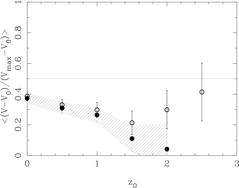
Figure 13: The banded $V/V_{\rm max}$ test for the 2-mJy sample (open circles). The dotted horizontal line indicates the value of 0.5 expected if there is no evolution in the comoving density of sources at redshifts $z>z_{0}$. Values of $\langle(V-V_{0})/(V_{\rm max}-V_{0})\rangle<0.5$ indicate a deficit of high-redshift objects. The solid points show the results of repeating the test after excluding the highest-redshift source, 53W061, whose photometric redshift is uncertain. The hatched region shows the corresponding one-sigma errors.

In figure 13 we present the results of applying this test to the 2-mJy Hercules sample. Over all redshifts, we find $\langle(V-V_{0})/(V_{\rm max}-V_{0})\rangle=0.40\pm 0.03$, differing from the no-evolution line by 3-$\sigma$. The significance of the result remains at $\geq 3$-$\sigma$ for all redshifts $z<2$. At the highest redshifts, $z>2$, the significance is $\sim 1$-$\sigma$, due to the small number of sources (5.4 after weighting). In particular, the highest-redshift source in the sample (53W061 at $z_{\rm phot}=2.88$) is the only object at $z>2.5$, and with a weight of 2.35 it has a disproportionate effect on the test. We illustrate this in figure 13 by removing 53W061 from the sample and repeating the banded $V/V_{\rm max}$ test. The value of $\langle(V-V_{0})/(V_{\rm max}-V_{0})\rangle$ then falls to $0.04\pm 0.17$ at $z>2$. Recall that 53W061 has two peaks in its photometric redshift likelihood function and we chose the high-redshift peak on the basis of its identification as a likely quasar on the Mayall photographic plates. However, it is possible that the source is actually at the lower redshift ($z_{\rm phot}=0.29$); thus excluding it from the $V/V_{\rm max}$ test is not unreasonable.

The small values of $\langle(V-V_{0})/(V_{\rm max}-V_{0})\rangle$ at all redshifts point to a genuine deficit of high-redshift objects in the sample. It doesn’t mean that there is a decline in the comoving density of sources at low redshift, but rather a lack of strong positive evolution at low-$z$ in this population is failing to cancel the high-redshift negative evolution. For example, in the PSR survey (DP90) there is enough positive evolution out to $z>1$ to make the initial banded numbers greater than 0.5, until the negative evolution at high redshift begins to dominate $\langle(V-V_{0})/(V_{\rm max}-V_{0})\rangle$. In the Hercules sample, however, there is little if any positive evolution (compare figure 11) and so the high-$z$ deficit dominates $\langle(V-V_{0})/(V_{\rm max}-V_{0})\rangle$ at all redshifts.

Could the results of the $V/V_{\rm max}$ test be due to something other than a high-$z$ decline in the comoving density of sources? Looking at the values of $V/V_{\rm max}$ for the individual objects shows that 25% of the sample could have been detected at $z>3$, but there are in fact no sources at such redshifts. Comparing the open and solid points in figure 13 suggests that just a few sources at the highest redshifts may remove the evidence for evolution at $z>2.5$. To investigate this we added to the distribution the three unidentified sources, placing them at random redshifts ($0.5<z<3$). This did not change the result of the test; in fact, placing all three sources at $z>2$ actually increased the significance of the negative evolution at the highest redshifts (recall that the error on $\langle(V-V_{0})/(V_{\rm max}-V_{0})\rangle$ goes as $N^{-0.5}$). Therefore the conclusion that there is a significant decline in the source density cannot be falsely attributed to the properties of just a few sources.

Another concern is the effect that spectral curvature may have on the results of the $V/V_{\rm max}$ test. In calculating $V_{\rm max}$ we assumed that the 0.6–1.4 GHz spectral indices of the sources remain constant at higher frequency, but that need not be the case. If the radio spectrum steepens at higher frequencies then the luminosity of a source will be lower than that calculated from the observed spectral index, and the inferred $V_{\rm max}$ will also be smaller. This in turn will give a larger value for $V/V_{\rm max}$. We thus repeated the test after increasing the spectral index of each source ($\alpha\rightarrow\alpha+\delta$, where $S_{\nu}\propto\nu^{-\alpha}$). For reasonable changes in spectral index, $\delta\simeq 1$, the results remain essentially unchanged although the significance drops from 3-$\sigma$ to 2-$\sigma$ at zero redshift. The spectral indices must be increased by $\delta\simeq 3$ before the data become consistent with no evolution at $z<1.5$, and even then values of $\langle(V-V_{0})/(V_{\rm max}-V_{0})\rangle$ $=0.2$–0.3 are found at higher redshifts. Thus the results are robust against spectral curvature.

5 Conclusions

Spectroscopic observations of sources in the LBDS Hercules sample have yielded new redshifts for 11 objects, bringing the redshift content of the sample to 65% (47 of 72 sources). Upper limits to the redshifts of a further 10 sources have been found, based on the absence of a redshifted Lyman-limit break in their spectra.

For the remaining one-third of the sample we have estimated their redshifts from their broadband photometry. After testing several estimation methods on our data, we found that the most accurate results were produced by modelling the spectra as the sum of an old (14 Gyr) stellar population plus a young (0.1 Gyr) stellar population that contributes some fraction ($f_{5000}$) to the 5000-Å flux. Comparing the photometric with the spectroscopic redshift for those sources with a measured redshift showed that our estimates have an accuracy of $\langle\Delta z\rangle_{\rm med}=0.13$ and an rms dispersion of $\sigma_{\rm med}=0.29$, comparable to that of other authors [Hogg et al. 1998].

We have used the combined spectroscopic plus photometric redshift distribution of the 2-mJy Hercules sample to investigate the evolution of the 1.4 GHz radio luminosity function. The 2-mJy sample, which excludes the nine sources with $S_{1.4}<2$ mJy and weights $\ga 3$, has a median redshift of 0.80, comparable to surveys of lower flux density [Richards et al. 1998, Windhorst et al. 1999]. The fact that the redshift distribution hardly changes over two orders of magnitude in radio flux, implies that the faint radio source population must be evolving fairly strongly – the fainter surveys are not simply detecting the same population at a higher redshift. The low-flux density (sub-mJy, $\mu$Jy) surveys are dominated by starbursts, whereas the LBDS survey is dominated by giant elliptical radio galaxies and quasars, at least at $S_{1.4}\ga 3$ mJy [Kron et al. 1985, Windhorst et al. 1999, Hopkins et al. 2000].

Dunlop & Peacock (1990) generated an ensemble of models of the evolving radio luminosity function of AGN for a sample of sources with $S_{2.7}\geq 100$ mJy. The results indicated that the data required a cut-off in the RLF at $z\ga 2$ for both flat- and steep-spectrum sources. The models also predicted the redshift distribution of sources at a lower flux density limit. Here we have compared the redshift distribution of the LBDS Hercules sample with these models, and found that two of them (FF-4 & FF-5) are consistent with the new data. In both models, the RLF is forced to decline from $z=2$ to zero at $z=5$, with the form of the cut-off being sinusoidal in FF-5 and unconstrained (beyond being smooth and continuous) in FF-4. The other five models of DP90 are inconsistent with the Hercules sample, in particular the simple parametric pure luminosity evolution (PLE) and luminosity/density evolution (LDE) models predicted that the mJy radio sources would have been at much higher redshifts than the data allow.

The observed RLF was calculated by directly binning the data in redshift and luminosity, for $z=0$–4 and $\mathop{{\rm log}_{10}}P_{2.7}=20$–28. Comparing the observed RLF with the best-fitting models from DP90, shows that the low-power ($P_{2.7}<P^{*}\sim 10^{25}$ W Hz^-1 sr^-1) RLF appears to evolve more slowly than at higher luminosities. At high redshifts ($z>1$–2) the observed RLF shows an unambiguous decrease in the comoving density of sources in all luminosity bins, independent of the models.

Finally, we investigated the redshift distribution of the 2-mJy Hercules sample via the model-independent banded $V/V_{\rm max}$ test. Values of $\langle(V-V_{0})/(V_{\rm max}-V_{0})\rangle<0.5$ at all redshifts indicate a deficit of high-redshift sources in the sample. This result does not change if the three optically-unidentified sources are actually at high-$z$, nor if the effect of spectral curvature is considered.

We conclude that the data from the LBDS Hercules sample shows clear evidence for a decline, or cut-off, in the RLF at high redshifts. The low-luminosity population evolves more slowly and may begin to decline at lower redshifts ($z\sim 1$) than the more powerful sources ($z\sim 2$).

How do we relate this to the physical evolution of the faint radio source population? It is known from synchrotron-aging and energy arguments that the lifetime of a radio source is of the order $10^{7}$–$10^{8}$ years, thus the RLF does not measure the evolution of individual sources over cosmological timescales but only that of the population as a whole. The evolution in comoving density with redshift can be explained as a change in the formation rate of radio sources. Our results then imply that the low-luminosity ($P_{1.4}\la 10^{26}$ W Hz^-1 sr^-1) radio sources: (i) tend to form at a later epoch than the more powerful sources of DP90; and (ii) continue to form at a fairly constant rate from $z\sim 1$ until the present day. Alternatively, the evolution in the RLF can be explained by changes in the lifetimes of radio sources – the high-$z$ cut-off could be due to the radio sources being active for shorter periods at higher redshifts.

Faint radio galaxies in the 6C survey have been shown to have smaller half-light radii than the powerful 3CR radio galaxies at $z\sim 1$ (Roche, Eales & Rawlings 1998). We have similarly found that two of the sources in the fainter LBDS Hercules sample (53W069 and 53W091, both at $z\simeq 1.5$) are smaller still, with half-light radii of $r_{e}\simeq 2.4$ kpc [Waddington et al. 2001]. To the extent that the size of an elliptical galaxy is a measure of its mass, this suggests that lower luminosity radio sources form in galaxies of lower mass.

Combining these results with the evolution that we find in the RLF allows us to build a picture of radio source activity, if we assume the evolution is due to number density changes. The first powerful radio sources form in massive galaxies at $t\simeq 1$ Gyr ($z\sim 5$) in our assumed cosmology. The formation epoch of the first low-luminosity radio sources is not constrained by our data, but is presumably no earlier than this (the first quasars also appear at $t\simeq 1$ Gyr). The comoving density of massive galaxies that host powerful radio sources increases rapidly, until it peaks at $t\simeq 2$–3 Gyr ($z\sim 2$) then it falls until the present ($t=13$ Gyr). The comoving density of low-mass galaxies hosting low-luminosity radio sources increases until $t\simeq 4$–5 Gyr ($z\sim 1$), then it appears to remain roughly constant until today. At any given epoch the steepness of the RLF means there are always more low-luminosity sources than high-luminosity ones. Note that this division into ‘high’ and ‘low’ luminosity sources is not meant to imply a dual population – radio sources have a continuous range of luminosities and so the redshift of the turnover in the RLF is presumed to also vary continuously.

This evolution can be understood as follows. More massive galaxies have more gas available as fuel for the AGN. They also have a deeper potential well, so it is easier for the gas to fall into the centre of the galaxy. Therefore it takes less time for sufficient gas to be accreted to trigger the AGN, and more luminous radio sources preferentially form at earlier epochs. With less gas and a shallower potential well, less-massive galaxies will typically take longer to become active and will have a lower radio luminosity.

This interpretation of the data is not unique, as density evolution is not the only possible explanation of the evolving RLF. For example, changes in the intergalactic medium with redshift will affect the propagation of the radio jets which could in turn affect their lifetimes. As we noted above, shorter source lifetimes would reduce the RLF at high-$z$ without needing to invoke number density changes. However, density evolution of the form outlined above will likely be an important, if not dominant, factor governing the observed evolution in the RLF.

References

- [Avni & Bahcall 1980] Avni Y., Bahcall J. N., 1980, ApJ, 235, 694
- [Avni & Schiller 1983] Avni Y., Schiller N., 1983, ApJ, 267, 1
- [Dey 1997] Dey A., 1997, in Tanvir N., Aragón-Salamanca A., Wall J. V., eds, The Hubble Space Telescope and the High Redshift Universe. World Scientific, Singapore, p. 373
- [\nameciteDownes et al. 1986] Downes A. J. B., Peacock J. A., Savage A., Carrie D. R., 1986, MNRAS, 218, 31
- [Dunlop 1997] Dunlop J. S., 1997, in Jackson N., Davis R., eds, High Sensitivity Radio Astronomy. Cambridge University Press, Cambridge, p. 167
- [Dunlop 1999] Dunlop J. S., 1999, in Röttgering H. J. A., Best P. N., Lehnert M. D., eds, The Most Distant Radio Galaxies. Koninklijke Nederlandse Akademie van Wetenschappen, Amsterdam, p. 71
- [Dunlop & Peacock 1990] Dunlop J. S., Peacock J. A., 1990, MNRAS, 247, 19 (DP90)
- [Dunlop & Peacock 1993] Dunlop J. S., Peacock J. A., 1993, MNRAS, 263, 936
- [Dunlop et al. 1989] Dunlop J. S., Peacock J. A., Savage A., Lilly S. J., Heasley J. N., Simon A. J. B., 1989, MNRAS, 238, 1171
- [Dunlop et al. 1996] Dunlop J. S., Peacock J. A., Spinrad H., Dey A., Jimenez R., Stern D., Windhorst R. A., 1996, Nature, 381, 581
- [\astronciteEllis 1997] Ellis R. S., 1997, ARA&A, 35, 389
- [Gunn & Peterson 1965] Gunn J. E., Peterson B. A., 1965, ApJ, 142, 1663
- [Hogg et al. 1998] Hogg D. W., et al., 1998, AJ, 115, 1418
- [Hopkins et al. 2000] Hopkins A., Windhorst R., Cram L., Ekers R., 2000, Experimental Astron., 10, 419
- [Jarvis et al. 2001] Jarvis M. J., Rawlings S., Willott C. J., Blundell K. M., Eales S., Lacy M., 2001, MNRAS, in press (astro-ph/0106473)
- [Jimenez et al. 1998] Jimenez R., Padoan P., Matteucci F., Heavens A. F., 1998, MNRAS, 299, 123
- [Jimenez et al. 2001] Jimenez R., Dunlop J. S., Padoan P., Peacock J. A., MacDonald J., Jørgensen U. G., 2000, MNRAS, submitted
- [Kron et al. 1985] Kron R. G., Koo D. C., Windhorst R. A., 1985, A&A, 146, 38
- [Laing, Riley & Longair 1983] Laing R. A., Riley J. M., Longair M. S., 1983, MNRAS, 204, 151
- [Lanzetta et al. 1996] Lanzetta K. M., Yahil A., Fernández-Soto A., 1996, Nature, 381, 759
- [Lilly et al. 1985] Lilly S. J., Longair M. S., Allington-Smith J. R., 1985, MNRAS, 215, 37
- [Lilly 1989] Lilly S. J., 1989, ApJ, 340, 77
- [Madau et al. 1996] Madau P., Ferguson H. C., Dickinson M. E., Giavalisco M., Steidel C. C., Furchter A., 1996, MNRAS, 283, 1388
- [Padovani & Urry 1992] Padovani P., Urry C. M., 1992, ApJ, 387, 449
- [Peacock 1985] Peacock J. A., 1985, MNRAS, 217, 601
- [Peacock & Gull 1981] Peacock J. A., Gull S. F., 1981, MNRAS, 196, 611
- [Press et al. 1992] Press W. H., Teukolsky S. A., Vetterling W. T., Flannery B. P., 1992, Numerical Recipes in Fortran 77: The Art of Scientific Computing, 2nd edition. Cambridge University Press, Cambridge
- [Richards et al. 1998] Richards E. A., Kellermann K. I., Fomalont E. B., Windhorst R. A., Partridge R. B., 1998, AJ, 116, 1039
- [Richards 2000] Richards E. A., 2000, ApJ, 533, 611
- [Roche et al. 1998] Roche N., Eales S., Rawlings S., 1998, MNRAS, 297, 405
- [Rowan-Robinson 1968] Rowan-Robinson M. M., 1968, MNRAS, 138, 445
- [Sawicki et al. 1997] Sawicki M. J., Lin H., Yee H. K. C., 1997, AJ, 113, 1
- [Schmidt 1968] Schmidt M., 1968, ApJ, 151, 393
- [Spinrad et al. 1985] Spinrad H., Djorgovski S. G., Marr J., Aguilar L. A., 1985, PASP, 97, 932
- [Spinrad et al. 1995] Spinrad H., Dey A., Graham J. R., 1995, ApJL, 438, L51
- [Spinrad et al. 1997] Spinrad H., Dey A., Stern D., Dunlop J. S., Peacock J. A., Jimenez R., Windhorst R. A., 1997, ApJ, 484, 581
- [Urry & Padovani 1995] Urry C. M., Padovani P., 1995, PASP, 107, 803
- [van Breugel et al. 1999] van Breugel W., de Breuck C., Stanford S. A., Stern D., Röttgering H., Miley G., 1999, ApJL, 518, L61
- [Waddington et al. 2000] Waddington I., Windhorst R. A., Dunlop J. S., Koo D. C., Peacock J. A., 2000, MNRAS, 317, 801 (Paper I)
- [Waddington et al. 2001] Waddington I., Windhorst R. A., Cohen S. H., Peacock J. A., Dunlop J. S., McClure R., Bunker A., Spinrad H., 2001, ApJ, submitted
- [Windhorst 1984] Windhorst R. A., 1984, PhD Thesis, Univ. Leiden
- [Windhorst et al. 1984a] Windhorst R. A., van Heerde G. M., Katgert P., 1984a, A&A, Suppl. Ser., 58, 1
- [Windhorst et al. 1984b] Windhorst R. A., Kron R. G., Koo D. C., 1984b, A&A, Suppl. Ser., 58, 39
- [Windhorst et al. 1985] Windhorst R. A., Miley G. K., Owen F. N., Kron R. G., Koo D. G., 1985, ApJ, 289, 494
- [Windhorst et al. 1993] Windhorst R. A., Fomalont E. B., Partridge R. B., Lowenthal J. D., 1993, ApJ, 405, 498
- [Windhorst et al. 1999] Windhorst R. A., Hopkins A., Richards E. A., Waddington I., 1999, in Bunker A. J., van Breugel W. J. M., eds, ASP Conf. Ser., Vol. 193, The Hy-Redshift Universe: Galaxy Formation and Evolution at High Redshift. Astron. Soc. Pac., San Francisco, p. 55