Recovering true metal abundances of the ICM

Abstract

Recovering the true average abundance of the intracluster medium (ICM) is crucial for estimates of its global metal content, which in turn is linked to its past evolution and to the star formation history of the stellar component of the cluster. We analyze here how abundance gradients affect commonly adopted estimates of the average abundance, assuming various plausible ICM density and temperature profiles. We find that, adopting the observed abundance gradients, the true average mass weighted abundance is less than (although not largely deviating from) the commonly used emission weighted abundance.

Astronomy Department, Bologna University, via Ranzani 1, I-40127 Bologna

Bologna Astronomical Observatory, via Ranzani 1, I-40127 Bologna
Princeton University Observatory, 08544 Princeton, NJ, USA

1. Introduction

The metal content of the ICM has proved to be a powerful tool to constrain the past supernova history of the stellar population of galaxy clusters, being it directly linked to the total number of supernovae exploded in the cluster (e.g., Renzini et al. 1993). Supernovae also provide a heating mechanism of the ICM, via galactic winds that they power, and the relevance of this heating is a much debated topic in recent studies of ICM evolution (e.g., Ponman, Cannon, & Navarro 1999; Wu, Fabian, & Nulsen 2000; Lloyd-Davies, Ponman, & Cannon 2000). So, estimates of the mass of metals in the ICM ($M^{\rm Z}_{\rm ICM}$) are precious pieces of information, and the more accurate they are, the more constraining they can be in recovering the past supernova activity and from here the past histories of star formation and heating and evolution of the ICM. A quantity strictly related to $M^{\rm Z}_{\rm ICM}$ is the average abundance $<Z_{\rm ICM}>\equiv M^{\rm Z}_{\rm ICM}/M_{\rm ICM}$. There are two main possibilities to estimate $<Z_{\rm ICM}>$. One is given by:

$$\framebox{1}\hskip 36.135pt<Z_{\rm ICM}>_{\rm depr}\,=\,{\displaystyle{\int}\rho_{\rm ICM}({\bf x})\,Z_{\rm ICM}({\bf x})\,d^{3}{\bf x}\over\displaystyle{\int}\rho_{\rm ICM}({\bf x})\,d^{3}{\bf x}},$$

where $\rho_{\rm ICM}({\bf x})$ and $Z_{\rm ICM}({\bf x})$ are three-dimensional gas density and abundance distributions (e.g., derived from deprojection of observed two-dimensional quantities). The other is an emission weighted average abundance:

$$\framebox{2}\hskip 36.135pt<Z_{\rm ICM}>_{L}\,=\,{\displaystyle{\int}n^{2}_{\rm ICM}({\bf x})\,\Lambda[T({\bf x}),Z({\bf x})]\,Z_{\rm ICM}({\bf x})\,d^{3}{\bf x}\over\displaystyle{\int}n^{2}_{\rm ICM}({\bf x})\,\Lambda[T({\bf x}),Z({\bf x})]\,d^{3}{\bf x}},$$

where $\Lambda$ is the cooling function. This $<Z_{\rm ICM}>_{L}$ is estimated for example as a fit parameter when modeling the observed X-ray spectrum of the whole ICM.

2. The problem

There are a few serious problems with estimating $<Z_{\rm ICM}>$ using method 1. In fact, for many/most clusters we do not know:

– the shape of the ICM distribution;

– the viewing angles under which we are observing the ICM distribution.

So, we cannot unambiguously deproject the observed quantities to derive 3-D ones such as $Z_{\rm ICM}(\bf x)$, $\rho_{\rm ICM}(\bf x)$ and $T_{\rm ICM}(\bf x)$. In addition, it is well known that deprojection is a very demanding process, sensitive also to:

– the properties of the instrumental PSF;

– the measurement errors (e.g., Finoguenov & Ponman 1999).

Correspondingly, there are clear advantages with method 2:

– the knowledge of the true shape of the ICM distribution is not required and the result is independent of the viewing angles;

– it does not suffer from instrumental effects and amplification of measurement errors.

– the average $<Z_{\rm ICM}>_{L}$ is the only accessible information that we may have for distant clusters or those for which there are not counts enough for a spatially resolved spectroscopy (many more of these are likely to be observed/discovered soon, thanks to Chandra and XMM).

Unfortunately, method 2 has one problem, whose relevance has not been investigated so far. Emission weighted average abundances $<Z_{\rm ICM}>_{L}$ derived from observed X-ray spectra are equal to the true $<Z_{\rm ICM}>$ only in case of a spatially independent metal distribution. So, only if $Z({\bf x})=Z_{0}$ constant, then $<Z_{\rm ICM}>_{L}\,=<Z_{\rm ICM}>\,=Z_{0}$. Recently spatial abundance gradients have been derived for the ICM of many clusters from $ASCA$ and $BeppoSAX$ data (e.g., Finoguenov, David & Ponman 2000; Irwin & Bregman 2001; De Grandi & Molendi 2001). When such gradients are present, in general $<Z_{\rm ICM}>_{L}\,\neq\,<Z_{\rm ICM}>$, in a way dependent on the spatial distribution of $\rho_{\rm ICM}$, $T_{\rm ICM}$, $Z_{\rm ICM}$. Here we address the following point: how much discrepant are $<Z_{\rm ICM}>_{L}$ and $<Z_{\rm ICM}>$ ?

Our approach to find the answer is to “calibrate” the $<Z_{\rm ICM}>_{L}/<Z_{\rm ICM}>$ ratio using many plausible (spherically symmetric) profiles for $\rho_{\rm ICM}$, $T_{\rm ICM}$ and $Z_{\rm ICM}$. The ingredients entering the estimates of $<Z_{\rm ICM}>_{L}$ and $<Z_{\rm ICM}>$ are the following:

1) the cooling function $\Lambda=\Lambda(T,Z)$ over (0.5–10) keV; this has been calculated with the thermal X-ray emission code of J. Raymond (that gives the same results as the MEKAL model within XSPEC for $kT\geq 3$ keV).

2) An abundance profile described by $Z_{\rm ICM}(r)=Z_{0}\times[1-(r/r_{\rm vir})^{b}]$, where $b$ is a free parameter (Fig. 1) and $r_{\rm vir}$ is the cluster virial radius.

3) Various $\rho_{\rm ICM}$ and $T_{\rm ICM}$ profiles (Figs. 2 and 3). In a first set of models we assume the ICM to be in (non self–gravitating) hydrostatic equilibrium within a chosen cluster (dark matter) potential well, both in the isothermal and polytropic case. In a second set of models we consider a cooling flow description.

Figure 1.: Abundance profiles adopted in this work

3. Models of ICM in hydrostatic equilibrium

3.1. Description

In this first set of ICM models we explored:

a. The “NFW” cluster potential well (Navarro, Frenk & White 1996), where the density profile of the gravitating matter is of the form $\rho_{\rm cl}(r)=4\rho_{\rm cl}(r_{s})r^{3}_{s}/r(r+r_{s})^{2}$. The isothermal and polytropic ICM density profiles are given by:

$$\rho_{\rm ICM}^{\rm is}(r)=\rho_{0}\times\exp\displaystyle\left[{\mu m_{p}\over kT_{0}}(\phi_{0}-\phi)\right],\quad\rho_{\rm ICM}^{\rm pol}(r)=\rho_{0}\times\left[1+{\gamma-1\over\gamma}{\mu m_{p}\over kT_{0}}(\phi_{0}-\phi)\right]^{{1\over\gamma-1}}.$$

In the polytropic cases the temperature profile is obviously given by

$$T_{\rm ICM}^{\rm pol}(r)=T_{0}\times\left[{\rho_{\rm ICM}(r)\over\rho_{0}}\right]^{\gamma-1}.$$

b. The power law models, in which the cluster density profile is given by $\rho_{\rm cl}(r)=\rho_{n}\times\left(r/r_{n}\right)^{-\alpha}$, with $\alpha<2$. We have now

$$\rho_{\rm ICM}^{\rm is}(r)=\rho_{0}\times\exp\left(-{\mu m_{p}\over kT_{0}}\phi\right),\quad\rho_{\rm ICM}^{\rm pol}(r)=\rho_{0}\times\left[1-({r\over r_{\rm vir}})^{2-\alpha}\right]^{{1\over\gamma-1}}.$$

c. The “standard” $\beta$–models (e.g., Cavaliere & Fusco Femiano 1976), where the surface brightness profile of the hot ICM is described by $\Sigma_{\rm X}(R)=\Sigma_{\rm X0}\times\left[1+\left(R/R_{c}\right)^{2}\right]^{0.5-3\beta}$, and $\beta=0.5-0.8$ (Mohr et al. 1999, Jones & Forman 1999). The (untruncated) ICM density profiles are given by:

$$\rho_{\rm ICM}^{\rm is}(r)=\rho_{0}\times\left[1+\left({r\over R_{c}}\right)^{2}\right]^{-3\beta/2},\quad\rho_{\rm ICM}^{\rm pol}(r)=\rho_{0}\times\left[1+\left({r\over R_{c}}\right)^{2}\right]^{f(\beta,\gamma)},$$

where $f(\beta,\gamma)$ can be found in Ettori (2000). Both density distributions are then truncated at a radius $R_{t}=\delta R_{c}$, with $\delta$ a free parameter.

Constraints on the parameter values have been derived from observational results and from the relations $M_{200}$ – $<T_{X}>$ (Navarro et al. 1996), $<T_{X}>$ – $r_{200}$ (Evrard et al. 1996) and $\sigma^{2}$ – $<T_{X}>$ (Xue & Wu 2000).

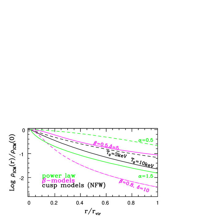
Figure 2.: The density profiles of hydrostatic equilibrium models described in section 3, in the isothermal case.

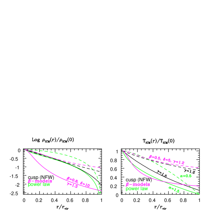
Figure 3.: The density and temperature profiles of hydrostatic equilibrium models described in section 3, in the polytropic case.

3.2. Results

We estimated $<Z_{\rm ICM}>_{L}/<Z_{\rm ICM}>$ by adopting the following parameter values:

1) for the abundance profile $b=0.2$, i.e., we considered a sort of “cuspy” profile, as observed in some clusters (e.g., De Grandi & Molendi 2001; Arnaud, this meeting), and $b=1$, a linear dependence on radius. The results are almost independent of $Z_{0}$.

2) the temperatures are $T_{0}=3$ and 10 keV in the isothermal case; these are central temperatures, in the polytropic case. This assumption encompasses the values observed for rich galaxy clusters (e.g., Markevitch et al. 1998).

3) $1<\gamma\leq 5/3$ in the polytropic case. This includes the $\gamma=1.2$ value that gives a “good” fit of some observed temperature profiles for ICM’s described by a $\beta$-model (Markevitch et al. 1998).

4) for the power law models $\alpha=0.5$ and 1.5.

5) for the $\beta$-models: $\beta=0.5$ and 0.8, $\delta=5$ and 10.

The general trend of the values derived for $<Z_{\rm ICM}>_{L}/<Z_{\rm ICM}>$ is that:

$\bullet$ $<Z_{\rm ICM}>_{L}/<Z_{\rm ICM}>$ always increases for centrally steeper abundance profiles (i.e., lower $b$ values) and steeper gas density profiles (i.e., higher $T_{0}$, $\alpha$, $\beta$ and $\delta$).

$\bullet$ $<Z_{\rm ICM}>_{L}/<Z_{\rm ICM}>$ is always $>1$, and it assumes the values below:

isothermal case                  polytropic case

a. NFW:                           1.4–1.7                                   1.4–1.7

b. POWER LAW:             1.3–1.8                                   1.3–1.5

c. $\beta$-MODELS:                 1.4–2.1                                   1.5–2.2

$\bullet$ The typical range of values for $<Z_{\rm ICM}>_{L}/<Z_{\rm ICM}>$ is 1.4–2, quite insensitive to variations of density and temperature profiles in the chosen (large) range.

4. Cooling flow models

We assume the ICM to be described by two gas phases, at two fixed temperatures $T_{\rm cool}$ and $T_{\rm amb}$, in pressure equilibrium within the cooling radius $r_{\rm cool}$. Outside $r_{\rm cool}$ there is only the ambient gas at $T_{\rm amb}$ (Ettori 2001). So:

$$\rho_{\rm ICM}(r)=\rho_{\rm 0,cool}\times\left[1-\left({r\over r_{\rm cool}}\right)^{2}\right]^{1.5{\beta_{\rm cool}}}+\rho_{\rm 0,amb}\times\left[1+\left({r\over{r_{c}}}\right)^{2}\right]^{-1.5{\beta_{\rm amb}}}.$$

Correspondingly the X-ray surface brightness profile is given by the superposition

$$\Sigma_{\rm X}(R)=\Sigma_{\rm X0,cool}\times\left[1-\left({R\over r_{\rm cool}}\right)^{2}\right]^{0.5+3\beta_{\rm cool}}+\Sigma_{\rm X0,amb}\times\left[1+\left({R\over r_{c}}\right)^{2}\right]^{0.5-3\beta_{\rm amb}}.$$

For two well studied cooling flow clusters, for which this decomposition has been made (Ettori 2001), we find $<Z_{\rm ICM}>_{L}/<Z_{\rm ICM}>$ as given in Table 1 (for $b=0.2$ and 1).

Table 1.: Results for cooling flow models

Cluster	$\delta$	$r_{c}=r_{\rm cool}$	$T_{\rm cool}$	$T_{\rm amb}$	$\beta_{\rm cool}$	$\beta_{\rm amb}$	$<Z_{\rm ICM}>_{L}/<Z_{\rm ICM}>$
		$(h_{50}^{-1}$Mpc)	(keV)	(keV)
A1795	5.8	0.26	0.5–1.1	7.4	1.801	0.761	1.6–2.0
A2199	11.5	0.13	0.4–0.8	4.6	1.635	0.644	1.7–2.1

5. Future developements

We plan to do the following further investigation:

1) Calibrate $<Z_{\rm ICM}>_{L}/<Z_{\rm ICM}>$ for axisymmetric and triaxial models (not significantly different results are expected).

2) Calibrate $<Z_{\rm ICM}>_{\rm depr}/<Z_{\rm ICM}>$ for axisymmetric and triaxial models, by considering their projection at different viewing angles, by circularizing and deprojecting their X-ray properties, by deriving putative 3-D $\rho_{\rm ICM}(r)$ and $Z_{\rm ICM}(r)$ and comparing $M^{\rm Z}_{\rm ICM,depr}=4\pi\int r^{2}\rho_{\rm ICM}(r)Z_{\rm ICM}(r)dr$ with the true value $M^{\rm Z}_{\rm ICM}$.

3) Evaluate $<Z_{\rm ICM}>_{L}/<Z_{\rm ICM}>$ for ICM’s resulting from high resolution numerical hydrodynamic simulations that include dark matter, gas and star formation (Cen & Ostriker 2000).

References

Cavaliere, A., Fusco-Femiano, R. 1976, A&A, 49, 137

Cen, R., Ostriker, J.P. 2000, ApJ, 538, 83

De Grandi, S., Molendi, S. 2001, ApJ, 551, 153

Ettori, S. 2000, MNRAS, 318, 1041

Ettori, S. 2001, preprint (astro-ph/0005224)

Evrard, A.E., Metzler, C.A., Navarro, J.F. 1996, ApJ, 469, 494

Finoguenov, A., Ponman, T.J. 1999, MNRAS, 305, 325

Finoguenov, A., David, L.P., Ponman, T.J. 2000, ApJ, 544, 188

Irwin, J.A., Bregman, J.N. 2001, ApJ, 546, 150

Jones, C., Forman, W. 1999, ApJ, 511, 65

Lloyd-Davies, E.J., Ponman, T.J., Cannon, D.B. 2000, MNRAS, 315, 689

Markevitch, M., Forman, W.R., Sarazin, C.L., Vikhlinin, A. 1998, ApJ, 503, 77

Mohr, J.J., Mathiesen, B., Evrard, E. 1999, ApJ517, 627

Navarro, J.F., Frenk, C.S., White, S.D.M. 1996, ApJ, 462, 563

Ponman, T.J., Cannon, D.B., Navarro, J.F. 1999, Nature, 397, 135

Renzini, A., Ciotti, L., D’Ercole, A., Pellegrini, S. 1993, ApJ, 419, 52

Wu, K.K.S., Fabian, A.C., & Nulsen, P.E.J. 2000, MNRAS, 318, 889

Xue, Y., Wu, X. 2000, ApJ, 538, 65