Effects of Foreground Contamination on the Cosmic Microwave Background Anisotropy Measured by MAP

Abstract

We study the effects of diffuse Galactic, far-infrared extragalactic source, and radio point source emission on the cosmic microwave background (CMB) anisotropy data anticipated from the MAP experiment. We focus on the correlation function and genus statistics measured from mock MAP foreground-contaminated CMB anisotropy maps generated in a spatially-flat cosmological constant dominated cosmological model.

Analyses of the simulated MAP data at 90 GHz ($0\hbox{$.\!\!^{\circ}$}3$ FWHM resolution smoothed) show that foreground effects on the correlation function are small compared with cosmic variance. However, the Galactic emission, even just from the region with $|b|>20^{\circ}$, significantly affects the topology of CMB anisotropy, causing a negative genus shift non-Gaussianity signal. Given the expected level of cosmic variance, this effect can be effectively reduced by subtracting existing Galactic foreground emission models from the observed data. IRAS and DIRBE far-infrared extragalactic sources have little effect on the CMB anisotropy. Radio point sources raise the amplitude of the correlation function considerably on scales below $0\hbox{$.\!\!^{\circ}$}5$, and also result in an asymmetry of the genus curve (at 2 $\sigma$) on $0\hbox{$.\!\!^{\circ}$}5$ scales. While the removal of bright sources above 5 $\sigma$ detection limit effectively reduces the excess correlation, the genus asymmetry remains significant. Accurate radio point source data is essential for an unambiguous detection of CMB anisotropy non-Gaussianity on these scales.

When all the foreground sources are subtracted from the observed CMB anisotropy map, non-Gaussianity of cosmological origin can be detected at the 2 $\sigma$ level if the measured genus shift parameter $|\Delta\nu|\gtrsim 0.02$ ($0.04$) or if the measured genus asymmetry parameter $|\Delta g|\gtrsim 0.03$ ($0.08$) on a $0\hbox{$.\!\!^{\circ}$}3$ ($1\hbox{$.\!\!^{\circ}$}0$) FWHM scale.

1 Introduction

Following the COBE-DMR experiment detection of anisotropy in the cosmic microwave background (CMB) on large angular scales (Bennett et al. 1996; Górski et al. 1996, 1998), there have been many measurements of CMB anisotropy on angular scales down to $\sim 10^{\prime}$ (see, e.g., Lee et al. 2001; Netterfield et al. 2001; Halverson et al. 2001 for recent measurements of CMB anisotropy). These observations have begun to test cosmological models and provide interesting constraints on cosmological parameters (see, e.g., Kamionkowski & Kosowsky 1999; Rocha 1999; Gawiser & Silk 2000 for reviews, and, e.g., Ratra et al. 1999a, 1999b; Rocha et al. 1999; Knox & Page 2000; Wang & Mathews 2000; Douspis et al. 2001; Podariu et al. 2001; Xu, Tegmark, & de Oliveira-Costa 2001; Netterfield et al. 2001; Pryke et al. 2001; Stompor et al. 2001 for CMB anisotropy tests and constraints).

A satellite mission, the Microwave Anisotropy Probe (MAP), will probe the CMB anisotropy at frequencies of 22, 30, 40, 60, and 90 GHz with expected angular resolutions of $0\hbox{$.\!\!^{\circ}$}93$, $0\hbox{$.\!\!^{\circ}$}68$, $0\hbox{$.\!\!^{\circ}$}47$, $0\hbox{$.\!\!^{\circ}$}35$, and $0\hbox{$.\!\!^{\circ}$}21$ FWHM, respectively. At 90 GHz the sensitivity of MAP is expected to be $\sim 35$ $\mu\rm K$ per $0\hbox{$.\!\!^{\circ}$}3\times 0\hbox{$.\!\!^{\circ}$}3$ pixel. The high quality CMB anisotropy data anticipated from MAP will significantly improve constraints on many cosmological parameters.

Non-CMB foreground contamination must be understood and accounted for to fully utilize the cosmological discriminative power of MAP CMB anisotropy data. Recent rapid progress in the CMB anisotropy field has stimulated much work on modeling foregrounds and on developing methods for removing them from acquired data (see, e.g., Bennett et al. 1992, 1994; Brandt et al. 1994; Dodelson & Stebbins 1994; Tegmark & Efstathiou 1996; Bouchet & Gispert 1999; Tegmark et al. 2000). There are two major potential sources for foreground contamination: diffuse Galactic emission and unresolved point sources.

Kogut et al. (1996a, 1996b, hereafter K96) detect cross-correlations between the COBE-DMR and DIRBE maps, which they ascribe to Galactic dust and free-free emission. Using the Saskatoon data ($\sim$ 30 to 40 GHz, $\sim 1^{\circ}$ resolution, Netterfield et al. 1997) and the 19 GHz survey data ($\sim 3^{\circ}$ resolution, Boughn et al. 1992), de Oliveira-Costa et al. (1997, 1998) obtain a result similar to that of Kogut et al. Hamilton & Ganga (2001) find similar correlations using the UCSB South Pole 1994 data ($\sim$ 30 to 40 GHz, $\sim 1^{\circ}$ resolution, Gundersen et al. 1995; Ganga et al. 1997). At higher frequencies near 100 GHz and on similar angular scales, MAX data (Lim et al. 1996; Ganga et al. 1998) shows a similar correlation. On smaller angular scales Leitch et al. (2000) reach a similar conclusion using the OVRO data ($\sim$ 30 GHz). However, no such correlation is found in the Python V data ($\sim$ 40 GHz, $\sim 1^{\circ}$ resolution, Coble et al. 1999). Mukherjee et al. (2001) and de Oliveira-Costa et al. (2000) discuss foreground contamination of the lower frequency, larger scale Tenerife data. At frequencies higher than 60 GHz there is no significant correlation between CMB maps and various synchrotron template maps such as the 408 MHz (Haslam et al. 1981) and the 1420 MHz (Reich & Reich 1988) radio survey maps (Kogut et al. 1996a; K96; de Oliveira-Costa et al. 1997, 1998).

CMB anisotropy experiments with subdegree resolution may be sensitive to radio point sources. Gawiser & Smoot (1997) study the effect of far-infrared (FIR) point source contamination of CMB anisotropy data by using the IRAS 1.2 Jy flux-limited galaxy catalog at various angular resolutions and observation frequencies. Gawiser, Jaffe, & Silk (1998a) derive upper and lower limits on microwave anisotropy from point sources over the range of frequencies 10 to 1000 GHz from recent sub-arcminute resolution point source observations. Their upper limit is $\langle(\Delta T/T)^{2}\rangle^{1/2}\sim 10^{-5}$ for a $10^{\prime}$ beam at 100 GHz. Toffolatti et al. (1998) use a luminosity evolution model to make predictions for the number density distribution of extragalactic sources and their contribution to temperature fluctuations in each channel of the Planck Surveyor mission. Sokasian, Gawiser, & Smoot (1998) estimate the effect of bright radio point source contamination on MAP and Planck observations. They find that removing bright sources above the source detection limit (5 $\sigma\simeq 1$ Jy, where $\sigma$ is the rms level of CMB anisotropy measured) reduces the contamination from $\langle(\Delta T/T)^{2}\rangle^{1/2}\sim 10^{-5}$ to $10^{-6}$, consistent with the conclusion of Toffolatti et al. (1998). Recently, the Wavelength-Oriented Microwave Background Analysis Team (WOMBAT, Gawiser et al. 1998b; Jaffe et al. 1999) have presented many different all-sky high resolution CMB anisotropy contaminant foreground template maps, including those for Galactic dust, synchrotron, FIR point source, radio point source, and Sunyaev-Zel’dovich cluster emission.

In this paper we generate mock all-sky foreground-contaminated CMB anisotropy maps for the 90 GHz channel of MAP in a spatially-flat cosmological constant ($\Lambda$) dominated cold dark matter (CDM) cosmogony. We use these maps to investigate how foreground contamination affects the CMB anisotropy angular correlation function $C(\theta)$ and the topology of CMB anisotropy. In $\S$2 we summarize various foreground contamination sources. In $\S$3 we summarize how mock foreground-contaminated CMB anisotropy maps are generated. In $\S$4 we study the effects of foreground contamination on the amplitude and shape of the correlation function, focussing particularly on the location of the acoustic valley in the function $\theta^{1/2}C(\theta)$. In $\S$5 we use the genus statistic to study the effect of foreground contamination on detecting non-Gaussianity of cosmological origin in the $MAP$ data. We conclude in $\S$6.

2 Sources of Foreground Contamination

2.1 Galactic Dust and Free-Free Emissions

In the microwave sky three Galactic emission components, those due to synchrotron, free-free, and dust, are important. Although these Galactic foregrounds can be modeled theoretically pixel by pixel by multifrequency observations (Brandt et al. 1994), this requires very low instrument noise and accurate emission models. According to Bennett et al. (1992), synchrotron and free-free emissions have well-determined spectral behaviors with $I_{\nu}\propto\nu^{-0.7\sim-1.1}$ and $I_{\nu}\propto\nu^{-0.15}$, respectively. It is very difficult to produce an accurate all-sky dust emission model because its spectral behavior depends on the shape, composition, size distribution, and dynamics of the dust grains, and because the dust emission is a sum over the emission from all dust grains along each line of sight.

Kogut et al. (1996a) and K96 apply a constant temperature warm dust and free-free emission model with spectral intensity

$$I_{\nu}=\tau(\nu/\nu_{0})^{\beta}B_{\nu}(T)+A_{ff}(\nu/\nu_{0})^{-0.15}$$

to the DIRBE maps and the DMR two- and four-year data. Here $B_{\nu}(T)$ is the Planck black body function, $\tau$ opacity, $\beta$ emissivity power-law index, $\nu_{0}=900$ GHz, and $A_{ff}$ the normalized amplitude of free-free emission. For the four-year DMR data they obtain $\tau=(1.2_{-0.4}^{+0.7})\times 10^{-5}$, $T=20.0_{-4.0}^{+2.5}$ K, and $\beta=1.5_{-0.3}^{+1.1}$ (68% confidence limits) at $|b|>20^{\circ}$. In eq. (1) the second term represents free-free emission, where the constant $A_{ff}$ is determined from the rms level of DMR-DIRBE correlated free-free emission, $\Delta T_{ff}=7.1\pm 1.7$ $\mu$K at 53 GHz (see $\S$3 of K96). Since synchrotron emission is dominant only at frequencies lower than about 60 GHz, we neglect synchrotron emission in our analyses here. Figure 1 shows the spectra of the dust plus free-free emission model of K96. The thick solid curve represents the best-fit model. The upper and lower thin solid curves are the upper ($T=22.5$ K, $\beta=1.2$) and lower ($T=16.0$ K, $\beta=2.6$) limits of the K96 model. $\tau=1.2\times 10^{-5}$ in all three cases. The dust temperature is almost inversely proportional to the emissivity (Kogut et al. 1996a).

However, dust emission models with a constant dust temperature everywhere on the sky are a poor description of reality (e.g., Finkbeiner, Davis, & Schlegel 1999, hereafter FDS99). It is known from FIRAS observations that there seem to exist both warm ($16$ K $<T<21$ K) and cold ($4$ K $<T<7$ K) dust components that contribute to Galactic dust emission (Wright et al. 1991; Reach et al. 1995). FDS99 provide a two-component temperature-varying dust model determined by fitting 100 $\mu$m dust emission data (Schlegel, Finkbeiner, & Davis 1998, described below) to FIRAS dust spectra. Their model parameter values are $\alpha_{1}=1.67$, $\alpha_{2}=2.70$, $f_{1}=0.0363$, and $q_{1}/q_{2}=13.0$, where $\alpha_{i}$ is the $i^{\rm th}$ dust component emissivity index, $f_{i}$ is the fraction of power absorbed and re-emitted by dust component $i$ (with $\sum_{k}f_{k}=1$), and $q_{i}$ is the ratio of the FIR emission cross-section to the UV/optical absorption cross-section for the $i^{\rm th}$ component (see FDS99 $\S$4 for details). We use both the K96 one-component and the FDS99 two-component dust models in our analyses here.

We need a high resolution Galactic emission map to model foreground contamination in the 90 GHz MAP CMB anisotropy data. Schlegel et al. (1998) present a well-calibrated and Fourier-destriped full-sky 100 $\mu{\rm m}$ Galactic emission map constructed from the COBE-DIRBE and IRAS-ISSA data sets, with zodiacal light and point source contamination removed. This map has an angular resolution of $6\hbox{$.\mkern-4.0mu^{\prime}$}1$ FWHM. We smooth this map using a Gaussian filter to get a map with total smoothing scale of $0\hbox{$.\!\!^{\circ}$}21$ FWHM, and estimate the brightness temperature at 90 GHz by using the Galactic emission spectrum template shown in Figure 1. For the FDS99 two-component dust model we estimate the 90 GHz dust emission by extrapolating the 100 $\mu$m flux using the dust temperature and DIRBE color-correction factor for each line of sight in the maps (see eq. [6] in $\S$4 of FDS99). The averaged FDS99 dust emission spectrum (the thick long-dashed curve in Fig. 1) is a factor of 1.4 lower than that of the K96 dust model. Since the FDS99 model does not include free-free emission, we generate a Galactic emission contamination map by adding free-free emission, assumed to be proportional to dust emission and to have an amplitude equal to 18% of the dust emission amplitude at 90 GHz, which is the percentage of the excess dust-correlated DMR emission estimated by FDS99 (see Table 4 of FDS99). Thermodynamic temperature fluctuations with respect to the mean CMB temperature $T_{0}=2.728$ K (Fixsen et al. 1996) can be obtained from brightness temperature fluctuations multipied by the Planck factor $(e^{x}-1)^{2}/x^{2}e^{x}$, where $x=h\nu/kT_{0}$. This results in a high resolution all-sky temperature fluctuation map for Galactic emission that contributes to the MAP 90 GHz band data.

While this is the best available map, it is not ideal. First, the K96 model parameters are determined from large (DMR) angular scale data while we study small-scale microwave temperature fluctuations. Second, the ratio of free-free to dust emission may be position dependent, resulting in a position-dependent $A_{ff}$ (while we assume that $A_{ff}$ is a constant). Third, if the free-free emission power spectrum is flatter than the dust emission power spectrum $P(\ell)\propto\ell^{-3}$ in multipole space, the ratio of free-free to dust emission will increase with decreasing angular scale (we assume that the large scale dust emission correlation with free-free emission persists to smaller scales).

In this paper we use the K96 model free-free emission term to account for about 20% of the dust-correlated emission (see FDS99 for a related discussion). Similar correlations have been detected for many CMB observations (see $\S$1, and Kogut 1999 for a review). This excess microwave emission is clearly correlated with the dust but is not due to thermal (vibrational) dust emission. Draine & Lazarian (1998) propose that K96’s dust-correlated emission is not free-free emission but emission from rapidly spinning dust grains. Nevertheless, even if the dust-correlated emission is not free-free emission, our phenomenological approach is fairly reasonable, especially at 90 GHz.

2.2 Far Infrared Extragalactic Sources

The IRAS 1.2 Jy flux-limited galaxy catalog (Strauss et al. 1990; Fisher et al. 1995) contains 5,319 galaxies, almost all of which are inactive spiral galaxies though some are active star-forming galaxies and active galactic nuclei. The IR emission from inactive spiral galaxies is from reradiation of interstellar dust heated by the general interstellar radiation field (Helou 1986). Assuming that these IRAS galaxies are all inactive spirals with emission spectrum similar to that of our Galaxy, we transform their 100 $\mu{\rm m}$ fluxes to 90 GHz by using the K96 Galactic emission spectrum. We also use the method of Gawiser & Smoot (1997) and Gawiser et al. (1998a) to determine the rms thermodynamic temperature fluctuation caused by IRAS extragalactic sources, and obtain $\langle(\Delta T/T)^{2}\rangle^{1/2}\simeq 5\times 10^{-7}$ at 90 GHz and $0\hbox{$.\!\!^{\circ}$}21$ FWHM angular resolution. This is consistent with the result of Gawiser & Smoot (1997).

A second set of contaminating FIR extragalactic sources are the few hundred sources we have tentatively detected in the DIRBE maps. DIRBE observed the whole sky with a $0\hbox{$.\!\!^{\circ}$}7\times 0\hbox{$.\!\!^{\circ}$}7$ square beam and produced infrared maps at 10 near-to-far infrared wavelengths, with pixel size of $0\hbox{$.\!\!^{\circ}$}32\times 0\hbox{$.\!\!^{\circ}$}32$. We use the ZSMA (Zodiacal light-Subtracted Mission Average) maps at 12, 25, 60, 100, 140, and 240 $\mu{\rm m}$ to search for dim signals in the maps. We generate a difference map at each band by subtracting the intensity map smoothed over $2\hbox{$.\!\!^{\circ}$}36$ FWHM from the original unsmoothed map. Thus only signals on scales smaller than $2\hbox{$.\!\!^{\circ}$}36$ remain in the difference maps. The $i^{\rm th}$ pixel noise $\sigma_{i}$ in the difference map is $\sigma_{i}=\sigma_{N}/\sqrt{N_{i}}$, where $\sigma_{N}$ is the global noise level of the difference map and $N_{i}$ is the number of observations at the $i^{\rm th}$ pixel. $\sigma_{N}$ can be determined iteratively from the less-contaminated background region ($|b|>60^{\circ}$ and ecliptic latitude $|\beta|>20^{\circ}$) by requiring $z=I_{i}/\sigma_{i}$ (where $I_{i}$ is the intensity at $i^{\rm th}$ pixel) to have a normal distribution with zero mean and unit variance at $z<0$. The resulting global noise levels are 0.209, 0.295, 0.549, 1.14, and 34.8, and 19.9 MJy/sr at 12, 25, 60, 100, 140, and 240 $\mu{\rm m}$, respectively. The noise levels in the 140 and 240 $\mu{\rm m}$ difference maps are very large so we exclude these maps from our analysis.

In the region $|b|>20^{\circ}$ of the 100 $\mu{\rm m}$ map we select pixels with $I_{i,100~{}\mu{\rm m}}>3\sigma_{i}$. A faint extragalactic source may appear in at most 4 pixels ($0\hbox{$.\!\!^{\circ}$}64\times 0\hbox{$.\!\!^{\circ}$}64$) in the DIRBE map, when it is located where the 4 pixels touch. By grouping contiguous pixels, we search for signals in groups of 4 or fewer pixels in the Quadrilateralized Spherical Cube projection (see COBE DIRBE Exp. Supp. 1998). This excludes most of the bright galaxies detected by Odenwald, Newmark, & Smoot (1998), since they are typically detected in more than 4 pixels. We find 421 and 401 such groups (with 4 or fewer pixels) in the Galactic north and south hemispheres, respectively. 436 of these groups have positive fluxes at all wavelengths considered. We finally catalogue 289 extragalactic source candidates satisfying the IRAS bright galaxy color criteria (Smith et al. 1987; Soifer et al. 1989; Strauss et al. 1990). These color criteria are $-0.9<\log(f_{60~{}\mu{\rm m}}/f_{100~{}\mu{\rm m}})<0.3$, $-1.5<\log(f_{25~{}\mu{\rm m}}/f_{60~{}\mu{\rm m}})<0.0$, $-1.2<\log(f_{12~{}\mu{\rm m}}/f_{25~{}\mu{\rm m}})<0.4$, $-2.1<\log(f_{12~{}\mu{\rm m}}/f_{60~{}\mu{\rm m}})<0.0$, and $f_{60~{}\mu{\rm m}}^{2}>f_{12~{}\mu{\rm m}}f_{25~{}\mu{\rm m}}$. Figure 2 shows the distribution of the final 289 DIRBE FIR sources. 33 IRAS galaxies and only one source in the 5 GHz 1 Jy flux-limited extragalactic radio source catalog (518 objects, Kühr et al. 1981) are within a radius of $0\hbox{$.\!\!^{\circ}$}32$ of these DIRBE sources. Most of these sources are matched with extragalactic objects in the IRAS Faint Source Catalog within the same radius. However, the large DIRBE pixel size prevents us from uniquely identifying these sources as extragalactic because each DIRBE pixel contains many IRAS sources, some of which are not extragalactic. Some of the DIRBE sources could conceivably be objects in our Galaxy that coincidentally satisfy the IRAS galaxy color criteria. The emission from these DIRBE FIR sources (after exclusion of the 33 sources identified with IRAS galaxies) are transformed to 90 GHz thermodynamic temperature fluctuations using the method applied above to the IRAS galaxies.

2.3 Radio Point Sources

The 4.85 GHz Green Bank survey catalog (Becker, White, & Edwards 1991) contains 53,522 radio point sources with fluxes larger than about 40 mJy and covers $0^{\circ}<\delta<75^{\circ}$. The 4.85 GHz Parkes-MIT-NRAO survey catalog (Griffith & Wright 1993) has 50,814 point sources with a flux limit of about 35 mJy in the $-87\hbox{$.\!\!^{\circ}$}5<\delta<10^{\circ}$ region. Besides these, there is a 1.4 GHz survey catalog that has 30,239 sources flux-limited at 100 mJy in the $-5^{\circ}<\delta<82^{\circ}$ region (White & Becker 1992). These catalogs contain extragalactic sources as well as Galactic radio sources. For example, the Green Bank survey catalog has about 350 galaxies, $\sim 800$ quasars, more than 500 BL Lacertae objects, and $\sim 400$ X-ray sources (Becker et al. 1991).

To make a combined radio source catalog that almost covers the sky, we adopt the Green Bank catalog for $0^{\circ}<\delta<75^{\circ}$, the Parkes-MIT-NRAO catalog for $-87\hbox{$.\!\!^{\circ}$}5\leq\delta\leq 0^{\circ}$, and the 1.4 GHz radio source catalog for $75^{\circ}<\delta<82^{\circ}$. In the few GHz frequency band, the main emission mechanism for radio sources is synchrotron radiation with power-law spectral behavior $I_{\nu}\sim\nu^{\alpha}$ with $-1.0\lesssim\alpha\lesssim-0.5$ (Platania et al. 1998). Since spectral indices of most sources in the Green Bank and Parkes-MIT-NRAO catalogs are close to $-0.85$, radio sources with unknown $\alpha$ are assumed to have $\alpha=-0.85$. Some radio sources with compact active nuclei generate flat-spectrum radio emission ($\alpha\geq 0$) due to self-absorption of low energy photons. The average spectral index of flat-spectrum compact sources is $\alpha\simeq 0$ at $\nu\leq 200$ GHz, steepening to $\alpha=-0.7$ at higher frequencies (Danese et al. 1987; Toffolatti et al. 1998). In our analyses here we set $\alpha=0$ for all radio sources with spectral index $\alpha>0$. Emission from radio sources in the region $75^{\circ}<\delta<82^{\circ}$ are transformed to 4.85 GHz fluxes using the spectral index determined above. The fluxes of the final 72,132 4.85 GHz sources, covering $-87\hbox{$.\!\!^{\circ}$}5<\delta<82^{\circ}$, with flux limit of 43 mJy, are converted to temperature fluctuations when “observed” with the $0\hbox{$.\!\!^{\circ}$}21$ FWHM MAP beam at 90 GHz.

3 Generating Mock MAP Maps

Park et al. (1998, hereafter P98) generate mock CMB anisotropy maps for the 90 GHz ($0\hbox{$.\!\!^{\circ}$}21$ FWHM beamwidth) channel of the MAP experiment in a spatially-flat $\Lambda$ dominated CDM model. This $\Lambda$CDM cosmogony has non-relativistic matter density parameter $\Omega_{0}=0.4$, $h=0.6$ (where the Hubble constant $H_{0}=100h$ km s^-1 Mpc^-1), baryonic-matter density parameter $\Omega_{B}=0.0125h^{-2}$, and is normalized to the four-year DMR data (Ratra et al. 1997). The rms level of the CMB anisotropy in this map is 104 $\mu{\rm K}$ (at $0\hbox{$.\!\!^{\circ}$}21$ FWHM), larger than that of the flat CDM case (92 $\mu{\rm K}$; Refregier, Spergel, & Herbig 2000). The maps include MAP instrumental noise, simulated to give 35 $\mu{\rm K}$ per $0\hbox{$.\!\!^{\circ}$}3\times 0\hbox{$.\!\!^{\circ}$}3$ pixel.

It is expected that MAP will produce CMB temperature fluctuation maps with zero mean even if foreground contamination is not completely removed. Thus in the map the observed temperature at each position on the sky, $T(\theta,\phi)$, is the sum of the CMB contribution $T_{0}+\delta T_{CMB}$, a contribution from foreground contamination $\delta T_{C}$, and an instrumental noise contribution $\delta T_{N}$, where $T_{0}$ is CMB black body temperature (2.728 K) and $\delta T_{CMB}$ is the CMB anisotropy temperature. Therefore the observed temperature anisotropy is

$${{\delta T}\over{T}}(\theta,\phi)\equiv{{T(\theta,\phi)-\langle T\rangle}\over{\langle T\rangle}}\simeq{{\delta T_{CMB}(\theta,\phi)+\delta T_{C}(\theta,\phi)+\delta T_{N}(\theta,\phi)-\langle\delta T_{C}\rangle}\over{T_{0}}}$$

where $\langle\cdots\rangle$ represents an average over the whole sky excluding the Galactic plane region (typically the $|b|>20^{\circ}$ part of the sky in our analyses here), and $\langle\delta T_{CMB}\rangle=\langle\delta T_{N}\rangle=0$ are assumed. The term $\langle\delta T_{C}\rangle$ that will appear in the denominator of the last expression is omitted, since it is negligible compared with $T_{0}$.

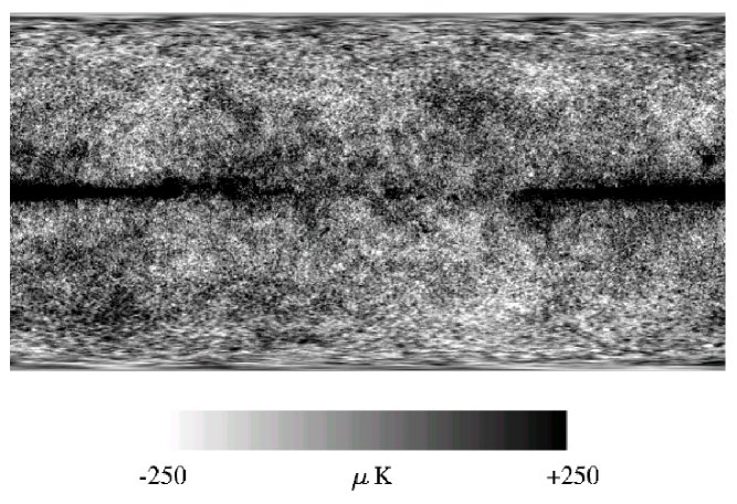
Figure 3: The $\Lambda$CDM model foreground-contaminated CMB anisotropy temperature fluctuation mock map for the 90 GHz MAP channel, smoothed to $0\hbox{$.\!\!^{\circ}$}3$ FWHM angular resolution. Foreground contamination here is modelled by the K96 Galactic emission model.

We use eq. (2) to generate foreground-contaminated CMB temperature fluctuation maps at 90 GHz with $0\hbox{$.\!\!^{\circ}$}21$ FWHM resolution. These maps are further smoothed over $0\hbox{$.\!\!^{\circ}$}214$ (i.e., a total smoothing scale of $0\hbox{$.\!\!^{\circ}$}3$ FWHM) to reduce noise, and consist of $3600\times 1801$ points in $(\ell,b)$ space with $0\hbox{$.\!\!^{\circ}$}1$ spacing. Figure 3 shows one of the foreground-contaminated CMB temperature fluctuation maps (using the K96 Galactic emission model). The Galactic emission model has an uncertainty. Its uncertainty (hereafter $\Delta$G) is taken to be the difference between the maps generated from the K96 (constant dust temperature) and FDS99 (spatially-varying dust temperature) Galactic emission models. Table 1 lists the map rms values of the CMB temperature fluctuations, MAP instrumental noise, and various foreground emissions. Note that rejecting radio sources above 5 $\sigma$ reduces the rms level of temperature fluctuations. When analyzing the maps we mask the LMC, SMC, M31 and Orion-Taurus regions for Galactic emission-contaminated maps. For radio source emission-contaminated maps we mask regions that are not surveyed ($\delta>82^{\circ}$, $\delta<-87.5^{\circ}$) or only partially surveyed.

4 Correlation Function

4.1 Amplitude of Correlation Function

The two-point angular correlation function (hereafter CF) for temperature anisotropy is $C(\theta)\equiv\langle\delta T/T(\theta_{i},\phi_{i})\delta T/T(\theta_{j},\phi_{j})\rangle$, where $\langle\cdots\rangle$ denotes an ensemble average and $\theta$ is the angular separation between $(\theta_{i},\phi_{i})$ and $(\theta_{j},\phi_{j})$. It is related to the angular power spectrum $C_{\ell}$ through

$$C(\theta)=\sum_{\ell=2}^{\infty}{{2\ell+1}\over{4\pi}}C_{\ell}P_{\ell}(\cos\theta)B_{\ell}^{2}F_{\ell}^{2},$$

where $P_{\ell}$ is a Legendre polynomial and $B_{\ell}$ and $F_{\ell}$ are the coefficients of the beam function and smoothing filter expanded in a Legendre polynomial basis.

We measure $C(\theta)$ directly from the CMB maps by picking up a million pairs of points for each angular bin considered. Figure 4$a$ shows the angular CFs of noise-free and noise-added $\Lambda$CDM CMB anisotropy maps. The theoretical CMB anisotropy CF of the $\Lambda$CDM cosmological model (dot-dashed line) is also shown for comparison. Note that the amplitude of the CF can exhibit large cosmic variance while the position of the acoustic valley does not (see $\S$3 of P98 for the effect of cosmic variance on the position of the acoustic valley of the CF). The amplitude of the CF of the noise-added CMB map is slightly higher than that of the noise-free case on scales less than $0\hbox{$.\!\!^{\circ}$}3$. The effect of noise on the CF amplitude exceeds that of cosmic variance on these scales. On scales larger than $0\hbox{$.\!\!^{\circ}$}3$, however, instrumental noise hardly affects the CF and cosmic variance dominates the statistical uncertainty. The effect on the CF of Galactic plane cuts at $|b|=20^{\circ}$ and $40^{\circ}$ is illustrated in Figure 4$b$.

The effects of foreground emission on the CF are shown in Figure 5, where the CFs are computed for the Galactic plane cut region with $|b|>20^{\circ}$. Although foreground Galactic emission, modeled either by K96 or FDS99, slightly increases the correlation amplitude on all angular scales (Fig. 5$a$), these effects are smaller than the cosmic and sample variance uncertainties. Figure 5$b$ demonstrates that the Galactic emission model uncertainty $\Delta$G (i.e., Galactic emission residuals which remain after removing model Galactic emission from a foreground-contaminated map) hardly affects the CF. IRAS and DIRBE FIR extragalactic sources appear not to have any effect (Fig. 5$c$). Radio point source emission raises the CF amplitude on scales smaller than $0\hbox{$.\!\!^{\circ}$}5$. When bright radio sources above 5 $\sigma$ are removed this small-scale effect becomes much weaker (Fig. 5$d$).

4.2 Position of the Acoustic Valley

The Doppler peaks in the angular power spectrum, particularly the first Doppler peak, appear as an acoustic valley in $\theta^{1/2}C(\theta)$. The position, depth, and width of the acoustic valley depend on the cosmological model parameters (P98). In addition to the effect of foreground contamination on the amplitude of the CF, it is necessary to study their effect on the position of the acoustic valley.

To predict acoustic valley positions we compute $C(\theta)$ (using eq. [3]) from 200 sets of $a_{\ell}^{m}B_{\ell}$ and $(a_{\ell}^{m}B_{\ell}+n)F_{\ell}$ up to $\ell=2500$. We assume the noise $n$ is a Gaussian random variable with zero mean and variance appropriate for MAP, and here $B_{\ell}$ and $F_{\ell}$ represent the $0\hbox{$.\!\!^{\circ}$}21$ FWHM beam and $0\hbox{$.\!\!^{\circ}$}214$ FWHM smoothing filter, respectively. The uncertainty in the position of the acoustic valley was estimated from these 200 Monte Carlo realizations (P98). The $\Lambda$CDM model predicts the location of the acoustic valley to be at $\theta_{\rm v}=1\hbox{$.\!\!^{\circ}$}12\pm 0\hbox{$.\!\!^{\circ}$}02$ for a $0\hbox{$.\!\!^{\circ}$}21$ beam. When we account for the MAP noise and use an additional $0\hbox{$.\!\!^{\circ}$}214$ FWHM smoothing filter (total smoothing of $0\hbox{$.\!\!^{\circ}$}3$ FWHM), the position becomes $\theta_{\rm v}=1\hbox{$.\!\!^{\circ}$}14\pm 0\hbox{$.\!\!^{\circ}$}02$ while it is $0\hbox{$.\!\!^{\circ}$}65\pm 0\hbox{$.\!\!^{\circ}$}04$ for an open CDM model with $\Omega_{0}=0.4$, $h=0.65$.

We have also computed $C(\theta)$ near the acoustic valley directly from the foreground-contaminated CMB anisotropy maps, and have measured the position of the acoustic valley. The results are shown in Figure 6 and Table 2. The location of the acoustic valley is quite robust. When foreground Galactic emission is reasonably modeled, the Galactic cut mainly affects its location ($\sim 0\hbox{$.\!\!^{\circ}$}01$). The cosmic variance is about $0\hbox{$.\!\!^{\circ}$}02$.

5 Topology

5.1 The Genus

Gaussianity and phase correlation information are important probes of the origin of structure formation. Topology measures for two-dimensional fields, first introduced by Coles & Barrow (1987), Melott et al. (1989) and Gott et al. (1990), have been applied to observational data such as the angular distribution of galaxies on the sky (Coles & Plionis 1991; Gott et al. 1992), the distribution of galaxies in slices of the universe (Park et al. 1992; Colley 1997; Park, Gott, & Choi 2001a), and the CMB temperature fluctuation field (Coles 1988; Gott et al. 1990; Smoot et al. 1994; Kogut et al. 1996c; Colley, Gott, & Park 1996; Park et al. 2001b).

We use the two-dimensional genus statistic introduced by Gott et al. (1990) as a quantitative measure of the topology of the CMB anisotropy. For the CMB the genus is the number of hot spots minus the number of cold spots. Equivalently, the genus at a temperature threshold level $\nu$ is

$$g(\nu)={1\over 2\pi}\int_{C}\kappa ds,$$

where $\kappa$ is the signed curvature of the iso-temperature contours $C$, and the threshold level $\nu$ is the number of standard deviations from the mean. At a given threshold level, we measure the genus by integrating the curvature along iso-temperature contours. The curvature is positive (negative) if the interior of a contour has higher (lower) temperature than the specified threshold level.

The genus of a two-dimensional random-phase Gaussian field is $g(\nu)\propto\nu e^{-\nu^{2}/2}$ (Gott et al. 1990). Non-Gaussian features in the CMB anisotropy will appear as deviations of the genus curve from this relation (P98; Park et al. 2001a, 2001b). Non-Gaussianity can shift the observed genus curve to the left (toward negative thresholds) or right near the mean threshold level. The shift $\Delta\nu$ of the genus curve with respect to the Gaussian relation is measured by minimizing the $\chi^{2}$ between the data and the fitting function

$$G=A_{s}\nu^{\prime}e^{-{\nu^{\prime}}^{2}/2},$$

where $\nu^{\prime}=\nu-\Delta\nu$, and the fitting is performed over the range $-1.0\leq\nu\leq 1.0$. Non-Gaussianity can also alter the amplitudes of the genus curve at positive and negative levels differently causing $|g(\nu\approx-1)|\neq|g(\nu\approx+1)|$. The asymmetry parameter is defined as

$$\Delta g=A_{H}-A_{C},$$

where

$$A_{H}=\int_{\nu_{1}}^{\nu_{2}}g_{\rm obs}d\nu/\int_{\nu_{1}}^{\nu_{2}}g_{\rm fit}d\nu,$$

and likewise for $A_{C}$. The integration is limited to $-2.4\leq\nu\leq-0.4$ for $A_{C}$ and to $0.4\leq\nu\leq 2.4$ for $A_{H}$. The overall amplitude $A$ of the best-fit Gaussian genus curve $g_{\rm fit}$ is found from $\chi^{2}$-fitting over the range $-2.4\leq\nu\leq 2.4$. Positive $\Delta g$ means that more hot spots are present than cold spots. This kind of topological information can not be drawn simply from the one-point distribution. In summary, for a given genus curve we measure the best-fit amplitude $A$, the shift parameter $\Delta\nu$, and the asymmetry parameter $\Delta g$.

5.2 Effects of Foregrounds on CMB Anisotropy Topology

We use our mock foreground-contaminated CMB anisotropy maps for the MAP experiment to study the sensitivity of the genus statistic to non-Gaussianity of cosmological origin. To compute the genus we stereographically project the maps on to a plane. This conformal mapping locally preserves shapes of structures. Additional Gaussian smoothings are applied during the projection so that the projected maps have total smoothing scales of $0\hbox{$.\!\!^{\circ}$}3$, $0\hbox{$.\!\!^{\circ}$}5$ and $1\hbox{$.\!\!^{\circ}$}0$ FWHM. We then exclude regions with $|b|<20^{\circ}$ to reduce the effect of Galactic emission. We present the genus curves as a function of the area fraction threshold level $\nu_{A}$, which is defined to be the temperature threshold level at which the corresponding iso-temperature contour encloses a fraction of the survey area equal to that at the temperature threshold level $\nu_{A}$ for a Gaussian field (Gott et al. 1990). The $\nu_{A}=0$ level corresponds to the median temperature because this threshold level divides the map into high and low regions of equal area. All our analyses are based on genus curves measured as a function of $\nu_{A}$.

Figure 7 shows genus curves measured from the mock MAP CMB maps in the $\Lambda$CDM model with various foreground contaminations at $0\hbox{$.\!\!^{\circ}$}3$ FWHM resolution (open symbols). The genus curve of the foreground-free map (noise-added; filled circles) is shown for comparison. The effect of instrumental noise on the genus is significant on both $0\hbox{$.\!\!^{\circ}$}3$ and $0\hbox{$.\!\!^{\circ}$}5$ scales (filled circles in Fig. 7$a$; also see the genus amplitude parameter $A$ values in Table 3 described below). It should also be noted that the $0\hbox{$.\!\!^{\circ}$}3$ scale genus is reduced by the finite pixel size of the MAP simulation (Melott et al. 1989).

Table 3 lists the genus-related statistics $A$, $\Delta\nu$, and $\Delta g$ measured from CMB maps with $0\hbox{$.\!\!^{\circ}$}3$, $0\hbox{$.\!\!^{\circ}$}5$, and $1\hbox{$.\!\!^{\circ}$}0$ FWHM resolutions using eqs. (5) to (7). The uncertainties are $1\sigma$ errors derived from the variances over the eight octants and account for cosmic variance. Here $\Delta\nu_{0}$ and $\Delta g_{0}$ are the values from the noise- and foreground-free pure CMB anisotropy maps. Hence $\Delta\nu-\Delta\nu_{0}$ and $\Delta g-\Delta g_{0}$ are the net effects due to instrumental noise or foreground emission. Table 3 shows that Galactic emission significantly affects the shift parameter on all angular scales, at a level exceeding 2 $\sigma$. However, their effect become much less serious when only the Galactic emission model uncertainty $\Delta$G needs to be accounted for. FIR extragalactic source emission has minimal effect on the genus, on all angular scales. Radio point source emission results in positive genus asymmetry, particularly on intermediate angular scales ($0\hbox{$.\!\!^{\circ}$}5$ FWHM) at a statistical significance level of about 2 $\sigma$. We have also measured the genus from the radio source-contaminated CMB anisotropy map with $0\hbox{$.\!\!^{\circ}$}5$ FWHM resolution after broadly excising pixels above 4.7 times the rms level of the noise-added CMB anisotropy map, and find the asymmetry still exceeds cosmic variance ($\Delta g-\Delta g_{0}=0.035\pm 0.020$).

When Galactic diffuse emission and bright radio point source emission are removed from the observed temperature fluctuation map using accurate foreground models, one may conclude that non-Gaussianity of cosmological origin is present if the measured genus-related parameters $|\Delta\nu|\gtrsim 0.02$ ($0.04$) or $|\Delta g|\gtrsim 0.03$ ($0.08$) at $0\hbox{$.\!\!^{\circ}$}3$ ($1\hbox{$.\!\!^{\circ}$}0$) FWHM scale at 2 $\sigma$.

6 Conclusions

We study the effects of foreground contamination and instrumental noise on the simulated MAP data through the correlation function and genus statistics. The foregrounds we consider are diffuse Galactic dust and free-free emissions, far infrared extragalactic sources, and radio point sources. The mock observations are made in a spatially-flat $\Lambda$CDM model.

Our study shows that FIR extragalactic sources in the IRAS 1.2 Jy galaxy catalog and the COBE-DIRBE map have negligible effect on the correlation function and the genus. Radio point sources also have little effect on the correlation function when sources with amplitudes larger than 5 times the rms of the noise-added $\Lambda$CDM CMB anisotropy map are removed. However, on $0\hbox{$.\!\!^{\circ}$}5$ scales radio sources cause positive genus curve asymmetry, a non-Gaussian feature, at a statistical significance level of about 2 $\sigma$ compared to cosmic variance (Table 3). This is the scale where the smoothing scale is small enough that strong radio sources are resolved, and where it is large enough that instrumental noise is not a dominant anisotropy source. This non-Gaussian feature in the genus curve is not significantly reduced by removing sources above 5 $\sigma$. We conclude that good radio point source data at 90 GHz is essential for an unambiguous detection of non-Gaussian behavior of the CMB anisotropy on this scale.

Diffuse Galactic emission affects the correlation function much less than cosmic variance. But it can produce negative shifts of the genus curve, another non-Gaussian feature, which are 2 or 3 times larger than cosmic variance. These effects are significantly reduced if model Galactic emissions (e.g., K96 or FDS99) are subtracted from the observed MAP data, unless the amplitude of Galactic foreground emission in these models are in great error. The typical shift of the genus curve due to the uncertainty in the Galactic emission models is estimated from the difference map between the K96 and FDS99 models. On scales below $1\hbox{$.\!\!^{\circ}$}0$ it is of order of the shift due to cosmic variance. Therefore, an accurate Galactic emission model is still necessary to make reliable tests of Gaussianity of the CMB anisotropy. With the present understanding of Galactic emission and radio sources, one will be able to detect non-Gaussianity of cosmological origin at the 2 $\sigma$ level if the shift parameter of the genus curve $|\Delta\nu|\gtrsim 0.02$ ($0.04$), or the asymmetry parameter $|\Delta g|\gtrsim 0.03$ ($0.08$) on $0\hbox{$.\!\!^{\circ}$}3$ ($1\hbox{$.\!\!^{\circ}$}0$) FWHM scales.

There are other kinds of foreground contamination emission mechanisms, in addition to those discussed above, such as the thermal Sunyaev-Zel’dovich effect, the Ostriker-Vishniac effect, gravitational lensing, and so on (see Refregier et al. 2000 for a review). Some of these will need to be dealt with if we are to fully utilize the cosmological information in the anticipated MAP and Planck data.

We acknowledge valuable discussions with D. Finkbeiner, K. Ganga, Juhan Kim, Sungho Lee, and P. Mukherjee, and helpful comments from the anonymous referee. CGP and CP acknowledge support from the BK21 program of the Korean Government and the Basic Research Program of the Korea Science & Engineering Foundation (grant no. 1999-2-113-001-5). BR acknowledges support from NSF CAREER grant AST-9875031. We also acknowledge support from NSF grant AST-9900772 to J.R. Gott.

Table 1: Contributions to Mock 90 GHz MAP Data at $0\hbox{$.\!\!^{\circ}$}3$ FWHM Resolution

Maps	RMS ($\mu{\rm K}$)
CMB	$100.3$
MAP noise	$35.8$
CMB+noise	$106.5$
Galactic emission (K96)	$14.0$
Galactic emission (FDS99)	$12.5$
$\Delta$G (K96-FDS99)	$6.1$
Radio sources	$26.8$
Radio sources ($>5\ \sigma$ rejected)	$16.7$
FIR extragalactic sources	$2.0$

Table 2: Correlation Function Acoustic Valley Position Measured from Mock $\Lambda$CDM Skies

	Map	$\theta_{\rm v}$
No cut	CMB	$1\hbox{$.\!\!^{\circ}$}122$
	+noise	$1\hbox{$.\!\!^{\circ}$}124$
$|b|>20^{\circ}$	+noise	$1\hbox{$.\!\!^{\circ}$}113$
	+noise+Galactic emission (K96)	$1\hbox{$.\!\!^{\circ}$}109$
	+noise+Galactic emission (FDS99)	$1\hbox{$.\!\!^{\circ}$}109$
	+noise+$\Delta$G	$1\hbox{$.\!\!^{\circ}$}114$
	+noise+FIR extragalactic sources	$1\hbox{$.\!\!^{\circ}$}114$
	+noise+radio sources	$1\hbox{$.\!\!^{\circ}$}112$

Table 3: Genus Statistics Measured from Mock MAP Data

Res.	Maps	$A$	$\Delta\nu-\Delta\nu_{0}$	$\Delta g-\Delta g_{0}$
$0\hbox{$.\!\!^{\circ}$}3$	CMB	$961\pm 23$	$0.000\pm 0.007$	$0.000\pm 0.011$
	+noise	$1746\pm 36$	$0.001\pm 0.009$	$-0.008\pm 0.013$
	+noise+Galactic emission (K96)	$1730\pm 32$	${\bf-0.017\pm 0.009}$	$-0.017\pm 0.015$
	+noise+Galactic emission (FDS99)	$1734\pm 33$	${\bf-0.024\pm 0.009}$	$-0.017\pm 0.014$
	+noise+$\Delta$G	$1739\pm 31$	$0.006\pm 0.008$	$-0.003\pm 0.013$
	+noise+radio sources	$1775\pm 123$	$-0.001\pm 0.010$	$0.003\pm 0.013$
	+noise+FIR extragalactic sources	$1747\pm 36$	$0.002\pm 0.009$	$-0.007\pm 0.013$
$0\hbox{$.\!\!^{\circ}$}5$	CMB	$553\pm 18$	$0.000\pm 0.012$	$0.000\pm 0.020$
	+noise	$614\pm 18$	$0.001\pm 0.012$	$0.003\pm 0.021$
	+noise+Galactic emission (K96)	$605\pm 15$	${\bf-0.025\pm 0.013}$	$0.000\pm 0.024$
	+noise+Galactic emission (FDS99)	$606\pm 17$	${\bf-0.034\pm 0.013}$	$0.003\pm 0.022$
	+noise+$\Delta$G	$612\pm 16$	$0.010\pm 0.012$	$0.002\pm 0.022$
	+noise+radio sources	$629\pm 49$	$-0.011\pm 0.017$	${\bf 0.041\pm 0.020}$
	+noise+FIR extragalactic sources	$615\pm 18$	$0.000\pm 0.012$	$0.004\pm 0.021$
$1\hbox{$.\!\!^{\circ}$}0$	CMB	$181\pm 10$	$0.000\pm 0.019$	$0.000\pm 0.036$
	+noise	$184\pm 10$	$0.001\pm 0.019$	$0.003\pm 0.037$
	+noise+Galactic emission (K96)	$180\pm 8$	${\bf-0.033\pm 0.020}$	$0.008\pm 0.041$
	+noise+Galactic emission (FDS99)	$182\pm 9$	${\bf-0.044\pm 0.019}$	$0.001\pm 0.040$
	+noise+$\Delta$G	$183\pm 9$	$0.010\pm 0.019$	$0.025\pm 0.039$
	+noise+radio sources	$189\pm 18$	$-0.004\pm 0.029$	$0.034\pm 0.045$
	+noise+FIR extragalactic sources	$184\pm 10$	$0.002\pm 0.019$	$0.004\pm 0.037$

Figure 1: FIR-to-microwave Galactic emission spectra at $|b|>20^{\circ}$. K96 Galactic emission spectrum (thick solid curve) is the sum of dust (dotted curve) and free-free (dashed curve) emission components, inferred by cross-correlating the DMR and DIRBE maps. Upper and lower thin solid curves are upper and lower limits of the K96 emission model. The thick long-dashed curve is the FDS99 dust spectrum, derived by averaging all the temperature-varying dust spectra at each line of sight and normalized with K96 spectrum at 3000 GHz (100 $\mu{\rm m}$) for direct comparison.

Figure 2: Stereographic projections of 289 DIRBE FIR sources found in ($a$) north (152 groups) and ($b$) south (137 groups) hemispheres. The $x$ and $y$ coordinates are defined by $x=\cos l\tan(\pi/2-b)/2$, $y=\sin l\tan(\pi/2-b)/2$ for the north hemisphere, $x=\cos l/\tan(\pi/2-b)/2$, $y=-\sin l/\tan(\pi/2-b)/2$ for the south hemisphere. The three circles in each panel, from outside to the center, indicate $|b|=0^{\circ}$, $30^{\circ}$, $60^{\circ}$, respectively. The Galactic center is located at $(x,y)=(1,0)$ in both panels.

Figure 4: ($a$) Two-point angular correlation functions measured from the noise-free (filled circles, solid curve) and noise-added (open circles, dotted curve) $\Lambda$CDM temperature anisotropy maps at $0\hbox{$.\!\!^{\circ}$}3$ FWHM resolution. The theoretical CMB anisotropy angular correlation function for the $\Lambda$CDM model (dot-dashed curve) is shown for comparison. ($b$) Noise-added $\Lambda$CDM temperature two-point angular correlation functions showing the effect of different Galactic plane cuts. For $|b|>40^{\circ}$ (filled triangles, dot-dashed curve), the angular correlation appears to be strongly biased by sample variance.

Figure 5: Two-point angular correlation functions measured from the noise-added $\Lambda$CDM model CMB anisotropy maps contaminated by ($a$) Galactic emission, ($b$) the Galactic emission model uncertainty, ($c$) FIR extragalactic source emission, and ($d$) radio point source emission. All correlation functions are measured from the Galactic plane cut maps ($|b|>20^{\circ}$). In all panels, the foreground-free correlation function (solid curve) measured from the noise-added $\Lambda$CDM model map is shown for comparison. Note that 5 $\sigma$ rejection of bright radio point sources effectively restores the radio source-free result ($d$, open circles, dot-dashed curve).

Figure 6: Angular correlation functions in the region of acoustic valleys. Error bars are $1\sigma$ uncertainties estimated from 15 independent correlation function measurements with different random seeds to pick up a million pairs of points differently. Solid, dotted, and dashed curves are 4^th-order polynomial fits used to measure acoustic valley positions, listed as $\theta_{\rm v}$ in the lower-left part of each panel. Error bars for FDS99 case in ($b$) are omitted for simplicity.

Figure 7: Two-dimensional genus per steradian measured from the noise-added $\Lambda$CDM model CMB anisotropy map ($0\hbox{$.\!\!^{\circ}$}3$ FWHM, $|b|>20^{\circ}$) and from map(s) ($a$) without noise and foreground contamination (open circles), ($b$) with noise and Galactic foreground emission (open circles for the K96 model, open triangles for the FDS99 model), ($c$) with noise and the Galactic emission model uncertainty (open circles), and ($d$) with noise and radio point source emission (open circles). Filled circles in each panel are the genus measured from the noise-added CMB map, with error bars derived from the variance of the genus computed independently in each of the eight octants of the sphere. Dotted curve in each panel shows the functional form expected for a random-phase Gaussian field, $N\nu e^{-\nu^{2}/2}$, and has been fitted to the filled circles by adjusting $N$. Small panels in the upper-left region of the large panels from ($b$) to ($d$) show genus deviations of the foreground-added CMB maps relative to the noise-added CMB result. Genus of the CMB map contaminated by FIR extragalactic source emission is almost the same as the foreground-free result and is not shown here (see Table 3).

References

- Becker et al. (1991) Becker, R.H., White, R.L., & Edwards, A.L. 1991, ApJS, 75, 1
- Bennett et al. (1992) Bennett, C.L., et al. 1992, ApJ, 396, L7
- Bennett et al. (1994) Bennett, C.L., et al. 1994, ApJ, 436, 423
- Bennett et al. (1996) Bennett, C.L., et al. 1996, ApJ, 464, L1
- Boughn et al. (1992) Boughn, S.P., Cheng, E.S., Cottingham, D.A., & Fixsen, D.J. 1992, ApJ, 391, L49
- Brandt et al. (1994) Brandt, W.N., Lawrence, C.R., Readhead, A.C.S., Pakianathan, J.N., & Fiola, T.M. 1994, ApJ, 424, 1
- Bouchet & Gispert (1999) Bouchet, F.R., & Gispert, R. 1999, NewA, 4, 443
- COBE DIRBE Exp. Supp. (1998) COBE DIRBE Explanatory Supplement, Version 2.3, 1998, ed. M.G. Hauser, T. Kelsall, D. Leisawitz, & J. Weiland (COBE Ref. Pub. No. 98-A) (Greenbelt: NASA/GSFC)
- Coble et al. (1999) Coble, K., et al. 1999, ApJ, 519, L5
- Coles (1988) Coles, P. 1988, MNRAS, 234, 509
- Coles & Barrow (1987) Coles, P., & Barrow, J.D. 1987, MNRAS, 228, 407
- Coles & Plionis (1991) Coles, P., & Plionis, M. 1991, MNRAS, 250, 75
- Colley (1997) Colley, W.N. 1997, ApJ, 489, 471
- Colley et al. (1996) Colley, W.N., Gott, J.R., & Park, C. 1996, MNRAS, 281, L82
- Danese et al. (1987) Danese, L., Franceschini, A., Toffolatti, L., & de Zotti, G. 1987, ApJ, 318, L15
- de Oliveira et al. (2000) de Oliveira-Costa, A., et al. 2000, ApJ, submitted (astro-ph/0010527)
- de Oliveira et al. (1997) de Oliveira-Costa, A., Kogut, A., Devlin, M.J., Netterfield, C.B., Page, L.A., & Wollack, E.J. 1997, ApJ, 482, L17
- de Oliveira et al. (1998) de Oliveira-Costa, A., Tegmark, M., Page, L.A., & Boughn, S.P. 1998, ApJ, 509, L9
- Dodelson & Stebbins (1994) Dodelson, S., & Stebbins, A. 1994, ApJ, 433, 440
- Douspis et al. (2001) Douspis, M., Bartlett, J.G., Blanchard, A., & Le Dour, M. 2001, A&A, 368, 1
- Draine & Lazarian (1998) Draine, B.T., & Lazarian, A. 1998, ApJ, 494, L19
- Finkbeiner et al. (1999) Finkbeiner, D.P., Davis, M., & Schlegel, D.J. 1999, ApJ, 524, 867 (FDS99)
- Fisher et al. (1995) Fisher, K.B., Huchra, J.P., Strauss, M.A., Davis, M., Yahil, A., & Schlegel, D. 1995, ApJS, 100, 69
- Fixsen et al. (1996) Fixsen, D.J., Cheng, E.S., Gales, J.M., Mather, J.C., Shafer, R.A., & Wright, E.L. 1996, ApJ, 473, 576
- Ganga et al. (1997) Ganga, K., Ratra, B., Gundersen, J.O., & Sugiyama, N. 1997, ApJ, 484, 7
- Ganga et al. (1998) Ganga, K., Ratra, B., Lim, M.A., Sugiyama, N., & Tanaka, S.T. 1998, ApJS, 114, 165
- Gaustad et al. (1996) Gaustad, J.E., McCullough, P.R., & van Buren, D. 1996, PASP, 108, 351
- Gawiser et al. (1998a) Gawiser, E., Jaffe, A., & Silk, J. 1998a, AAS, 192, 1703
- Gawiser et al. (1998b) Gawiser, E., et al. 1998b, astro-ph/9812237
- Gawiser & Silk (2000) Gawiser, E., & Silk, J. 2000, Phys. Rep., 333, 245
- Gawiser & Smoot (1997) Gawiser, E., & Smoot, G.F. 1997, ApJ, 480, L1
- Górski et al. (1996) Górski, K.M., Banday, A.J., Bennett, C.L., Hinshaw, G., Kogut, A., Smoot, G.F., & Wright, E.L. 1996, ApJ, 464, L11
- Górski et al. (1998) Górski, K.M., Ratra, B., Stompor, R., Sugiyama, N., & Banday, A.J. 1998, ApJS, 114, 1
- Gott et al. (1992) Gott, J.R., Mao, S., Park, C., & Lahav, O. 1992, ApJ, 385, 26
- Gott et al. (1990) Gott, J.R., Park, C., Juszkiewicz, R., Bies, W.E., Bennett, D.P., Bouchet, F.R., & Stebbins, A. 1990, ApJ, 352, 1
- Griffith & Wright (1993) Griffith, M.R., & Wright, A.E. 1993, AJ, 105, 1666
- Gundersen et al. (1995) Gundersen, J.O., et al. 1995, ApJ, 443, L57
- Halverson et al. (2001) Halverson, N.W., et al. 2001, ApJ, submitted (astro-ph/0104489)
- Hamilton & Ganga (2001) Hamilton, J.-Ch., & Ganga, K.M. 2001, A&A, 368, 760
- Haslam et al. (1981) Haslam, C.G.T., Klein, U., Salter, C.J., Stoffel, H., Wilson, W.E., Cleary, M.N., Cooke, D.J., & Thomasson, P. 1981, A&A, 100, 209
- Helou (1986) Helou, G. 1986, ApJ, 311, L33
- Jaffe et al. (1999) Jaffe, A.H., et al. 1999, in ASP Conf. Ser. 181, Microwave Foregrounds, ed. A. de Oliveira-Costa & M. Tegmark (San Francisco: ASP), 367
- Kamionkowski & Kosowsky (1999) Kamionkowski, M., & Kosowsky, A. 1999, Ann. Rev. Nucl. Part. Sci., 49, 77
- Knox & Page (2000) Knox, L., & Page, L. 2000, Phys. Rev. Lett., 85, 1366
- Kogut (1999) Kogut, A. 1999, in ASP Conf. Ser. 181, Microwave Foregrounds, ed. A. de Oliveira-Costa & M. Tegmark (San Francisco: ASP), 91
- (46) Kogut, A., Banday, A.J., Bennett, C.L., Górski, K.M., Hinshaw, G., & Reach, W.T. 1996a, ApJ, 460, 1
- (47) Kogut, A., Banday, A.J., Bennett, C.L., Górski, K.M., Hinshaw, G., Smoot, G.F., & Wright, E.L. 1996b, ApJ, 464, L5 (K96)
- (48) Kogut, A., Banday, A.J., Bennett, C.L., Górski, K.M., Hinshaw, G., Smoot, G.F., & Wright, E.L. 1996c, ApJ, 464, L29
- Küh et al. (1981) Kühr, H., Witzel, A., Pauliny-Toth, I.I.K., & Nauber, U. 1981, A&AS, 45, 367
- Lee et al. (2001) Lee, A.T., et al. 2001, ApJ, 561, L1
- Leitch et al. (2000) Leitch, E.M., Readhead, A.C.S., Pearson, T.J., Myers, S.T., Gulkis, S., & Lawrence, C.R. 2000, ApJ, 532, 37
- Lim et al. (1996) Lim, M.A., et al. 1996, ApJ, 469, L69
- Melott et al. (1989) Melott, A.L., Cohen, A.P., Hamilton, A.J.S., Gott, J.R., & Weinberg, D.H. 1989, ApJ, 345, 618
- Mukherjee et al. (2001) Mukherjee, P., Jones, A.W., Kneissl, R., & Lasenby, A.N. 2001, MNRAS, 320, 224
- Netterfield et al. (2001) Netterfield, C.B., et al. 2001, ApJ, submitted (astro-ph/0104460)
- Netterfield et al. (1997) Netterfield, C.B., Devlin, M.J., Jarosik, N., Page, L., & Wollack, E.J. 1997, ApJ, 474, 47
- Odenwald et al. (1998) Odenwald, S., Newmark, J., & Smoot, G. 1998, ApJ, 500, 554
- Park et al. (1998) Park, C., Colley, W.N., Gott, J.R., Ratra, B., Spergel, D.N., & Sugiyama, N. 1998, ApJ, 506, 473 (P98)
- Park et al. (2001a) Park, C., Gott, J.R., & Choi, Y.J. 2001a, ApJ, 553, 33
- Park et al. (1992) Park, C., Gott, J.R., Melott, A.L., & Karachentsev, I.D. 1992, ApJ, 387, 1
- Park et al. (2001b) Park, C.-G., Park, C., Ratra, B., & Tegmark, M. 2001b, ApJ, 556, 582
- Platania et al. (1998) Platania, P., Bensadoun, M., Bersanelli, M., de Amici, G., Kogut, A., Levin, S., Maino, D., & Smoot, G.F. 1998, ApJ, 505, 473
- Podariu et al. (2001) Podariu, S., Souradeep, T., Gott, J.R., Ratra, B., & Vogeley, M.S. 2001, ApJ, 559, 9
- Pryke et al. (2001) Pryke, C., Halverson, N.W., Leitch, E.M., Kovac, J., Carlstrom, J.E., Holzapfel, W.L., & Dragovan, M. 2001, ApJ, submitted (astro-ph/0104490)
- Ratra et al. (1999a) Ratra, B., Ganga, K., Stompor, R., Sugiyama, N., de Bernardis, P., & Górski, K.M. 1999a, ApJ, 510, 11
- Ratra et al. (1999b) Ratra, B., Stompor, R., Ganga, K., Rocha, G., Sugiyama, N., & Górski, K.M. 1999b, ApJ, 517, 549
- Ratra et al. (1997) Ratra, B., Sugiyama, N., Banday, A.J., & Górski, K.M. 1997, ApJ, 481, 22
- Reach et al. (1995) Reach, W.T., et al. 1995, ApJ, 451, 188
- Refregier et al. (2000) Refregier, A., Spergel, D.N., & Herbig, T. 2000, ApJ, 531, 31
- Reich & Reich (1988) Reich, P., & Reich, W. 1988, A&AS, 74, 7
- Rocha (1999) Rocha, G. 1999, in Dark Matter in Astrophysics and Particle Physics 1998, ed. H.V. Klapdor-Kleingrothaus & L. Baudis (Bristol: Institute of Physics Publishing), 238
- Rocha et al. (1999) Rocha, G., Stompor, R., Ganga, K., Ratra, B., Platt, S.R., Sugiyama, N., & Górski, K.M. 1999, ApJ, 525, 1
- Schlegel et al. (1998) Schlegel, D.J., Finkbeiner, D.P., & Davis, M. 1998, ApJ, 500, 525
- Simonetti et al. (1996) Simonetti, J.H., Dennison, B., & Topasna, G.A. 1996, ApJ, 458, L1
- Smith et al. (1987) Smith, B.J., Kleinmann, S.G., Huchra, J.P., & Low, F.J. 1987, ApJ, 318, 161
- Smoot et al. (1994) Smoot, G.F., Tenorio, L., Banday, A.J., Kogut, A., Wright, E.L., Hinshaw, G., & Bennett, C.L. 1994, ApJ, 437, 1
- Soifer et al. (1989) Soifer, B.T., Boehmer, L., Neugebauer, G., & Sanders, D.B. 1989, AJ, 98, 766
- Sokasian et al. (1998) Sokasian, A., Gawiser, E., & Smoot, G.F. 1998, astro-ph/9811311
- Stompor et al. (2001) Stompor, R., et al. 2001, ApJ, 561, L7
- Strauss et al. (1990) Strauss, M.A., Davis, M., Yahil, A., & Huchra, J.P. 1990, ApJ, 361, 49
- Tegmark & Efstathiou (1996) Tegmark, M., & Efstathiou, G. 1996, MNRAS, 281, 1297
- Tegmark et al. (2000) Tegmark, M., Eisenstein, D.J., Hu, W., & de Oliveira-Costa, A. 2000, ApJ, 530, 133
- Toffolatti et al. (1998) Toffolatti, L., Argüeso Gómez, F., De Zotti, G., Mazzei, P., Franceschini, A., Danese, L., & Burigana, C. 1998, MNRAS, 297, 117
- Wang & Mathews (2000) Wang, Y., & Mathews, G. 2000, ApJ, submitted (astro-ph/0011351)
- White & Becker (1992) White, R.L., & Becker, R.H. 1992, ApJS, 79, 331
- Wright et al. (1991) Wright, E.L., et al. 1991, ApJ, 381, 200
- Xu et al. (2001) Xu, Y., Tegmark, M., & de Oliveira-Costa, A. 2001, Phys. Rev. D, submitted (astro-ph/0104419)