Measuring large-scale structure with the 2dF Galaxy Redshift Survey

Abstract

The 2dF Galaxy Redshift Survey is the first to measure more than 100,000 redshifts. This allows precise measurements of many of the key statistical measures of galaxy clustering, in particular redshift-space distortions and the large-scale power spectrum. This paper presents the current 2dFGRS results in these areas. Redshift-space distortions are detected with a high degree of significance, confirming the detailed Kaiser distortion from large-scale infall velocities, and measuring the distortion parameter $\beta=0.43\pm 0.07$. The power spectrum is measured to $\mathrel{\lower 2.58334pt\hbox{$\buildrel{\textstyle<}\over{\scriptstyle\sim}$}}10\%$ accuracy for $k>0.02{\,h\,\rm Mpc^{-1}}$, and is well fitted by a CDM model with $\Omega_{m}h=0.20\pm 0.03$ and a baryon fraction of $0.15\pm 0.07$.

I Aims and design of the 2dFGRS

The large-scale structure in the galaxy distribution is widely seen as one of the most important relics from an early stage of evolution of the universe. The 2dF Galaxy Redshift Survey (2dFGRS) was designed to build on previous studies of this structure, with the following main aims:

1. To measure the galaxy power spectrum $P(k)$ on scales up to a few hundred Mpc, bridging the gap between the scales of nonlinear structure and measurements from the the cosmic microwave background (CMB).

2. To measure the redshift-space distortion of the large-scale clustering that results from the peculiar velocity field produced by the mass distribution.

3. To measure higher-order clustering statistics in order to understand biased galaxy formation, and to test whether the galaxy distribution on large scales is a Gaussian random field.

The survey is designed around the 2dF multi-fibre spectrograph on the Anglo-Australian Telescope, which is capable of observing up to 400 objects simultaneously over a 2 degree diameter field of view. Full details of the instrument and its performance are given in Lewis et al. (2001). See also http://www.aao.gov.au/2df/.

The source catalogue for the survey is a revised and extended version of the APM galaxy catalogue (Maddox et al. 1990a,b,c). The extended version of the APM catalogue includes over 5 million galaxies down to $b_{\rm\scriptscriptstyle J}=20.5$ in both north and south Galactic hemispheres over a region of almost $10^{4}\,{\rm deg}^{2}$ (bounded approximately by declination $\delta\leq+3$ and Galactic latitude $b\mathrel{\lower 2.58334pt\hbox{$\buildrel{\textstyle>}\over{\scriptstyle\sim}$}}20$). This catalogue is based on Automated Plate Measuring machine (APM) scans of 390 plates from the UK Schmidt Telescope (UKST) Southern Sky Survey. The $b_{\rm\scriptscriptstyle J}$ magnitude system for the Southern Sky Survey is defined by the response of Kodak IIIaJ emulsion in combination with a GG395 filter. The photometry of the catalogue is calibrated with numerous CCD sequences and has a precision of approximately 0.2 mag for galaxies with $b_{\rm\scriptscriptstyle J}=17$–19.5. The star-galaxy separation is as described in Maddox et al. (1990b), supplemented by visual validation of each galaxy image.

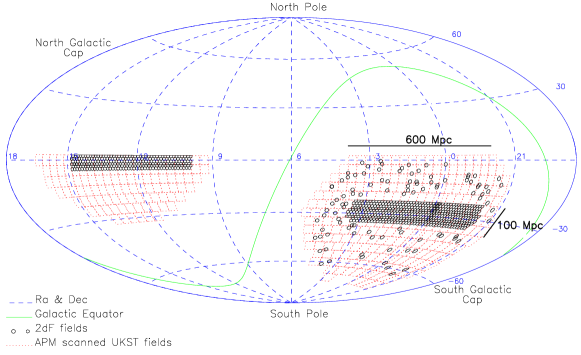
Figure 1: The 2dFGRS fields (small circles) superimposed on the APM catalogue area (dotted outlines of Sky Survey plates). There are approximately 140,000 galaxies in the $75^{\circ}\times 15^{\circ}$ southern strip centred on the SGP, 70,000 galaxies in the $75^{\circ}\times 7.5^{\circ}$ equatorial strip, and 40,000 galaxies in the 100 randomly-distributed 2dF fields covering the whole area of the APM catalogue in the south.

The survey geometry is shown in Figure 1, and consists of two contiguous declination strips, plus 100 random 2-degree fields. One strip is in the southern Galactic hemisphere and covers approximately 75^∘$\times$15^∘ centred close to the SGP at ($\alpha,\delta$)=($01^{h}$,$-30$); the other strip is in the northern Galactic hemisphere and covers $75^{\circ}\times 7.5^{\circ}$ centred at ($\alpha,\delta$)=($12.5^{h}$,$+00$). The 100 random fields are spread uniformly over the 7000 deg² region of the APM catalogue in the southern Galactic hemisphere. At the median redshift of the survey ($\bar{z}=0.11$), $100{\,h^{-1}\,\rm Mpc}$ subtends about 20 degrees, so the two strips are $375{\,h^{-1}\,\rm Mpc}$ long and have widths of $75{\,h^{-1}\,\rm Mpc}$ (south) and $37.5{\,h^{-1}\,\rm Mpc}$ (north).

The sample is limited to be brighter than an extinction-corrected magnitude of $b_{\rm\scriptscriptstyle J}=19.45$ (using the extinction maps of Schlegel et al. 1998). This limit gives a good match between the density on the sky of galaxies and 2dF fibres. Due to clustering, however, the number in a given field varies considerably. To make efficient use of 2dF, we employ an adaptive tiling algorithm to cover the survey area with the minimum number of 2dF fields. With this algorithm we are able to achieve a 93% sampling rate with on average fewer than 5% wasted fibres per field. Over the whole area of the survey there are in excess of 250,000 galaxies.

II Survey Status

By the end of 2000, observations had been made of 161,307 targets in 600 fields, yielding redshifts and identifications for 141,402 galaxies, 7958 stars and 53 QSOs, at an overall completeness of 93%. Repeat observations have been obtained for 10,294 targets. Figure 2 shows the projection of the galaxies in the northern and southern strips onto $(\alpha,z)$ slices. The main points to note are the level of detail apparent in the map and the slight variations in density with R.A. due to the varying field coverage along the strips.

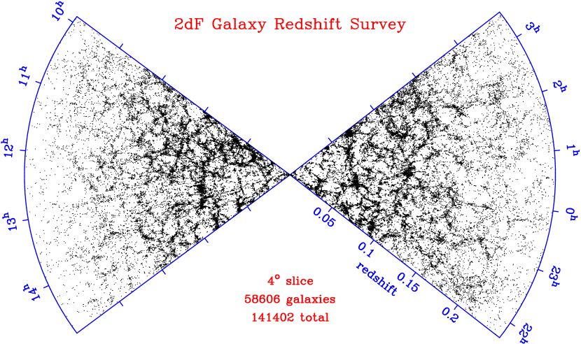
Figure 2: The distribution of galaxies in part of the 2dFGRS, drawn from a total of 141,402 galaxies: slices $4^{\circ}$ thick, centred at declination $-2.5^{\circ}$ in the NGP and $-27.5^{\circ}$ in the SGP. Not all 2dF fields within the slice have been observed at this stage, hence there are weak variations of the density of sampling as a function of right ascension. To minimise such features, the slice thickness increases to $7.5^{\circ}$ between right ascension $13.1^{h}$ and $13.4^{h}$. This image reveals a wealth of detail, including linear supercluster features, often nearly perpendicular to the line of sight. The interesting question to settle statistically is whether such transverse features have been enhanced by infall velocities.

The adaptive tiling algorithm is efficient, and yields uniform sampling in the final survey. However, at this intermediate stage, missing overlaps mean that the sampling fraction has large fluctuations, as illustrated in Figure 3. This variable sampling makes quantification of the large scale structure more difficult, and limits any analysis requiring relatively uniform contiguous areas. However, the effective survey ‘mask’ can be measured precisely enough that it can be allowed for in low-order analyses of the galaxy distribution.

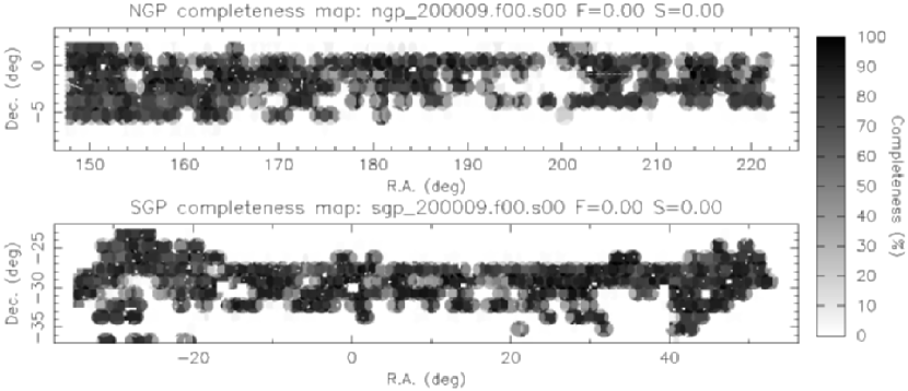
Figure 3: The completeness as a function of position on the sky. The circles are individual 2dF fields (‘tiles’). Unobserved tiles result in low completeness in overlap regions. Rectangular holes are omitted regions around bright stars.

III Redshift-space correlations

The simplest statistic for studying clustering in the galaxy distribution is the the two-point correlation function, $\xi(\sigma,\pi)$. This measures the excess probability over random of finding a pair of galaxies with a separation in the plane of the sky $\sigma$ and a line-of-sight separation $\pi$. Because the radial separation in redshift space includes the peculiar velocity as well as the spatial separation, $\xi(\sigma,\pi)$ will be anisotropic. On small scales the correlation function is extended in the radial direction due to the large peculiar velocities in non-linear structures such as groups and clusters – this is the well-known ‘Finger-of-God’ effect. On large scales it is compressed in the radial direction due to the coherent infall of galaxies onto mass concentrations – the Kaiser effect (Kaiser 1987).

To estimate $\xi(\sigma,\pi)$ we compare the observed count of galaxy pairs with the count estimated from a random distribution following the same selection function both on the sky and in redshift as the observed galaxies. We apply optimal weighting to minimise the uncertainties due to cosmic variance and Poisson noise. This is close to equal-volume weighting out to our adopted redshift limit of $z=0.25$. We have tested our results and found them to be robust against the uncertainties in both the survey mask and the weighting procedure. The redshift-space correlation function for the 2dFGRS computed in this way is shown in Figure 4. The correlation-function results display very clearly the two signatures of redshift-space distortions discussed above. The ‘fingers of God’ from small-scale random velocities are very clear, as indeed has been the case from the first redshift surveys (e.g. Davis & Peebles 1983). However, this is the first time that the large-scale flattening from coherent infall has been seen in detail.

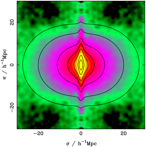
Figure 4: The galaxy correlation function $\xi(\sigma,\pi)$ as a function of transverse ($\sigma$) and radial ($\pi$) pair separation is shown as a greyscale image. It was computed in $0.2{\,h^{-1}\,\rm Mpc}$ boxes and then smoothed with a Gaussian having an rms of $0.5{\,h^{-1}\,\rm Mpc}$. The contours are for a model with $\beta=0.4$ and $\sigma_{p}=400{\,\rm km\,s^{-1}}$, and are plotted at $\xi=10$, 5, 2, 1, 0.5, 0.2 and 0.1.

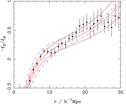
Figure 5: (a) The compression of $\xi(\sigma,\pi)$ as measured by its quadrupole-to-monopole ratio, plotted as $-\xi_{2}/\xi_{0}$. The solid lines correspond to models with $\sigma_{p}=400{\,\rm km\,s^{-1}}$ and (bottom to top) $\beta=0.3$,0.4,0.5, while the dot-dash lines correspond to models with $\beta=0.4$ and (top to bottom) $\sigma_{p}=300,400,500{\,\rm km\,s^{-1}}$. (b) Likelihood contours for $\beta$ and $\sigma_{p}$ from the model fits. The inner contour is the one-parameter 68% confidence ellipse; the outer contours are the two-parameter 68%, 95% and 99% confidence ellipses. The central dot is the maximum likelihood fit, with $\beta=0.43$ and $\sigma_{p}=385{\,\rm km\,s^{-1}}$.

The degree of large-scale flattening is determined by the total mass density parameter, $\mathchar 28682\relax$, and the biasing of the galaxy distribution. On large scales, it should be correct to assume a linear bias model, so that the redshift-space distortion on large scales depends on the combination $\beta\equiv\mathchar 28682\relax^{0.6}/b$. On these scales, linear distortions should also be applicable, so we expect to see the following quadrupole-to-monopole ratio in the correlation function:

$$\frac{\xi_{2}}{\xi_{0}}=\frac{3+n}{n}\frac{4\beta/3+4\beta^{2}/7}{1+2\beta/3+\beta^{2}/5}$$ (1)

where $n$ is the power spectrum index of the fluctuations, $\xi\propto r^{-(3+n)}$. This is modified by the Finger-of-God effect, which is significant even at large scales and dominant at small scales. The effect can be modelled by introducing a parameter $\sigma_{p}$, which represents the rms pairwise velocity dispersion of the galaxies in collapsed structures, $\sigma_{p}$ (see e.g. Ballinger et al. 1996). Full details of the fitting procedure are given in Peacock et al. (2001).

Figure 5a shows the variation in $\xi_{2}/\xi_{0}$ as a function of scale. The ratio is positive on small scales where the Finger-of-God effect dominates, and negative on large scales where the Kaiser effect dominates. The best-fitting model (considering only the quasi-linear regime with $8<r<25{\,h^{-1}\,\rm Mpc}$) has $\beta\simeq 0.4$ and $\sigma_{p}\simeq 400{\,\rm km\,s^{-1}}$; the likelihood contours are shown in Figure 5b. Marginalising over $\sigma_{p}$, the best estimate of $\beta$ and its 68% confidence interval is

$$\beta=0.43\pm 0.07$$ (2)

This is the first precise measurement of $\beta$ from redshift-space distortions; previous studies have shown the effect to exist (e.g. Hamilton, Tegmark & Padmanabhan 2000; Taylor et al. 2000; Outram, Hoyle & Shanks 2000), but achieved little more than 3$\sigma$ detections.

IV Cosmological parameters and the power spectrum

The detailed measurement of the signature of gravitational collapse is the first major achievement of the 2dFGRS; we now consider the quantitative implications of this result. The first point to consider is that there may be significant corrections for luminosity effects. The optimal weighting means that our mean luminosity is high: it is approximately 1.9 times the characteristic luminosity, $L^{*}$, of the overall galaxy population (Folkes et al. 1999). Benoist et al. (1996) have suggested that the strength of galaxy clustering increases with luminosity, with an effective bias that can be fitted by $b/b^{*}=0.7+0.3(L/L^{*})$. This effect has been controversial (see Loveday et al. 1995), but the 2dFGRS dataset favours a very similar luminosity dependence. We therefore expect that $\beta$ for $L^{*}$ galaxies will exceed our directly measured figure. Applying a correction using the given formula for $b(L)$, we deduce $\beta(L=L^{*})=0.54\pm 0.09.$ Finally, the 2dFGRS has a median redshift of 0.11. With weighting, the mean redshift in the present analysis is $\bar{z}=0.17$, and our measurement should be interpreted as $\beta$ at that epoch. The extrapolation to $z=0$ is model-dependent, but probably does not introduce a significant change (Carlberg et al. 2000).

Our measurement of $\mathchar 28682\relax^{0.6}/b$ would thus imply $\mathchar 28682\relax=0.36\pm 0.10$ if $L^{*}$ galaxies are unbiased, but it is difficult to justify such an assumption. In principle, the details of the clustering pattern in the nonlinear regime allow the $\mathchar 28682\relax-b$ degeneracy to be broken (Verde et al. 1998), but for the present it is interesting to use an independent approach. Observations of CMB anisotropies can in principle measure almost all the cosmological parameters, and Jaffe et al. (2000) obtained the following values for the densities in collisionless matter ($c$), baryons ($b$), and vacuum ($v$): $\mathchar 28682\relax_{c}+\mathchar 28682\relax_{b}+\mathchar 28682\relax_{v}=1.11\pm 0.07$, $\mathchar 28682\relax_{c}h^{2}=0.14\pm 0.06$, $\mathchar 28682\relax_{b}h^{2}=0.032\pm 0.005$, together with a power-spectrum index $n=1.01\pm 0.09$. Our result for $\beta$ gives an independent test of this picture, as follows.

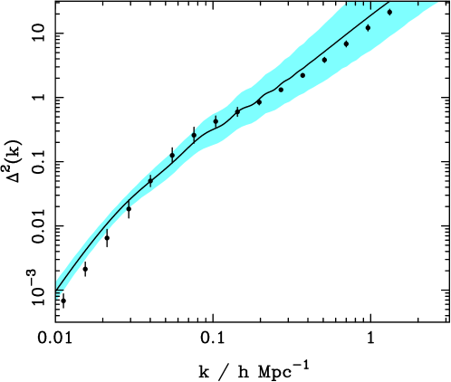
Figure 6: The dimensionless matter power spectrum at zero redshift, $\mathchar 28673\relax^{2}(k)$, as predicted from the allowed range of models that fit the microwave-background anisotropy data, plus the assumption that $H_{0}=70{\,\rm km\,s^{-1}Mpc^{-1}}\pm 10$%. The solid line shows the best-fit model from Jaffe et al. (2000) [power-spectrum index $n=1.01$, and density parameters in baryons, CDM, and vacuum of respectively 0.065, 0.285, 0.760]. The effects of nonlinear evolution have been included, according to a revised version of the procedure of Peacock & Dodds (1996). The shaded band shows the $1\sigma$ variation around this model allowed by the CMB data. The solid points are the real-space power spectrum measured for APM galaxies. The clear conclusion is that APM galaxies are consistent with being essentially unbiased tracers of the mass on large scales.

The only parameter left undetermined by the CMB data is the Hubble constant, $h$. Recent work (Mould et al. 2000; Freedman et al. 2000) indicates that this is now determined to an rms accuracy of 10%, and we adopt a central value of $h=0.70$. This completes the cosmological model, requiring a total matter density parameter $\mathchar 28682\relax\equiv\mathchar 28682\relax_{c}+\mathchar 28682\relax_{b}=0.35\pm 0.14$. It is then possible to use the parameter limits from the CMB to predict a conservative range for the mass power spectrum at $z=0$, which is shown in Figure 6. A remarkable feature of this plot is that the mass power spectrum appears to be in good agreement with the clustering observed in the APM survey (Baugh & Efstathiou 1994). For each model allowed by the CMB, we can predict both $b$ (from the ratio of galaxy and mass spectra) and also $\beta$ (since a given CMB model specifies $\mathchar 28682\relax$). Considering the allowed range of models, we then obtain the prediction $\beta_{\rm\scriptscriptstyle CMB+APM}=0.57\pm 0.17$. A flux-limited survey such as the APM will have a mean luminosity close to $L^{*}$, so the appropriate comparison is with the 2dFGRS corrected figure of $\beta=0.54\pm 0.09$ for $L^{*}$ galaxies. These numbers are in very close agreement. In the future, the value of $\beta$ will become one of the most direct ways of confronting large-scale structure with CMB studies.

V The 2dFGRS power spectrum

Of course, one may question the adoption of the APM power spectrum, which was deduced by deprojection of angular clustering. The 3D data of the 2dFGRS should be capable of improving on this determination, and we have made a first attempt at doing this, shown in Figure 7. This power-spectrum estimate uses the FFT-based approach of Feldman, Kaiser & Peacock (1994), and needs to be interpreted with care. Firstly, it is a raw redshift-space estimate, so that the power beyond $k\simeq 0.2{\,h\,\rm Mpc^{-1}}$ is severely damped by fingers of God. On large scales, the power is enhanced, both by the Kaiser effect and by the luminosity-dependent clustering discussed above. Finally, the FKP estimator yields the true power convolved with the window function. This modifies the power significantly on large scales (roughly a 20% correction). We have made an approximate correction for this in Figure 7 by multiplying by the correction factor appropriate for a $\mathchar 28672\relax=0.25$ CDM spectrum. The precision of the power measurement appears to be encouragingly high, and the systematic corrections from the window are well specified.

Figure 7: The 2dFGRS redshift-space power spectrum, estimated according to the FKP procedure. The solid points with error bars show the power estimate. The window function correlates the results at different $k$ values, and also distorts the large-scale shape of the power spectrum An approximate correction for the latter effect has been applied. The line shows the real-space power spectrum estimated by deprojection from the APM survey.

The next task is to perform a detailed fit of physical power spectra, taking full account of the window effects. The hope is that we will obtain not only a more precise measurement of the overall spectral shape, as parameterized by $\mathchar 28672\relax$, but will be able to move towards more detailed questions such as the existence of baryonic features in the matter spectrum (Meiksin, White & Peacock 1999). We summarize here results from the first attempt at this analysis (Percival et al. 2001).

The likelihood of each model has been estimated using a covariance matrix calculated from Gaussian realisations of linear density fields for a $\Omega_{m}h=0.2$, $\Omega_{b}/\Omega_{m}=0.15$ CDM power spectrum, for which $\chi^{2}_{\rm min}=34.4$, given an expected value of $28$. The best fit power spectrum parameters are only weakly dependent on this choice. The likelihood contours in $\Omega_{b}/\Omega_{m}$ versus $\Omega_{m}h$ for this fit are shown in Figure 8. At each point in this surface we have marginalized by integrating the Likelihood surface over the two free parameters, $h$ and the power spectrum amplitude. The result is not significantly altered if instead, the modal, or Maximum Likelihood points in the plane corresponding to power spectrum amplitude and $h$ were chosen. The likelihood function is also dependent on the covariance matrix (which should be allowed to vary with cosmology), although the consistency of result from covariance matrices calculated for different cosmologies shows that this dependence is negligibly small. Assuming a uniform prior for $h$ over a factor of 2 is arguably over-cautious, and we have therefore added a Gaussian prior $h=0.7\pm 10\%$. This corresponds to multiplying by the likelihood from external constraints such as the HST key project (Freedman et al. 2000); this has only a minor effect on the results.

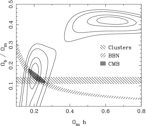
Figure 8: Likelihood contours for the best-fit linear power spectrum over the region $0.02<k<0.15$. The normalization is a free parameter to account for the unknown large scale biasing. Contours are plotted at the usual positions for one-parameter confidence of 68%, and two-parameter confidence of 68%, 95% and 99% (i.e. $-2\ln({\cal L}/{\cal L_{\rm max}})=1,2.3,6.0,9.2$). We have marginalized over the missing free parameters ($h$ and the power spectrum amplitude) by integrating under the Likelihood surface. A prior on $h$ of $h=0.7\pm 10\%$ was assumed. This result is compared to estimates from x-ray cluster analysis (Evrard 1997), big-bang nucleosynthesis (O’Meara et al. 2001) and recent CMB results (Jaffe et al. 2000). The CMB results assume that $\Omega_{b}h^{2}$ and $\Omega_{\rm cdm}h^{2}$ were independently determined from the data.

Figure 8 shows that there is a degeneracy between $\Omega_{m}h$ and the baryonic fraction $\Omega_{b}/\Omega_{m}$. However, there are two local maxima in the likelihood, one with $\Omega_{m}h\simeq 0.2$ and $\sim 20\%$ baryons, plus a secondary solution $\Omega_{m}h\simeq 0.6$ and $\sim 40\%$ baryons. The high-density model can be rejected through a variety of arguments, and the preferred solution is

$$\Omega_{m}h=0.20\pm 0.03;\quad\quad\Omega_{b}/\Omega_{m}=0.15\pm 0.07.$$ (3)

The 2dFGRS data are compared to the best-fit linear power spectra convolved with the window function in Figure 9. This shows where the two branches of solutions come from: the low-density model fits the overall shape of the spectrum with relatively small ‘wiggles’, while the solution at $\Omega_{m}h\simeq 0.6$ provides a better fit to the bump at $k\simeq 0.065{\,h\,\rm Mpc^{-1}}$, but fits the overall shape less well.

Figure 9: The 2dFGRS data compared with the two preferred models from the Maximum Likelihood fits convolved with the window function (solid lines). Error bars show the diagonal elements of the covariance matrix, for the fitted data that lie between the dotted vertical lines. The unconvolved models are also shown (dashed lines). The $\Omega_{m}h\simeq 0.6$, $\Omega_{b}/\Omega_{m}=0.42$, $h=0.7$ model has the higher bump at $k\simeq 0.05{\,h\,\rm Mpc^{-1}}$. The smoother $\Omega_{m}h\simeq 0.20$, $\Omega_{b}/\Omega_{m}=0.15$, $h=0.7$ model is a better fit to the data because of the overall shape.

Perhaps the main point to emphasize here is that the results are not greatly sensitive to the assumed tilt of the primordial spectrum. We have used the CMB results to motivate the choice of $n=1$, but it is clear that very substantial tilts are required to alter our conclusions significantly: $n\simeq 0.8$ would be required to turn zero baryons into the preferred model.

VI Conclusions

The 2dFGRS is now the largest 3D survey of the local universe, by a factor of over 5 compared to any published survey. When it is complete, we expect to have obtained definitive results on a number of key issues relating to galaxy clustering. For details of the current status of the 2dFGRS, see http://www.mso.anu.edu.au/2dFGRS. In particular, this site gives details of the 2dFGRS public release policy, in which we intend to release approximately the first half of the survey data by mid-2001, with the complete survey database to be made public by mid-2003.

At present, the 2dFGRS data allow the galaxy power spectrum to be measured to high accuracy (10–15% rms) over about a decade in scale at $k<0.15{\,h\,\rm Mpc^{-1}}$. We have carried out a range of tests for systematics in the analysis and a detailed comparison with realistic mock samples. As a result, we are confident that the 2dFGRS result can be interpreted as giving the shape of the linear-theory matter power spectrum on these large scales, and that the statistical errors and covariances between the data points are known.

By fitting our results to the space of CDM models, we have been able to reach a number of interesting conclusions regarding the matter content of the universe:

(1)         The power spectrum is close in shape to that of a $\Omega_{m}h=0.2$ model, to a tolerance of about 20%.

(2)         Nevertheless, there is sufficient structure in the $P(k)$ data that the degeneracy between $\Omega_{b}/\Omega_{m}$ and $\Omega_{m}h$ is weakly broken. The two local likelihood maxima have $(\Omega_{m}h,\Omega_{b}/\Omega_{m})\simeq(0.2,0.15)$ and $(0.6,0.4)$ respectively.

(3)         Of these two solutions, the preferred one is the low-density solution. The evidence for detection of baryon oscillations in the power spectrum is presently modest, with a likelihood ratio of approximately 3 between the favoured model and the best zero-baryon model. Conversely, a large baryon fraction can be very strongly excluded: $\Omega_{b}/\Omega_{m}<0.28$ at 95% confidence, provided $\Omega_{m}h<0.4$.

(4)         These conclusions do not depend strongly on the value of $h$, but they do depend on the tilt of the primordial spectrum, with $n\simeq 0.8$ being required to make a zero-baryon model the best fit.

(5)         The sensitivity to tilt emphasizes that the baryon signal comes in good part from the overall shape of the spectrum. Although the eye is struck by a single sharp ‘spike’ at $k\simeq 0.065{\,h\,\rm Mpc^{-1}}$, the correlated nature of the errors in the $P(k)$ estimate means that such features tend not to be significant in isolation. We note that the convolving effects of the window would require a very substantial spike in the true power in order to match our data exactly. This is not possible within the compass of conventional models, and the conservative conclusion is that the apparent spike is probably enhanced by correlated noise. A proper statistical treatment is essential in such cases.

It is interesting to compare these conclusions with other constraints. According to Jaffe et al. (2000), the current CMB data require $\Omega_{m}h^{2}=0.17\pm 0.06$, $\Omega_{b}h^{2}=0.032\pm 0.005$, together with a power-spectrum index of $n=1.01\pm 0.09$, on the assumption of pure scalar fluctuations. If we take $h=0.7\pm 10\%$, this gives

$$\Omega_{m}h=0.24\pm 0.09;\quad\quad\Omega_{b}/\Omega_{m}=0.19\pm 0.07,$$ (1)

in remarkably good agreement with the estimate from the 2dFGRS

$$\Omega_{m}h=0.20\pm 0.03;\quad\quad\Omega_{b}/\Omega_{m}=0.15\pm 0.07.$$ (2)

Latest estimates of the Deuterium to Hydrogen ratio in QSO spectra combined with big-bang nucleosynthesis theory predict $\Omega_{b}h^{2}=0.0205\pm 0.0018$ (O’Meara et al. 2001), which disagrees with the CMB measurement at about the 2$\sigma$ level. The confidence interval estimated from the 2dFGRS power spectrum overlaps both regions. X-ray cluster analysis predicts a baryon fraction $\Omega_{b}/\Omega_{m}=0.127\pm 0.017$ (Evrard 1997) which is again within $1\sigma$ of our preferred value.

The above limits are all shown on Figure 9, and paint a picture of qualitative consistency: it appears that we live in a universe that has $\Omega_{m}h\simeq 0.2$ with a baryon fraction of approximately $15\%$. It is hard to see how this conclusion can be seriously in error. Although the CDM model is claimed to have problems in matching galaxy-scale observations, it clearly works extremely well on large scales. Any new model that cures the small-scale problems will have to look very much like $\Omega_{m}=0.3$ $\Lambda$CDM on large scales.

References

Ballinger W.E., Peacock J.A., Heavens A.F., 1996, MNRAS, 282, 877

Baugh C.M., Efstathiou G., 1994, MNRAS, 267, 323

Benoist C., Maurogordato S., da Costa L.N., Cappi A., Schaeffer R., 1996, ApJ, 472, 452

Carlberg R.G., Yee H.K.C., Morris S.L., Lin H., Hall P.B., Patton D., Sawicki M., Shepherd C.W., 2000, ApJ, 542, 57

Davis M., Peebles, P.J.E., 1983, ApJ, 267, 465

Folkes S.J. et al., 1999, MNRAS, 308, 459

Feldman H.A., Kaiser N., Peacock J.A., 1994, ApJ, 426, 23

Freedman W.L. et al., 2000, astro-ph/0012376

Hamilton A.J.S., Tegmark M., Padmanabhan N., 2000, MNRAS, 317, L23

Jaffe A. et al., 2000, astro-ph/0007333

Kaiser N., 1987, MNRAS, 227, 1

Lewis I., Taylor K., Cannon R.D., Glazebrook K., Bailey J.A., Farrell T.J., Lankshear A., Shortridge K., Smith G.A., Gray P.M., Barton J.R., McCowage C., Parry I.R., Stevenson J., Waller L.G., Whittard J.D., Wilcox J.K., Willis K.C., 2001, MNRAS, submitted

Loveday J., Maddox S.J., Efstathiou G., Peterson B.A., 1995, ApJ, 442, 457

Maddox S.J., Efstathiou G., Sutherland W.J., Loveday J., 1990a, MNRAS, 242, 43p

Maddox S.J., Sutherland W.J., Efstathiou G., Loveday J., 1990b, MNRAS, 243, 692

Maddox S.J., Efstathiou G., Sutherland W.J., 1990c, MNRAS, 246, 433

Meiksin A.A., White M., Peacock J.A., 1999, MNRAS, 304, 851

Mould J.R. et al., 2000, ApJ, 529, 786

Outram P.J., Hoyle F., Shanks T., 2000, astro-ph/0009387

Peacock J.A., Dodds S.J., 1996, MNRAS, 280, L19

Peacock J.A. et al., 2001, Nature, 410, 169

Percival W.J. et al., 2001, MNRAS, submitted

Schlegel D.J., Finkbeiner D.P., Davis M., 1998, ApJ, 500, 525

Taylor A.N., Ballinger W.E., Heavens A.F., Tadros H., 2000, astro-ph/0007048

Verde L., Heavens A.F., Matarrese S., Moscardini L., 1998, MNRAS, 300 747