Synthetic Doppler maps of gaseous flows in IP Peg
Abstract
We present synthetic Doppler maps of gaseous flows in binary IP Peg based on the results of 3D gasdynamical simulations. Using of gasdynamical calculations alongside with the Doppler tomography technique permits us to identify the main features of the flow on the Doppler maps without solution of an ill-posed inverse problem. Comparison of synthetic tomograms with observations shows that in quiescence there are two zones of high emission: a shock wave on the edge of the stream from caused by the interaction of the gas of circumbinary envelope and the stream, and the dense region in a apoastron of quasi-elliptical accretion disk. A single arm of the spiral shock and the stream itself give a minor input to the total brightness. During outburst the accretion disk dominates, and the most emitive regions are the two arms of the spiral shock.
1 Introduction
Traditional observations of binary systems are carried out using photometric and spectroscopic methodics. The former gives the time dependence of brightness in a specific band and the latter can give the time dependence of wavelength of some Doppler-shifted line . Given ephemeris is known, the dependencies and can be converted by virtue of Doppler formula to the light curve and the phase dependency of radial velocity .
During the last ten years the observations of binary systems in the form of trailed spectrograms for some emission line (or in other terms ) become widely used. A method of Doppler tomography (Marsh & Horne 1988) is suited to analyze the trailed spectrograms. Using this method one can obtain a map of luminosity in the 2D velocity space from the orbital variability of emission lines intensity. The Doppler tomogram is constructed as a conversion of time resolved (i.e. phase-folded) line profiles into the map on (, ) plane. To convert the distribution into the Doppler map we should use the expression for radial velocity as a projection of velocity vector on the line of sight, i.e. (here we assume that , the minus sign before is taken for consistency with the coordinate system), and solve an inverse problem that is described by integral equation (see Appendix A of Marsh & Horne 1988):
| (1) |
where is a normalized local line profile (e.g., the Dirac -function), and the limits of integration are from to . This inverse problem is ill-posed and the special regularization is necessary for its solving (e.g. Maximum Entropy Method, Narayan & Nityananda 1986, Marsh & Horne 1988; Fourier Filtered Back Projection, Robinson, Marsh & Smak 1993; Fast Maximum Entropy Method, Spruit 1998; etc., see also Frieden 1979).
As a result we obtain a map of distribution of specific line intensity in velocity space. This map is easier to interpret than original line profiles, moreover, the tomogram can show (or at least gives a hint to) some features of flow structure. In particular, the double-peaked line profiles corresponding to circular motion of the gas (e.g. in accretion disk) become a diffuse ring-shaped region in this map. Resuming, we can say that components of binary system can be resolved in velocity space while they can not be spatially resolved through direct observations, so the Doppler tomography technique is a rather power tool for studying of binary systems.
Unfortunately, the reconstruction of the spatial distribution of intensity on the basis of a Doppler map is an ambiguous problem since the points located far from each other may have equal radial velocities and deposit to the same pixel on the Doppler map. So the transformation is impossible without some a priori assumptions on the velocity field.
The situation changes drastically when one uses gasdynamical calculations alongside with Doppler tomography technique. In this case we don’t need to cope with the inverse problem since the task is solved directly: and . Difficulties can arise when converting the spatial distributions of density and temperature , into the distribution of luminosity of specific emission line . For optically thick lines the formation of line profile should be described by radiation transfer equations (see, e.g., Horne & Marsh 1986), therefore to produce synthetic Doppler maps we assume that the matter is optically thin and the intensity of considered recombination line is as (Ferland 1980; Richards & Ratliff 1998).
2 Binary system parameters
The variable star IP Peg was discovered by Lipovetskij and Stepanyan (1981). It was found to be an eclipsing dwarf nova (orbital period ) with a deep eclipse and a hump on the light curve by Goransky et al. (1985).
A binary system can be completely described by the following set of parameters: orbital period , masses of the components and , separation , and inclination angle . Among all parameters only is determined immediately from observations while parameters , , , (or in another statement , , , , where – total mass, – mass ratio) should be calculated from observational data. These parameters are connected by third Kepler’s law (here – angular velocity of the orbital motion; – gravitational constant), so we need only three additional relations.
Several ways of determination of relationships between the parameters of the binary on the basis of observational data are known to exist:
(i) using semi-amplitudes of radial velocity
for mass-losing star and accretor, correspondingly, we can calculate , and set a relation between and ( is considered to be already known);
(ii) using the width of the white dwarf eclipse (for eclipsing binaries only) we can set a relation between and .
Knowing observable entities , , and permits us to determine all parameters of the binary system. Note, that alternate methods of setting of relations between system’s parameters also exist. For example, knowing of rotational broadening of absorbtion lines , (where – effective radius of the Roche lobe) permits set an additional relation between , and . Usage of extra relations can be exploited for checking of input parameters.111Determination of system’s parameters from width of ‘hot spot’ eclipse (see, e.g., Wood & Crawford 1986; Smak 1996) is not considered here since we suggest an essentially different model of the flow structure in semidetached binaries. We also don’t rely on the mass-radius relation since it is determined primarily for single stars.
Semi-amplitudes of radial velocity for white dwarf were determined in Wood & Crawford (1986); Marsh (1988); Marsh & Horne (1990): Marsh (1988) obtained the value of km s-1 (but using Shafter’s method (1983) he obtained a lower value of km s-1), Wood & Crawford (1986) obtained the value of km s-1. Semi-amplitudes of radial velocity for mass-losing star were determined in Martin et al. (1987, 1989); Marsh (1988); Beekman et al. (2000): Marsh (1988) obtained the value of km s-1, Martin et al. (1987, 1989) – the value of km s-1, and Beekman et al. (2000) – the value of km s-1. We adopt the values of semi-amplitudes of radial velocity according to Wood & Crawford (1986) and Marsh & Horne (1990): km s-1, km s-1.

After the values of and are adopted we can exploit the relation between system’s parameters resulting from the value of width of the white dwarf eclipse. This value is known with sufficient accuracy: Wood & Crawford (1986) obtained , and Marsh (1988) obtained . The width of the white dwarf eclipse gives the relation between the orbit inclination and the mass ratio as (see, e.g., Horne, Lanning & Gomer 1982; Dhillon, Marsh & Jones 1991):
| (2) |
Here and are the Roche lobe sizes in and directions ( axis is perpendicular to the orbital plane and axis is directed along the orbital motion of mass-losing star). Usually and functions are taken approximately (Pacyński 1971) as:
| (3) |
Resulting dependency between and for the value is shown in Fig. 1 (dashed line). However, usage of the approximate formula (3) may in this case lead to the loss of accuracy, so we have calculated dependencies and exactly for and approximated it (error ) as
Obtained relationship is shown in Fig. 1 as well (solid line). Besides, we put values and adopted by Wood & Crawford (1986); Marsh (1988); and Beekman et al. (2000).
Using the values for , mentioned above, as well as the more precise dependency we take the parameters for IP Peg as follows: , , . The distance between the inner Lagrangian point and accretor is , the distance between system’s center of mass and accretor is .
These parameters give the rotational broadening of the absorbtion lines of mass-losing star as km s-1. Observational measurements of give km s-1 (Harlaftis 1999) and km s-1 (Catalán, Smith & Jones 2001). Good agreement between calculated and observational parameters in this additional relation bears witness on the correctness of system’s parameters in use.
We would like to stress that there were some factors not included in our model. Martin et al. (1987) and Beekman et al. (2000) point out a possible ellipticity of binary components’ orbits (eccentrisity ). Some authors (Wood et al. 1989; Wolf et al. 1993) argue that some observational peculiarities of IP Peg can be explained by the presence of the third body in the system. In our work we assume that the system contains two stellar components only, its orbits being circular.
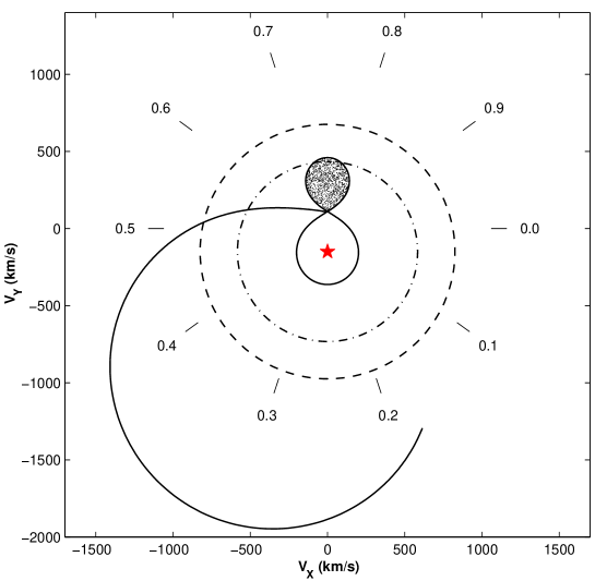
Lower panel: The adopted coordinate system in the velocity space. All designations are the same as in the upper panel.
3 Model
3.1 Gasdynamical model
The full description of the 3D gasdynamical model can be found in Bisikalo et al. (2000). Here we pay attention only to the main features of the model. To describe the gas flow in this binary system we used the 3D system of Euler equations for Cartesian coordinate system. To close the system of equations, we used the equation of state of ideal gas with adiabatic index . To mimic the system with radiative losses, the value of adiabatic index has been accepted close to unit: , that corresponds to the case close to the isothermal one (Sawada, Matsuda & Hachisu 1986, Molteni, Belvedere & Lanzafame 1991; Bisikalo et al. 1995).
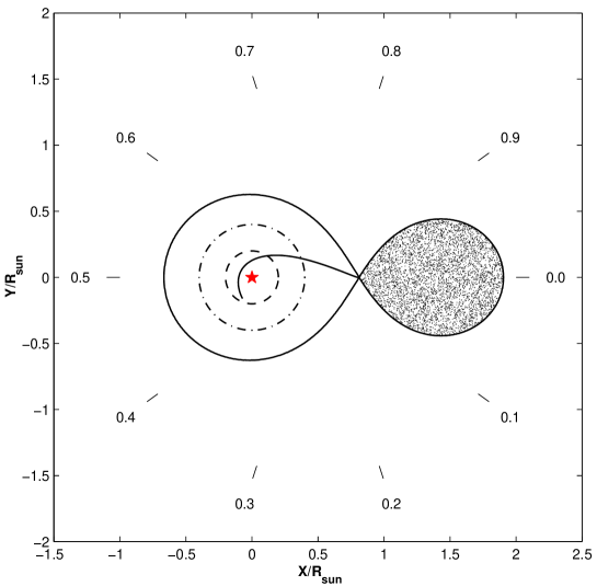
The calculations were carried out in the non-inertial Cartesian coordinate system rotating with the binary system. The results of the calculations and the Doppler tomograms will be presented in coordinate system defined as follows: the origin of coordinates is located in the center of the accretor, -axis is directed along the line connecting the centers of stars, from accretor to the mass-losing component, -axis is directed in the direction of orbital movement of the donor-star, -axis is directed along the axis of rotation, so we obtain a right-hand coordinate system. Figure 2 (top panel) shows the coordinate system. In this figure we also put digits showing the phase angles of the observer in binary system, a Roche lobe with shadowed donor-star and the ballistic trajectory of a particle moving from point to the accretor. The adopted coordinate system for Doppler maps is shown in the lower panel of Fig. 2. The transformation of the donor-star from spatial to velocity coordinate system is very simple as it is fixed in the corotating frame. Every point fixed in the binary frame has a velocity in the corotation frame. This expression is linear in the perpendicular distance from the rotation axis, therefore the shape of the donor-star projected on the orbital plane is preserved. Since the velocity of each point of the donor-star is perpendicular to the radius vector, all points of the donor-star are rotated by 90∘ counter-clockwise between the spatial and velocity coordinate diagrams (shadowed regions on the top and lower panels of Fig. 2, see also Marsh & Horne 1988). On the velocity plane the accretor has coordinates (0,). Figure 2 also depicts two concentric circles corresponding to different radii of the disk and their representations on the velocity plane (for Keplerian rotation law). Inner circle has a larger velocity and forms the outer circle on the Doppler tomogram.
To obtain numerical solution of the system of equations we used the Roe–Osher TVD scheme of a high approximation order (Roe 1986; Chakravarthy & Osher 1985) with Einfeldt modification (Einfeldt 1988). The computational domain was taken as a parallepipedon (due to the symmetry of the problem calculations were conducted only in the top half-space). A sphere with a radius of representing the accretor was cut out of the calculation domain. The boundary conditions were taken as ‘free outflow’ on the accretor star and on the outer edges of computational domain. In the gridpoint corresponding to we injected the matter with parameters , , , where is a gas speed of sound in point. Due to the scaling of the system of equations with respect to (with simultaneous scaling of pressure ) we can accept an arbitrary value of so we take it as .222When considering a system with known mass-loss rate, to determine the real values it is necessary to change the calculated values of density in accordance with the scale, defined by the ratio of the real value of the mass loss rate to the model one. The sound speed in was adopted as 5.5 km s-1 which corresponds to K. For the initial conditions we used rarefied gas with the following parameters , , .
3.2 Technique for construction of synthetic Doppler tomograms
Preceding the consideration of the synthetic Doppler tomograms for binary system IP Peg it is necessary to stress the complexity of the analysis of these tomograms for eclipsing systems (see, e.g., Kaitchuck et al. 1994). The concept of Doppler tomography implies that any geometrical point deposits in some place on the velocity plane, this point being visible for any orbital phase. Indeed, from (1) we have
i.e. the constructions of synthetic Doppler tomograms is possible only for those sets of trailed spectrograms which are transformed symmetrically when one sees the binary system from the “dark side” or, in other words, when there are no eclipses and occultations of emission regions. Clearly, eclipsing systems violates that assumption. Usually, when dealing with observations, the eclipsed parts of trailed spectrograms are naturally excluded from input data for construction of Doppler tomograms. As a result, we obtain the Doppler map corresponding to the “transparent” case. The conversion of the results of gasdynamical simulation into Doppler maps suggests using of full set of data that also corresponds to the “transparent” case.
The Doppler maps show the distribution of luminosity in the velocity space. Each point of the flow has a three-dimensional vector of velocity in observer’s (inertial) frame. In the case when observer is located in the orbital plane of the binary the Doppler map’s coordinate will coincide with and . To define these coordinates for the case of inclined system we have to find a projection of vector on the plane constituted by vectors and , where is a direction from the observer to binary.
The line emissivity in the velocity space can be written as:
| (4) |
where , – inclination angle.
As was mentioned above we adopt intensity as for the construction of synthetic Doppler tomograms.
4 Results for quiescence of IP Peg
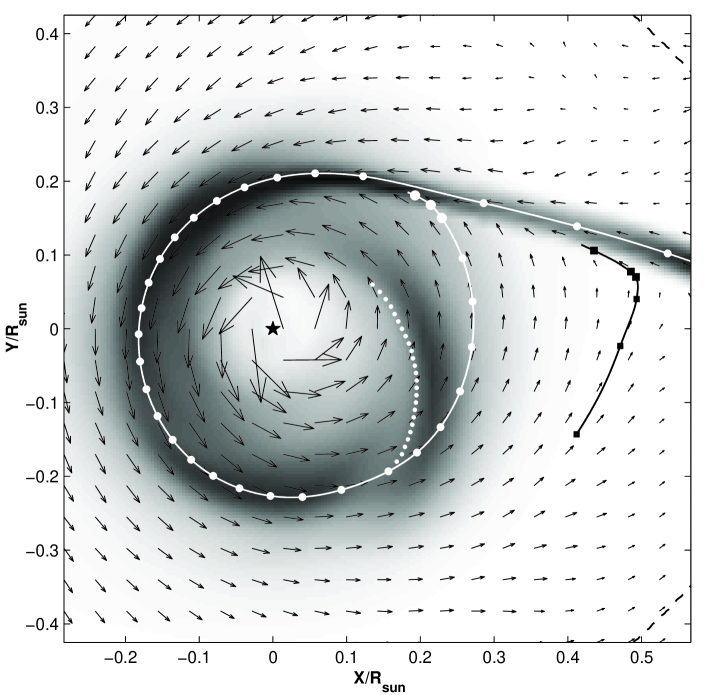
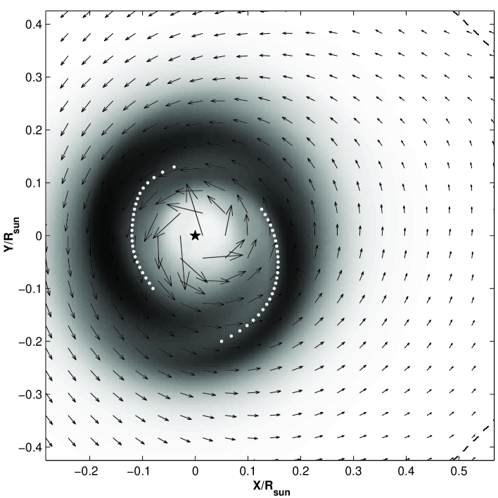
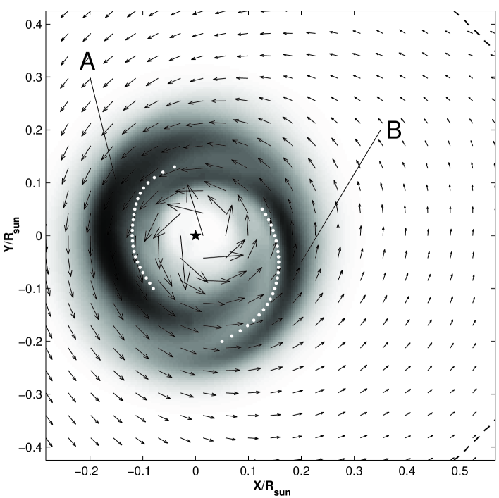
Based on the model described in the Section 4.1 we have conducted the 3D gasdynamical simulation of IP Peg in quiescence up to reaching of a steady-state solution. The morphology of gaseous flows in considered binary system can be evaluated from Figs 3a. In Fig. 3a the distribution of density over the equatorial plane and velocity vectors are presented. In this Figure we also put a gasdynamical trajectory of a particle moving from to accretor (a white line with circles) and a gasdynamical trajectory passing through the shock wave along the stream edge (a black line with squares, see also Fig. 4). Analysis of the presented results as well as our previous studies (Bisikalo et al. 1997, 1998b) shows the significant influence of the rarefied gas of circumbinary envelope on the flow patterns in semidetached binaries. The gas of circumbinary envelope interacts with the stream of matter and deflects it. This leads, in particular, to the shock-free (tangential) interaction between the stream and the outer edge of forming accretion disc, and, as the consequence, to the absence of ‘hot spot’ in the disc.
At the same time it is seen, that the interaction of the gas of circumbinary envelope with the stream results in the formation of an extended shock wave located along the stream edge (‘hot line’). The ‘hot line’ model was confirmed by confronting with observations (see Bisikalo et al. 1998a; Khruzina et al. 2001). From Fig. 3a it is also seen the formation of tidally induced spiral shock (white dotted line in Fig. 3a). Appearance of the tidally induced two-armed spiral shock was numerically discovered in Sawada, Matsuda & Hachisu (1986a, 1986b); Sawada et al. (1987); Spruit et al. (1987); Matsuda et al. (1990). Here we see only the one-armed spiral shock. In the place where the second arm should be the stream from dominates and presumably prevents the formation of second arm of tidally induced spiral shock.
An analysis of the flow structure out of equatorial plane shows that a part of the circumbinary envelope interacts with the (denser) gas stream and overflows it. This naturally leads to the formation of ‘halo’. Following to (Bisikalo et al. 2000), one can define ‘halo’ as that matter which: i) encircles the accretor being gravitationally captured; ii) does not belong to the accretion disc; iii) interacts with the stream (collides with it and/or overflows it); iv) after the interaction either becomes a part of the accretion disc or leaves the system.
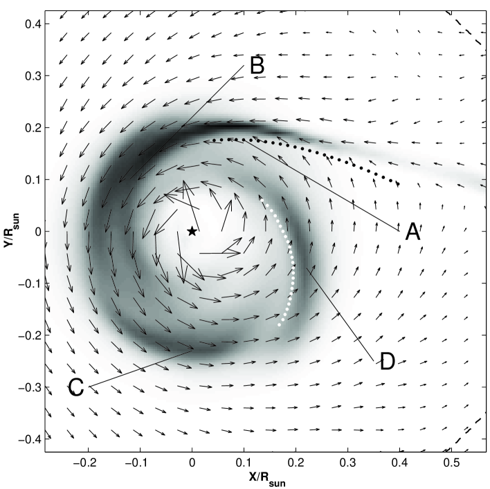
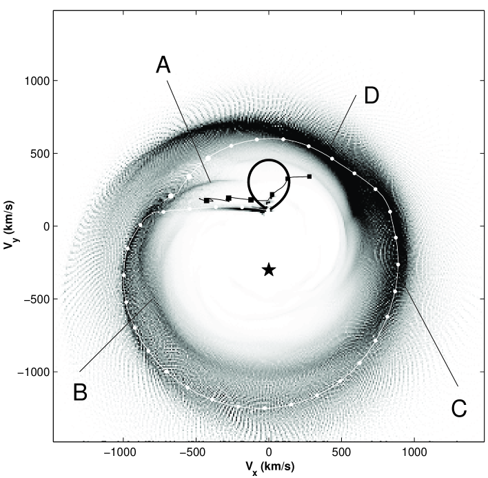
Figure 3b depicts the distribution of over the equatorial plane. Similar to Fig. 3a spiral shock is shown by white dotted line. Besides, shock wave along the edge of the stream is shown by black dotted line. The distribution shown in Fig. 3b represents the intensity of recombination line, so the analysis of this distribution can determine the most luminous region of the flow. It is seen, that the main emission comes from four region designated by markers A, B, C, D.
-
•
Marker A designates the shock wave along the edge of the stream (‘hot line’) resulting from the gasdynamical interaction of the gas of circumbinary envelope with the stream.
-
•
Marker B designates the stream from or, more exactly, the most luminous part of the stream where the density is still large enough and the temperature already increases due to dissipation.
-
•
Marker C designates a region near the apoastron of the accretion disk. The analysis of the presented results shows that the disk has a quasi-elliptical form, therefore approaching the apoastron the matter is retarded and the dense region is formed.
-
•
Marker D designates a dense post-shock region attached to the spiral shock.
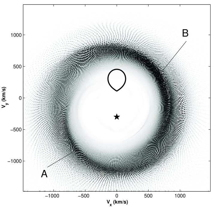
The synthetic Doppler map based on the results of 3D gasdynamical simulations is presented in Fig. 4. Earlier we have analyzed the features of flow in the equatorial plane (see Figs 3a, 3b), but for the sake of comparison with observations synthetic Doppler maps will be presented for integrated over -coordinate intensity in accordance to the equation (4). Two gasdynamical trajectories (the same as in Fig. 3a but in velocity coordinates) are shown in Fig. 4.
Shock wave resulting from the gasdynamical interaction of the gas of circumbinary envelope with the stream is located along the edge of the stream. Three last points (marked by larger symbols) of curves with circles and squares in Fig. 3a are the examples of two flowlines passing through the shock. Location of these parts of trajectories on the Doppler map corresponds to region A left to the donor-star. This region of Doppler map contains also a spiral arm beginning approximately from the center of mass-losing star and located above the vicinity of . Our analysis shows that the appearance of this region results from the overflowing the stream by the gas of circumbinary envelope but not from the shock wave. It is seen from Fig. 4 that the stream from (the beginning of white line whit circles) transforms into spiral arm B in III quadrant333The quadrants of coordinates plane are counted as follows: I quadrant is upper right (corresponding to , ), other quadrants are counted counter-clockwise. of the Doppler map. The region of increased density near apoastron of the disk – region C is seen in Fig. 4 as more luminous zone on the border of I and IV quadrants. Tidally induced spiral shock (or, more exactly, the dense post-shock zone, dotted line in Figs 3a, 3b) forms a bright arm in I and II quadrants of Doppler map.
Resuming these results for Doppler map of IP Peg in quiescence we can conclude that there are four elements of the flow structure which deposit in the total luminosity: ‘hot line’, the most luminous part of the stream where, the dense region near the apoastron of the disk, and the dense post-shock region attached to the spiral shock. The income of each element obviously can vary depending on peculiarities of considered binary system. It is also obvious that based on the model computations we can’t estimate what elements will dominate. Nevertheless, comparison of synthetic Doppler maps and observed ones permits both to catch the dominating element and to correct/refine the computational model.
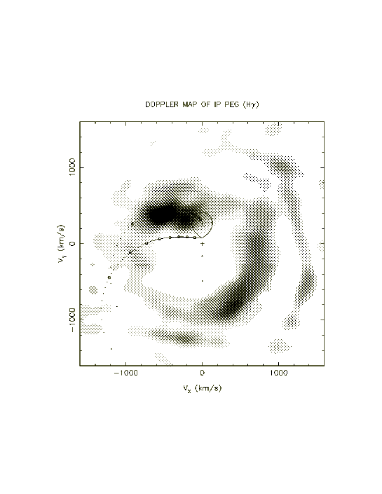
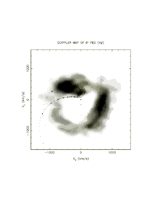
Observational Doppler tomograms for IP Peg in quiescence were built in Marsh & Horne (1990); Harlaftis et al. (1994); Wolf et al. (1998); Bobinger et al. (1999); Bobinger (2000). Figure 5 represents a typical Doppler map for Hγ and Hβ from Wolf et al. (1998). The characteristic features of these tomograms are the bright spot in the region A as well as the zone of moderate brightness in the region C. The comparison of the observational tomogram from Fig. 5 and synthetic one from Fig. 4 reveals that it is the ‘hot line’ and the dense zone near the disk’s apoastron which mainly deposit into the total luminosity. Signatures of the spiral shock are not seen and this implies either its absence or weakness. Note also that the observational tomogram shows rather small input from the stream from into the total luminosity.
5 Results for outburst of IP Peg
Observations show (see, e.g., recent reviews by Marsh 2000 and Steeghs 2000) that during outburst the accretion disk dominates hence the stream from plays less important role. Our today’s knowledge of the nature of the outburst as well as its parameters has an approximate and qualitative character so it is hard to simulate the outburst correctly. To mimic the flow structure during outburst on the qualitative level we calculated the structure of gaseous flows up to reaching a quasi-steady-state solution and put the rate of mass transfer equal to zero (i.e. terminated the mass transfer) as it was suggested in Bisikalo et al. (2001a, 2001b). We understand that this model doesn’t reflect all peculiarities of outburst and expanding accretion disk but we hope that it truly correlates the influence the disk and the stream on the qualitative level. Our simulations of residual accretion disk show that at time after mass transfer termination the flow structure is changed significantly. The stream from vanishes and doesn’t dominate anymore, and the shape of accretion disk changes from quasi-elliptical to circular. The second arm of tidally induced spiral shock is formed while earlier (before the termination of mass transfer) it was suppressed by the stream from . It is seen that obtained flow structure has all basic features observed in outburst of IP Peg. This gives a hope that we can refine/reveal the new features of IP Peg in outburst by virtue of analysis of synthetic Doppler tomograms constructed for this gasdynamical solution.
Figure 6a depicts the distribution of density and velocity vectors and Fig. 6b depicts the distribution of over the equatorial plane. It is seen, that the main emission comes from two arms of the spiral shock designated by markers A and B. The synthetic Doppler map based on the results of 3D gasdynamical simulations for IP Peg in outburst is presented in Fig. 7. Our analysis shows that bright arms in I and III quadrants are due to emission of dense post-shock zones attached to the arms of spiral shock.
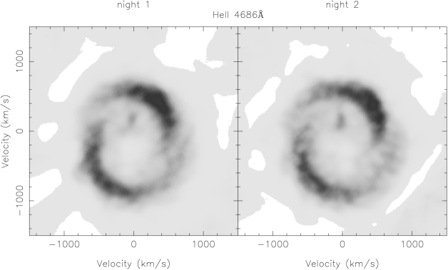
Observational Doppler tomograms for IP Peg during the outburst were built in Marsh & Horne (1990); Steeghs et al. (1996); Steeghs, Harlaftis & Horne (1997); Harlaftis et al. (1999); Morales-Rueda, Marsh & Billington (2000). A typical example of such tomogram (Morales-Rueda, Marsh & Billington 2000) is given in Fig. 8. The characteristic features of these tomograms are two bright arms in I and III quadrants. The comparison of the observational tomogram from Fig. 8 and synthetic one from Fig. 7 reveals that these arms results from dense post-shock zones attached to the arms of spiral shock (zones A and B).
6 Conclusions
Using of the gasdynamical calculations alongside with Doppler tomography technique permits us to identify main features of the flow on the Doppler maps without solution of the ill-posed inverse problem. The comparison of synthetic Doppler maps and observed ones permits to correct/refine the computational model and to interpret the observational data. In this work we have presented the synthetic Doppler maps of gaseous flows in binary IP Peg based on the results of 3D gasdynamical simulations. The zones of flow structure responsible for the most emitive regions of Doppler map were identified and it was found that they are different for quiescence and outburst. Our analysis for quiescence has shown that it is the shock wave along the stream edge – ‘hot line’ and the dense zone near the disk’s apoastron which mainly deposit into the total luminosity. The input from the stream from and the spiral shock into the total luminosity is small. During the outburst the role of the stream is unimportant and the accretion disk with two-armed spiral shock dominates. The comparison of the observational tomogram and synthetic one reveals that the bright arms in the Doppler map result from dense post-shock zones attached to the arms of the spiral shock.
Acknowledgments
The work was partially supported by Russian Foundation for Basic Research (projects NN 99-02-17619, 99-02-17589, 00-01-00392, 00-02-16471, 00-02-17253), by grants of President of Russia (99-15-96022, 00-15-96722, 00-15-96553), and by INTAS (grant 01-491). Authors wish to thank V.V.Neustroev for useful discussions on observational Doppler tomograms.
References
- [1]
- [2] Beekman G., Somers M., Naylor T., Hellier C. 2000, A TiO Study of the Dwarf Nova IP Peg, Monthly Notices Roy. Astron. Soc., 318, 9
- [3] Bisikalo D.V., Boyarchuk A.A., Kuznetsov O.A., Popov Yu.P., Chechetkin V.M. 1995, Structure of the Accretion Disk in Symbiotic Stars. The Isothermal Case, Astron. Zh., 72, 367 (Astron. Reports, 39, 325)
- [4] Bisikalo D.V., Boyarchuk A.A., Kuznetsov O.A., Chechetkin V.M. 1997, Three-dimensional Modeling of the Matter Flow Structure in Semidetached Binary Systems, Astron. Zh., 74, 880 (Astron. Reports, 41, 786, preprint astro-ph/9802004)
- [5] Bisikalo D.V., Boyarchuk A.A., Kuznetsov O.A., Khruzina T.S., Cherepashchuk A.M., Chechetkin V.M. 1998a, Evidence for the Absence of a Stream-Disk Shock Interaction in Semi-Detached Binary Systems: Comparison of Mathematical Modeling Results and Observations, Astron. Zh., 75, 40 (Astron. Reports, 42, 33, preprint astro-ph/9802134)
- [6] Bisikalo D.V., Boyarchuk A.A., Chechetkin V.M., Kuznetsov O.A., Molteni D. 1998b, 3D Numerical Simulation of Gaseous Flows Structure in Semidetached Binaries, Monthly Notices Roy. Astron. Soc., 300, 39
- [7] Bisikalo D.V., Boyarchuk A.A., Kuznetsov O.A., Chechetkin V.M. 2000, The Impact of Viscosity on the Flow Structure Morphology in Semidetached Binary Systems. Results of 3D Numerical Modeling, Astron. Zh., 77, 31 (Astron. Reports, 44, 26, preprint astro-ph/9907087)
- [8] Bisikalo D.V., Boyarchuk A.A., Kilpio A.A., Kuznetsov O.A., Chechetkin V.M. 2001a, Structure of Gaseous Flows in Semidetached Binaries after Mass Transfer Termination, Astron. Zh., in press (preprint astro-ph/0102241)
- [9] Bisikalo D.V., Boyarchuk A.A., Kilpio A.A., Kuznetsov O.A. 2001b, On Possible Observational Evidences of Spiral Shocks in Accretion Disks of CVs, Astron. Zh., in press (preprint astro-ph/0105403)
- [10] Bobinger A., Barwig H., Fiedler H., Mantel K.-H., Ŝimić D., Wolf S. 1999, Double Dataset Eclipse Mapping of IP Peg, Astron. Astrophys., 348, 145
- [11] Bobinger A. 2000, General Eclipse Mapping and the Advantage of Black Sheep, Astron. Astrophys., 357, 1170
- [12] Catalán M.S., Smith R.C., Jones D.H.P. 2001, Monthly Notices Roy. Astron. Soc. (in press, see Beekman et al. 2000)
- [13] Chakravarthy S.R., Osher S. 1985, A New Class of High Accuracy TVD Schemes for Hyperbolic Conservation Laws, AIAA Pap., N 85-0363
- [14] Einfeldt B. 1988, On Godunov-Type Methods for Gas Dynamics, SIAM J. Numer. Anal., 25, 294
- [15] Dhillon V.S., Marsh T., Jones D.H.P. 1991, A Spectrophotometric Study of the Eclipsing Nova-like Variable V1315 Aquilae, Monthly Notices Roy. Astron. Soc., 252, 342
- [16] Ferland C.J. 1980, Hydrogenic Emission and Recombination Coefficients for a Wide Range of Temperature and Wavelength, Publ. Astron. Soc. Pacific, 92, 596
- [17] Frieden B.R. 1975, Image Enhancement and Restoration, in “Picture Processing and Digital Filtering”, ed. T.S.Huang, New York: Springer-Verlag, p. 177
- [18] Goranskij V.P., Shugarov S.Yu., Orlowsky E.I., Rahimov V.Yu. 1985, The Dwarf Nova SVS 2549, a Shortperiodic Eclipsing System, Int. Bull. Variable Stars, No.2653
- [19] Harlaftis E.T., Marsh T.R, Dhillon V.S., Charles P.A. 1994, A 60-NIGHT Campaign on Dwarf Novae – II. Evidence for Balmer Emission from the Secondary Star in IP Pegasi Close to Outburst, Monthly Notices Roy. Astron. Soc., 267, 473
- [20] Harlaftis E.T. 1999, Discovery of Metal Line Emission from the Red Star in IP Peg during Outburst Maximum, Astron. Astrophys., 346, L73
- [21] Harlaftis E.T., Steeghs D., Horne K., Martín E., Magazzú A. 1999, Spiral Shocks in the Accretion Disc of IP Peg during Outburst Maximum, Monthly Notices Roy. Astron. Soc., 306, 348
- [22] Horne K., Lanning H.H., Gomer R.H. 1982, A First Look at the Eclipsing Variable Lanning 10, Astrophys. J., 252, 681
- [23] Horne K., Marsh T.R. 1986, Emission Line Formation in Accretion Discs, Monthly Notices Roy. Astron. Soc., 218, 761
- [24] Kaitchuck R.H., Schlegel E.M., Honeycutt R.K., Horne K., Marsh T.R., White J.C.,II, Mansperger C.S. 1994, An Atlas of Doppler Emission-line Tomography of Cataclysmic Variable Stars, Astrophys. J. Suppl., 93, 519
- [25] Khruzina T.S., Cherepashchuk A.M., Bisikalo D.V., Boyarchuk A.A., Kuznetsov O.A. 2001, The Interpretation of Light Curves of IP Peg in the Model of Shock-free Interaction between the Gas Stream and the Disk, Astron. Zh., in press
- [26] Lipovetskij V.A., Stepanyan G.A. 1981, New Variable Stellar Objects with UV-Continuum, Astrofizika, 17, 573
- [27] Marsh T.R., Horne K. 1988, Images of Accretion Discs. II – Doppler Tomography, Monthly Notices Roy. Astron. Soc., 235, 269
- [28] Marsh T.R. 1988, A Spectroscopic Study of the Deeply Eclipsed Dwarf Nova IP Peg, Monthly Notices Roy. Astron. Soc., 231, 1117
- [29] Marsh T.R., Horne K. 1990, Emission-Line Mapping of the Dwarf Nova IP Pegasi in Outburst and Quiescence, Astrophys. J., 349, 593
- [30] Marsh T.R. 2000, Doppler Tomography, in Proceedings of Astro-Tomography Workshop, Brussels, eds H.Boffin, D.Steeghs, J.Cuypers (in press, preprint astro-ph/0011020).
- [31] Martin J.C., Jones D.H.P., Smith R.C., 1987, Spectroscopy and Photometry of IP Peg in the Near-Infrared, Monthly Notices Roy. Astron. Soc., 224, 1031
- [32] Martin J.C., Friend M.T., Smith R.C., Jones D.H.P. 1989, Spectroscopy of the Red Star in IP Peg, Monthly Notices Roy. Astron. Soc., 240, 519
- [33] Matsuda T., Sekino N., Shima E., Sawada K., Spruit H. 1990, Mass Transfer by Tidally Induced Spiral Shocks in an Accretion Disk, Astron. Astrophys., 235, 211
- [34] Molteni D., Belvedere G., Lanzafame G. 1991, Three-dimensional Simulation of Polytropic Accretion Discs, Monthly Notices Roy. Astron. Soc., 249, 748
- [35] Morales-Rueda L., Marsh T.R., Billington I. 2000, Spiral Structure in IP Pegasi: how persistent is it? Monthly Notices Roy. Astron. Soc., 313, 454
- [36] Narayan R., Nityananda R. 1986, Maximum Entropy Image Restoration in Astronomy, Ann. Rev. Astron. Astrophys., 24, 127
- [37] Paczyński B. 1971, Evolutionary Processes in Close Binary Systems, Ann. Rev. Astron. Astrophys., 9, 183
- [38] Richards M.T., Ratliff M.A. 1998, Hydrodynamic Simulations of H Emission in Algol-type Binaries, Astrophys. J., 493, 326
- [39] Robinson E.L., Marsh T.R., Smak J. 1993, The Emission Lines from Accretion Disks in Cataclysmic Variable Stars, in “Accretion Disks in Compact Stellar Systems”, ed. J.C.Wheeler, Singapore: World Sci. Publ., p. 75
- [40] Roe P.L. 1986, Characteristic-Based Schemes For the Euler Equations, Ann. Rev. Fluid Mech., 18, 337
- [41] Sawada K., Matsuda T., Hachisu I. 1986a, Spiral Shocks on a Roche Lobe Overflow in Semidetached Binary System, Monthly Notices Roy. Astron. Soc., 219, 75
- [42] Sawada K., Matsuda T., Hachisu I. 1986b, Accretion Shocks in a Close Binary System, Monthly Notices Roy. Astron. Soc., 221, 679
- [43] Sawada K., Matsuda T., Inoue M., Hachisu I. 1987, Is the Standard Accretion Disc Model Invulnerable? Monthly Notices Roy. Astron. Soc., 224, 307
- [44] Shafter A.W. 1983, Radial Velocity Studies of Cataclysmic Binaries. I – KR Aurigae, Astrophys. J., 267, 222
- [45] Smak J. 1996, Hot Spot Eclipses in Dwarf Novae, Acta Astron., 46, 377
- [46] Spruit H.C., Matsuda T., Inoue M., Sawada K. 1987, Spiral Shocks and Accretion in Discs, Monthly Notices Roy. Astron. Soc., 229, 517
- [47] Spruit H.C. 1998, Fast Maximum Entropy Doppler Mapping, preprint astro-ph/9806141
- [48] Steeghs D., Horne K., Marsh T.R., Donati J.F. 1996, Slingshot Prominences during Dwarf Nova Outburst, Monthly Notices Roy. Astron. Soc., 281, 626
- [49] Steeghs D., Harlaftis E.T., Horne K. 1997, Spiral Structure in the Accretion Disc of Binary IP Pegasi, Monthly Notices Roy. Astron. Soc., 290, L28
- [50] Steeghs D. 2000, Spiral Waves in Accretion Discs – Observations, in Proceedings of Astro-Tomography Workshop, Brussels, 2000. Eds H.Boffin, D.Steeghs, J.Cuypers (in press, preprint astro-ph/0012353).
- [51] Wolf S., Mantel K.H., Horne K., Barwig H., Schoembs R., Baernbantner O. 1993, Period and Radius Changes in the Dwarf Nova IP Pegasi, Astron. Astrophys., 273, 160
- [52] Wolf S., Barwig H., Bobinger A., Mantel K.-H., Ŝimić D. 1998, A Comprehensive Study of Multy-emission Sites in IP Peg, Astron. Astrophys., 332, 984
- [53] Wood J., Crawford C.S. 1986, An Estimate of the System Parameters in the Dwarf Nova IP Peg, Monthly Notices Roy. Astron. Soc., 222, 645
- [54] Wood J.H., Marsh T.R., Robinson E.L., Stiening R.F., Horne K., Stover R.J., Schoembs R., Allen S.L., Bond H.E., Jones D.H.P., Grauer A.D., Ciardullo R. 1989, The Ephemeris and Variations of the Accretion Disc Radius in IP Pegasi, Monthly Notices Roy. Astron. Soc., 239, 809