The Temperature Distribution in Turbulent Interstellar Gas

Abstract

We discuss the temperature distribution in a two-dimensional, thermally unstable numerical simulation of the warm and cold gas in the Galactic disk, including the magnetic field, self-gravity, the Coriolis force, stellar energy injection and a realistic cooling function. We find that $\sim 50\%$ of the turbulent gas mass has temperatures in what would be the thermally unstable range if thermal instability were to be considered alone. This appears to be a consequence of there being many other forces at play than just thermal pressure. We also point out that a bimodal temperature pdf is a simple consequence of the form of the interstellar cooling function and is not necessarily a signature of discontinuous phase transitions.

1 Introduction

The isobaric mode of the thermal instability (hereafter TI; Field 1965) is the basis for the “two-phase” model of Field, Goldsmith, & Habing (1969) for the interstellar medium (ISM), aimed at explaining the existence of diffuse interstellar clouds. The development of this mode of TI produces a phase segregation leading to dense clouds in pressure equilibrium with their surroundings. This picture is still fundamental in the classical three-phase model of the ISM advanced by McKee & Ostriker (1977, hereafter MO), in which supernova explosions produce expanding bubbles of hot gas that sweep up the ambient medium, collecting it into shells that cool and fragment into clouds of cold ($T\lesssim 10^{2}$K) gas. In this model, the warm medium (neutral and ionized, $T\lesssim 10^{4}$K) forms at the interfaces between the hot and cold gas, due to the soft x-ray radiation from the hot gas partially penetrating the clouds. Thus, the swept-up gas consists of two distinct neutral phases in pressure equilibrium, each in thermally stable equilibrium, with the hot phase also in pressure equilibrium, although the model allows for a distribution of pressures in the ISM.

The MO model has been questioned on a number of counts (e.g., Cox 1995; Elmegreen 1997). In particular, in spite of having been constructed around the idea of a “violent” ISM dominated by supernovae (McCray & Snow 1979), the model focused mainly on radiative and evaporative processes, under the fundamental premise of thermal pressure equilibrium, but neglected other dynamical agents, such as self-gravity and the Coriolis and Lorentz forces. Elmegreen (1991, 1994) presented an instability analysis including many of those extra agents, finding that the instability is of a very different nature than TI alone. Moreover, the ISM, being continually stirred by the energy injection from massive stars and possibly other sources as well, is expected to be highly turbulent (see, e.g., the reviews by Scalo 1987 and Vázquez-Semadeni et al. 2000b, and the volume by Franco & Carramiñana 1999). In a previous paper (Vázquez-Semadeni, Gazol & Scalo 2000a, hereafter Paper I), we presented low resolution ($128^{2}$) numerical simulations of the warm and cold interstellar gas on a maximun scale of $1$ kpc. These thermally unstable simulations, which included magnetic fields, the Coriolis force, self-gravity, and turbulence driven by stellar-like sources (but not supernova explosions) located at the (negative dilatation) density maxima, showed that the density probability distribution function (PDF) is substantially different from the bimodal one expected for a medium subject to the isobaric mode of TI alone. Apparently, the gas redistribution promoted by stellar activity combined with the magnetic pressure and Coriolis force erased the signature of TI in the density PDF.

An important related question concerns the PDF of the gas temperature. Observationally, the latter is studied primarily through the HI 21-cm hyperfine line. Dickey, Salpeter, & Terzian (1977) used histograms of HI absorption line spin temperatures along high-latitude lines of sight to claim that a significant fraction of the neutral HI has temperatures in a range that is inconsistent with the two-phase model of the ISM. More recent work has vacillated on this point. For the warm neutral medium, a tentative lower limit of $5000$ K was proposed by Kulkarni & Heiles (1987) using the available data at that time. However, interferometric (Kalberla, Schwartz, & Goss 1985) and optical/UV absorption-line (Spitzer & Fitzpatrick 1995; Fitzpatrick & Spitzer 1997) measurements indicate the presence of warm neutral hydrogen with lower temperatures, which lie in the thermally unstable range. More recently, Heiles (2001) has presented new observations suggesting that actually a substantial fraction or even the majority of the gas in the warm neutral medium is at thermally unstable temperatures. Heiles’ temperatures are based on linewidths, and hence could be overestimated if part of the linewidth is non-thermal. In any case, they cannot be lower than 500 K, as they are not seen in absorption (Heiles 2001). These observations support the initial contention of Dickey et al. (1977), and are in clear disagreement with 2- or 3-phase models, in which no gas at unstable temperatures is expected.

From the theoretical point of view, several models that predict gas in the thermally unstable region have been proposed. A time-dependent but non-hydrodynamic model for the ISM in which random supernova x-ray flashes occasionally heat the otherwise cooling gas was examined in detail by Gerola et al. (1974). Dalgarno & McCray (1972) showed how the temperature pdf is simply and in general related to the shape of the cooling function and the rate of stochastic flashes, and estimated the fraction of material in the unstable temperature range for two different supernova rates. Lioure & Chiéze (1990) obtained a similar result by assuming a constant mass flux among a number of idealized “phases”, assuming isobaric, constant-heating, and non-hydrodynamic evolution. The “scale-dependent phase continuum” model of the ISM by Norman & Ferrara (1996) also contains gas in the thermally unstable range, because of a combination of spatially-averaged stellar and turbulent heating. Numerically, temperature histograms from 3D MHD simulations of the ISM including essentially the same physical ingredients as those in Paper I plus supernova explosions have been presented by Korpi et al. (1999). In those PDFs, substantial amounts of gas are seen to be at temperatures inbetween the cold and warm phases of the ISM. Unfortunately, those authors chose to use cooling functions that only imply a thermally unstable range between the cold and warm gas when no heating is present (see Burkert & Lin 2000). Although no global heating was used in those simulations, the presence of stellar heating makes the role of the isobaric mode of TI unclear.

The aim of this paper is to provide additional, numerical evidence that a substantial fraction of the mass in the turbulent ISM, even in the presence of TI, is expected at thermally unstable temperatures, when other relevant physical agents are considered besides thermal pressure. To this end, we present temperature histograms from two-dimensional, ISM-like, thermally unstable simulations using a more realistic cooling function than the ones used in Paper I.

2 The numerical model

We use the numerical model presented by Passot, Vázquez-Semadeni & Pouquet (1995), which uses a single-fluid approach to describe the interstellar gas on the galactic disk at the solar Galactocentric distance.

The fiducial simulation presented here represents 1 kpc² on the Galactic plane at the solar Galactocentric distance, and includes self-gravity, the magnetic field, and disk rotation, as well as model terms for the radiative cooling, the diffuse background radiation and the local thermal energy input due to star formation (SF). The equations describing the evolution are solved in two dimensions, at a resolution of $512^{2}$ grid points, by means of a pseudo-spectral method, which imposes periodic boundary conditions. Since this method produces no numerical viscosity of diffusivity, diffusive terms, with their respective coefficients, are included in the equations (see Passot et al. 1995). This allows us to perform convergence tests by simply varying these coefficients.

Stellar-, ionization-like heating is applied at small scales ($\sim 7$ pixels FWHM) and consists of local, discrete heating sources turned on at a grid point $x$ whenever $\rho({\bf x})>\rho_{\rm SF}$ and $\nabla\cdot u({\bf x})<0$, where $\rho_{\rm SF}$ is a free parameter, but taken equal to $15\langle\rho\rangle$, where $\langle\rho\rangle=1$ cm^-3. The sources stay on for a time $\Delta t=6\times 10^{6}$yr. For further details, see Passot et al. (1995).

The background heating is taken as a constant ($\Gamma_{0}=2.51\times 10^{-26}{\rm erg}\;{\rm s}^{-1}{\rm H}^{-1}$, where $H^{-1}$ means “per Hydrogen atom”). We use its value to fit the “standard” equilibrium $P$ vs. $\rho$ curve of Wolfire et al. (1995) assuming that the background heating is in equilibrium with a cooling function that has a piece-wise power-law dependence on the temperature with the form

$$\Lambda=C_{i,i+1}T^{\beta_{i,i+1}}\;\;\;\;{\rm for}\;\;\;T_{i}\leq T<T_{i+1}.$$ (1)

The resulting values of the coefficients, exponents and transition temperatures are given in Sánchez-Slacedo, Vázquez-Semadeni & Gazol (2001). Under thermal equilibrium conditions, the gas is thermally unstable in the isobaric mode for $313\;{\rm K}<T<6102\;{\rm K}$ ($\beta_{34}=0.56$), and marginally stable for $141\;{\rm K}<T<313\;{\rm K}$ ($\beta_{23}=1.0$). In thermal equilibrium, the “boundary” temperatures $T_{4,3,2}=6102$, 313 and 141 K correspond to densities $\rho_{4,3,2}=0.60$, 3.2 and 7.1 cm^-3, respectively. These are all below $\rho_{\rm SF}$, but the latter in turn is smaller than the density that would correspond to purely isobaric evolution from the initial conditions, $\rho_{P}\approx 50$ cm^-3 (Sánchez-Salcedo et al. 2001). We do not expect this to be a problem, however, since for our purposes it is sufficient that the stellar activity does not impede the formation of the dense stable phase. Moreover, as will be seen below, most of the gas in the unstable regime is not directly produced by stellar activity anyway.

The initial random fluctuations are Gaussian with random phases, with a spectrum that peaks at $k=4$, where $k$ is the wavenumber in units of the inverse box length. The initial velocity, density and temperature fluctuations have an rms amplitude of 0.3, while those of the magnetic field have an amplitude of 1, all in normalized code units ($\rho_{0}=1$ cm^-3, $T_{0}=10^{4}$ K, $u_{0}=11.7$ km s^-1, $B_{0}=5\,\mu{\rm G}$). The magnetic field has also an initial azimuthal uniform component of strength $1.5\mu{\rm G}$. A rotation rate $\Omega=2\pi/(2\times 10^{8}$yr) around the Galactic center is imposed, as is a sinusoidal shear rate (see Passot et al. 1995) of amplitude 8.8 km s^-1 kpc^-1.

These initial conditions and the realistic cooling function and parameters we use are such that the system is not only unstable thermally, but also with respect to the combined instability criterion of Elmegreen 1994 without shear (see Passot et al. 1995 and Paper I for the 2D case). Our simulations are unstable even in the presence of shear, as turning off SF causes them to produce condensations of densities up to $\rho\sim 200$ cm^-3, and eventually stop because of the steep gradients produced.

3 Results and discussion

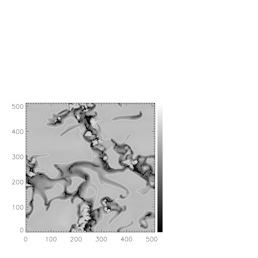
Figure 1: Temperature field at $t=5.03\times 10^{7}$ yr. The gray scale is logarithmic with darker tones at cooler regions. The maximum and minimum value are $1.77\times 10^{4}$ K and $95$ K, respectively. Superimposed contours show the upper (solid line) and lower (dashed line) limits of the unstable range. Note that much of the gas in the unstable regime is not directly associated with stellar activity.

The fiducial simulation reaches a stationary regime after $\sim 3.40\times 10^{7}$ yr. Figure 1 shows an image of the temperature field at $t=5.03\times 10^{7}$ yr. The contours show the upper (solid line) and lower (dashed line) boundary temperatures of the unstable range, $T_{4}$ and $T_{3}$. The small bright spots partially surrounded by cool dense gas are the stellar heating sites. For this field, fig. 2a shows the logarithmic, density-weighted temperature histogram (solid line) and the cumulative distribution (dotted line). The vertical lines indicate $T_{4}$ and $T_{3}$. Although the histogram is clearly bimodal, with peaks at temperatures just outside the unstable range, a roughly constant mass fraction per logarithmic temperature interval is seen to occur in the unstable regime. Given the large extension of the unstable range, the total mass in this range is $\sim 50$% of the mass in the simulation, with $\sim 25$% in both the cold and warm stable regimes. We have verified that the presence of the warm unstable gas is not due to diffusion. The temperature histogram does not change appreciably by decreasing the thermal diffusion term by a factor of 5 (fig. 2a; dashed and dashed-dotted lines). We also performed a simulation with all diffusivities reduced by factors $\sim 2$, and, although it cannot go beyond $t=3.26\times 10^{7}$ yr, the cumulative distribution of this simulation agrees to within a few percent with that of our fiducial run at that time throughout the temperature range (fig. 2b). Finally, we have also checked that the temperature PDF at a later time ($t=6.53\times 10^{7}$ yr) is virtually identical to that shown in fig. 2a, reassuring us that a statistically stationary state has been reached.

In order to understand these results, it is helpful to briefly describe the evolution of the simulation. As in Paper I, the initial density and velocity fluctuations generate filaments (recall the simulation is 2D), which can later fragment, redisperse, get stretched by the shear, collide with other filaments to either merge or disrupt, or any combination thereof. Most of the initial filaments do not form stars by themselves, except for those formed by the strongest initial fluctuations, which evolve in a manner similar to that described by Henebelle & Pérault (1999). Some filaments redisperse, apparently under the action of the other forces at play in the simulation, such as shear and tidal stresses, and magnetic pressure.

In most cases, the first SF events occur upon the collision of filaments, but subsequently SF auto-propagates, with new stars forming in the shells created by previous ones, although this self-propagation proceeds slowly due to the neglect of supernovae. The stellar heating in the simulation produces bubbles of warm gas that in general reach rather high temperatures (up to $\sim$ 15,000 K) while the stars are on. Individual stars hardly affect their parent cloud, but stars formed in “associations” create bubbles that merge with the warm, diffuse medium. After the stars turn off, these regions are left out of thermal equilibrium and, since they have also been evacuated to rather low densities ($\sim 0.2$–1 cm^-3), they require times $\sim 2$ Myr to return to thermal equilibrium in the warm “stable” range. At advanced evolutionary stages, the general impression is much more that of a temperature continuum than one of a two-phase medium. Regions in the thermally “unstable” range do not exhibit any systematic tendency to be systematically destroyed. This is most noticeable from watching the evolution of the contours at the “transition” temperatures. The contours bounding the unstable range in general do not appear to have a tendency to approach one another, but instead move in a typically advective fashion. This is in agreement with the nearly constant mass fraction ($\sim 50\%$) at unstable temperatures present in the simulation at various times. In addition, even though star formation self-propagates, many of the unstable regions in our simulation have never been under the influence of the stellar heating. This suggests that the other forces at play besides thermal pressure provide a net restoring force even in the unstable regime with respect to TI, in such a way that no abrupt phase transition occurs. We plan to investigate the detailed interplay between the various physical agents in a future paper.

It should be emphasized that the bimodal form of the histograms shown in fig. 2 does not imply that distinct phases must exist. It is sufficient that, under thermal equilibrium conditions, the equilibrium temperature $T_{\rm eq}$, plotted as a function of density, have extended nearly flat portions (“plateaus”) joined by short density intervals in which $T_{\rm eq}$ varies rapidly. Thus, even for a smoothly varying density distribution, the plateau temperatures will in general be more frequent than those at the intervals of rapid variation, with no need for a sharp (phase) transition from one temperature to the other. This will give a temperature PDF similar to those in fig. 2, with an excess at the plateau temperatures, but a non-zero population at intermediate temperatures.

4 Conclusions

In this Letter, we have shown that in our 2D simulations including the isobaric mode of TI, together with the magnetic field, self-gravity and energy injection mimicking that from OB-star ionizing radiation (but without supernovae), nearly half of the mass is at thermally unstable temperatures as shown by density-weighted temperature histograms. This is apparently partly the result of the other forces at play overwhelming the “crushing” drive of TI and restoring a “normal” (rather than reversed) effective pressure gradient, in such a way that there is no abrupt transition between the cold and warm gas, but rather there is a continuous temperature distribution. This is a different mechanism for maintaining the gas in the unstable range than the one in the models of Gerola et al. (1974), in which gas is heated and driven far from equilibrium at random times by stellar energy injection, creating a population of gas that traverses the “unstable” range as it cools. In this case, the simplified example given by McCray & Dalgarno (1972) suggests that the fraction of gas in this temperature range should depend on the star formation rate. In our simulations this cannot occur, as the gas is subject to global uniform background heating, so once it reaches the warm stable phase it has no tendency to cool further. But in the real ISM, in which the background heating is not uniform, but is strongest in the vicinity of stellar energy sources, this process is a real additional possibility.

The functional form of the cooling still affects the temperature PDF, producing peaks at the temperatures that would be stable under TI alone, but with a substantial fraction of the gas mass dwelling in the “unstable” range at all times. This result strengthens the view in Paper I that, under the presence of the many other physical ingredients relevant in the ISM, TI becomes a second-order effect, and suggests that dynamical processes should not be neglected in comprehensive models of the ISM.

It is important to note that, because of numerical limitations, our simulations do not include supernovae, and thus contain no hot gas. If supernovae were present, the cavities formed by them would reach temperatures $\sim 10^{6}$ K and expand much more than the stellar bubbles do here, due to the presence of the isochoric mode of TI above $\sim 10^{5}$ K. However, two lines of argument suggest that our results should hold even in the presence of supernovae. First, if the filling factor of the hot gas at the Galactic midplane is not too large ($\sim 20\%$; see, e.g., Ferrière 1998; Gazol-Patiño & Passot 1999; Avillez 2000), then our simulation can be thought of as representing the regions of the midplane not occupied by the hot gas. Second, the simulations of Korpi et al. (1999), which do include supernovae, albeit with an uncertain role of the isobaric mode of TI, give temperature histograms consistent in the cold and warm ranges with the ones presented in this paper. A definitive test on whether the presence of such hot gas would alter our conclusions will be provided by simulations including supernovae, which we intend to present, in 3D and using a different numerical scheme, in a future paper.

Figure 2: Density-weighted temperature histograms and cumulative distributions (divided by 10). In both panels, solid and dotted lines refer to the fiducial simulation shown in fig. 1, and dashed and dashed-dotted lines refer to comparison runs for testing convergence : Top (a), comparison with a run with thermal diffusion decreased by a factor of 5 at $t=5.03\times 10^{7}$ yr. Bottom (b), comparison with a run with all diffusivities decreased by a factor of $\sim 2$ at $t=2.04\times 10^{7}$ yr. In the top panel, in which a stationary state has been reached, the cumulative distribution shows that $\sim 50\%$ of the mass is in the unstable temperature range.

References

- (1) Avillez, M. A. 2000, MNRAS, 315,479
- (2) Ballesteros-Paredes, J., Vázquez-Semadeni, E., & Scalo, J. 1999, ApJ, 515, 286
- (3) Burkert, A., & Lin, D. N. C. 2000, ApJ, 537, 270
- (4) Cox, D. P. 1995, in “The physics of the Interstellar Medium and Intergalactic Medium”, ASP Conference Series, vol. 80 A. Ferrara, C. F. McKee, C. Heiles, & P. R. Shapiro (eds.), p.317
- (5) Dalgarno, A., & McCray, R. A. 1972, ARAA, 10, 375
- (6) Dickey, J. M., Salpeter, E. E., & Terzian, Y. 1977, ApJL, 211, L77
- (7) Elmegreen, B. G. 1991, ApJ, 378, 139
- (8) Elmegreen, B. G. 1994, ApJ, 433, 39
- (9) Elmegreen, B. G. 1997, ApJ, 477, 196
- (10) Ferrière, K. M. 1998, ApJ, 497, 759
- (11) Field, G. B., Goldsmith, D. W., & Habing, H. J. 1969, ApJ, 155, L149
- (12) Fitzpatrick, E. L., & Spitzer, L. 1997, ApJ, 475,623
- (13) Franco, J., & Carramiñana, A. 1999, Interstellar Turbulence, Proceedings of the 2nd Guillermo Haro Conference, Cambridge University Press
- (14) Gazol-Patiño, A., & Passot, T. 1999, ApJ, 518, 748
- (15) Gerola, H., Kafatos, M., & McCray, R. 1974, ApJ,189, 55
- (16) Heiles, C. 2001, ApJ 551, L105
- (17) Henebelle, P., & Pérault, M. 1999, A& A, 351, 309
- (18) Kornreich, P., & Scalo, J. 2000, ApJ, 531, 366
- (19) Kalberla, P. M. W., Schwartz, U. J., & Goss, W. M. 1985, A&A, 144, 27
- (20) Korpi, M. J., Brandenburg, A., Shukurov, A., Tuominen, I., & Nordlund, A. 1999, ApJ, 514, 99L
- (21) Kulkarni, S. R., & Heiles, C. 1987, in “Interstellar Processes”,ed. D. J. Hollenbach & H. A. Thronson. Reidel, Dordrecht, p.87
- (22) Lioure, A., & Chièze, J.-P. 1990, A&A, 235, 379
- (23) McCray, R., & Snow, T. P. Jr. 1979, ARA&A, 17, 213
- (24) McKee, C. F., & Ostriker, J. P. 1977, ApJ, 218, 148
- (25) Norman, C. A., & Ferrara, A. 1996, ApJ, 476, 280
- (26) Passot, T., Vázquez-Semadeni, E., & Pouquet, A. 1995, ApJ, 455, 536
- (27) Sánchez-Salcedo, F. J., Vázquez-Semadeni, E., & Gazol, A. 2001, in preparation
- (28) Scalo, J. M. 1987, in Interstellar Processes, ed. D. J. Hollenbach & H. A. Thronson, Dordrecht: Reidel), p. 349
- (29) Spitzer, L., & Fitzpatrick, E. L. 1995, ApJ, 445, 196
- (30) Vázquez-Semadeni, E., Passot, T., & Pouquet, A. 1995, ApJ 441, 702
- (31) Vázquez-Semadeni, E., Gazol, A., & Scalo, J. 2000a, ApJ, 540, 271 (Paper I)
- (32) Vázquez-Semadeni, E., Ostriker, E. C., Passot, T., Gammie, C., & Stone, J. 2000b in “Protostars & Planets IV”, ed. V. Mannings, A. Boss & S. Russell (Tucson: Univ. of Arizona Press), p. 3
- (33) Wolfire, M. G., Hollenbach, D., & McKee, C. F. 1995, ApJ, 443, 152