Decays of supernova neutrinos

Abstract

Supernova neutrinos could be well-suited for probing neutrino decay, since decay may be observed even for very small decay rates or coupling constants. We will introduce an effective operator framework for the combined description of neutrino decay and neutrino oscillations for supernova neutrinos, which can especially take into account two properties: One is the radially symmetric neutrino flux, allowing a decay product to be re-directed towards the observer even if the parent neutrino had a different original direction of propagation. The other is decoherence because of the long baselines for coherently produced neutrinos. We will demonstrate how to use this effective theory to calculate the time-dependent fluxes at the detector. In addition, we will show the implications of a Majoron-like decay model. As a result, we will demonstrate that for certain parameter values one may observe some effects which could also mimic signals similar to the ones expected from supernova models, making it in general harder to separate neutrino and supernova properties.

TUM-HEP-417/01

, ,

1 Introduction

Neutrino decay [1, 2] has been considered as an alternative to neutrino oscillations, especially for atmospheric [3, 4, 5, 6, 7, 8] and solar [3, 9, 10] neutrinos. Furthermore, sequential combinations of neutrino decay and neutrino oscillations have been studied (e.g., MSW-mediated solar neutrino decay [11, 10]), as well as a combined treatment [12]. Currently, one of the most favorable models for neutrino decay is to introduce an effective decay Lagrangian which couples the neutrino fields to a massless boson carrying lepton number, i.e., a complex scalar field or a Majoron field [13, 14, 15, 16]. One possibility for such a Lagrangian for the case of Majoron decay is

$$\mathcal{L}_{\rm int}=\underset{i\neq j}{\sum_{i}\sum_{j}}g_{ij}\overline{\nu_{j,L}^{c}}\nu_{i,L}J,$$ (1)

where the $\nu$’s are Majorana mass eigenfields and $J$ is a Majoron field. An interaction Lagrangian like this in general also implies coupling to active neutrino mass eigenstates. It was shown in Ref. [12] that interference effects, such as neutrino oscillations, are in principle possible before and after decay. There are several constraints to Majoron models, such as the exclusion of pure triplet models by the $Z^{0}$ width from LEP at CERN. However, fine-tuning or small triplet admixtures to singlet Majorons, as well as more sophisticated models have been proposed to circumvent this problem. For a more detailed discussion see, for example, Refs. [3, 4, 5]. Alternative neutrino decay models, such as the one mentioned in Ref. [17], proposing decay into more than one neutrino, have also been suggested. Nevertheless, since we are interested in fast neutrino decay possibilities, we will focus on models for decay of one neutrino into exactly one neutrino, which can be described by a Lagrangian similar to Eq. (1).

In this paper, we extend the effective operator formalism introduced in Ref.[12] to allow a time-dependent treatment of a supernova neutrino flux modified by neutrino decay and neutrino oscillations. In earlier works [18, 19, 20, 21], different aspects of supernova decay have been considered, which we want to combine into a general formalism. For the sake of the analytical accessibility, however, we have to make certain simplifications. Since we want to focus on the neutrino propagation in vacuum, we thus ignore matter effects as well as any other effect within the supernova. Nevertheless, as we will see, taking a superposition of mass eigenstates obtained from a numerical calculation within a supernova instead of an initial flavor state, can be done in a quite straightforward way in our formalism. Furthermore, we restrict ourselves to maximal one intermediate decay between production and detection or almost stable decay products. We are especially interested in possible modifications of the time dependence of a supernova neutrino signal. Therefore, we neglect other effects such as (cosmological and non-cosmological) redshift, asymmetries of the supernova flux, and spatial extension of the neutrino production region. However, we take into account dispersion by different traveling times of different mass eigenstates, since we want to study the physical effects of combining neutrino decay and neutrino oscillations. In addition, we incorporate that neutrino oscillations are affected by wave packet decoherence at long traveling distances if the neutrinos are coherently produced or leaving the supernova as superpositions of mass eigenstates at all. Since coherence of supernova neutrinos is still a question under discussion, we will a priori assume that supernova neutrinos are produced coherently as flavor states, but demonstrate how to obtain the incoherent limit thereafter. When taking into account the MSW effect, coherent emission can be achieved for appropriate parameter values violating the adiabaticity condition. In addition, for a three flavor neutrino scenario obtaining exactly one (pure) mass eigenstate emerging from the supernova is no longer valid. It may even be a superposition of two mass eigenstates, such that neutrino oscillations of supernova neutrinos (close to the supernova) cannot be excluded in general. Nevertheless, we will use the incoherent limit in most of our examples, since this is the most often assumed case.

We will cover three main topics in this paper: First, in Sec. 2 we will discuss the loss of coherence because of the long baselines and how this is modified by intermediate decays. Especially, we will use Majoron decay as an example for demonstration. Second, in Sec. 3, we will introduce a general formalism in order to be able to calculate time-dependent fluxes at the detector. It will also implement the coherence issues mentioned before. Since it will also work for decay models similar to Majoron decay, it will be treated somewhat decoupled from the initial discussion. Third, in the remaining sections, we will give some applications. In Sec. 4, we will demonstrate the time smearing of a source pulse by neutrino decay. Coming back to Majoron decay, in Sec. 5, we will take a closer look on the dynamics of a Majoron decay model and its implications. In the next section, Sec. 6, we will calculate the flux at the detector by also taking into account path lengths of different traveling paths. In addition, we will apply the results for Majoron decay we obtained in Sec. 5 in order to show the implications for this decay model. Finally, in Sec. 7, we will show the peculiarity of observing interference effects at the detector in the limit of quite large decay rates, even if the coherence lengths of the problem are much shorter than the baseline length. In almost all sections, we will use simple examples to visualize the indicated effects.

2 Coherence in neutrino oscillations and intermediate decays

The coherence length for neutrino oscillations is of the order $L^{\mathrm{coh}}\simeq{\sigma_{x}E^{2}\over|\Delta m^{2}|}$, where $\sigma_{x}$ is the width of a (Gaussian) wave packet [22, 23, 24, 25] or the wave packet overlap in the source or detector [26]. Thus, for typical values for supernova neutrinos coherence seems to be destroyed on their way to the Earth. However, since the decay may happen close to the source or detector, the distance between decay and production or detection may be much shorter than the coherence length. We will show that we may thus see coherent interference effects in certain cases, e.g., for very early decays. For this, we need to take into account that the wave packet width, which enters the coherence length, is in fact $\sigma_{x}^{2}=(\sigma_{x}^{P})^{2}+(\sigma_{x}^{D})^{2}$, i.e., the squared sum of the widths of the production $P$ and detection $D$ processes [23, 26]. One can visualize this by a detection process working on a much longer timescale than the production process. Therefore, though the wave packets may be well separated to a third observer at arrival, the detector will not be able to resolve them due to the time resolution of its detection process. However, neutrino oscillations may be washed out, e.g., for too large $\sigma_{x}^{D}>L^{\mathrm{osc}}$, since the detector then averages over the oscillation length. For supernova neutrinos, the width is because of $\sigma_{x}^{P}<10^{-11}\,\mathrm{m}\ll\sigma_{x}^{D}$ determined by the detection process only. Taking into account intermediate neutrino decays, the detection process $D$ corresponds to the decay process $X$ with its width $\sigma_{x}^{X}$. For Majoron decay of a relativistic mass eigenstate $i$ of energy $E$ into a mass eigenstate $j$, determined by the Majoron coupling constant $g_{ij}$, one can estimate the wave packet overlap by the decay rate $\Gamma_{ij}$ as

$$\sigma_{x}^{X}\simeq{1\over\Gamma_{ij}}=\mathcal{O}\left(\frac{E}{m_{i}m_{j}g_{ij}^{2}}\right),$$ (2)

where the exact value of $\Gamma_{ij}$ depends on the interaction Lagrangian [27]. Thus, the weaker the coupling constants $g_{ij}$ are, the slower is the process and the longer is the spatial extension of the wave packet. Especially, for $g_{ij}\rightarrow 0$ the wave packet width would become infinite. Nevertheless, we will see that neutrino oscillations are not possible in this limit because of another constraint to be satisfied. Equation (2) leads to a coherence length for supernova neutrinos

$$L^{\mathrm{coh},X}_{ab}\equiv\frac{4\sqrt{2}\sigma_{x}^{X}E^{2}}{\Delta m_{ab}^{2}}=\mathcal{O}\left(\frac{E^{3}}{m_{i}m_{j}\Delta m_{ab}^{2}g_{ij}^{2}}\right).$$ (3)

Here $\Delta m_{ab}^{2}$ is the mass squared difference of the neutrino oscillation considered (before or after decay). For instance, an incoming superposition of two mass eigenstates, oscillating in the flavor basis, say $\nu_{2}$ and $\nu_{3}$, may decay into an outgoing mass eigenstate, say $\nu_{1}$, by non-zero Majoron coupling constants $g_{31}$ and $g_{21}$. Then the index $i$ of the parent neutrino is $3$ or $2$, the index $j$ of the decay product is $1$, and the $\Delta m_{ab}^{2}$ considered is equal to $\Delta m_{32}^{2}$. From the last equation, Eq. (3), we see that especially for small coupling constants the coherence length can be quite long. However, in Refs.[23, 26], the upper bound

$$L^{\mathrm{coh}}_{ab}<\frac{16\pi^{2}E^{3}}{(\Delta m_{ab}^{2})^{2}}$$ (4)

was found for the coherence length, determined by the condition $\sigma_{x}<L^{\mathrm{osc}}$ necessary for neutrino oscillations not to be washed out by the spatial wave packet extension. Thus, this implies that $L^{\mathrm{coh}}<(10^{9}\sim 10^{19})\,\mathrm{m}$ for $\Delta m^{2}\simeq(10^{-5}\sim 1)\,\mathrm{eV}^{2}$, which is, in principle, much shorter than the typical distance of a supernova. In addition, in order to observe the oscillations before or after decay, this means for Majoron decay that

$$g_{ij}^{2}>\mathcal{O}\left(\frac{\Delta m_{ab}^{2}}{m_{i}m_{j}}\right)\quad\mathrm{or}\quad\alpha_{ij}\equiv\Gamma_{ij}E>\Delta m_{ab}^{2}=\mathcal{O}\left(\frac{\Delta m_{ab}^{2}}{\mathrm{eV^{2}}}\,\frac{\mathrm{GeV}}{\mathrm{km}}\right).$$ (5)

This is a finite lifetime condition similar to the one in Ref.[24] for the decaying muons used for neutrino production.

Since we want to obtain a treatment which is independent of the coherence discussion, we use the wave packet approach in Ref.[23] by assuming that coherence is destroyed by a factor $\exp[-(l/L^{\mathrm{coh}})^{2}]$. Here $L^{\mathrm{coh}}$ is given by Eq. (3) with the respective widths of the processes considered. In addition, model-dependent constraints may have to be applied to $L^{\mathrm{coh}}$. The following two cases will be discussed in this paper:

1. Coherence is lost before decay and detection, i.e., all coherence lengths involved in the problem are much shorter than the traveling distances between the interaction processes. In the models above, this can be easily achieved by violating Eq. (5).

2. All instable neutrinos have decayed before coherence is lost, which means that $\alpha L^{\mathrm{coh}}/E\gg 1$. Since for Majoron decay $\alpha$ as well as $L^{\mathrm{coh}}$ depends on the coupling constants, one can show that this condition together with Eq. (2) implies that $E^{2}/\Delta m_{ab}^{2}\gg 1$ in the wave packet model above applied to Majoron decay. This is always true for relativistic neutrinos and small $\Delta m^{2}$’s, such as often assumed for active neutrinos. In addition, constraints such as Eq. (5) may have to be satisfied for the neutrino oscillations considered.

Note that Secs. 4 and 6 are calculated for the first case. The last application, Sec. 7, corresponds to the second case.

3 The formalism

In this section, we will introduce the formalism used to calculate transition probabilities and fluxes. First, we will motivate the extension of the formalism in Ref.[12] by wave packet aspects and properties of point sources. Then, we will define the relevant operators, transition amplitudes, and fluxes. Finally, we will give certain limiting cases in order to be able to describe realistic scenarios by simplified formulas and to show that the formalism reduces to the one in Ref.[12] in the coherent limit.

3.1 Motivation

In Ref.[12], the combination of neutrino decay and neutrino oscillations was discussed for beams, but not for point sources. Baselines were assumed to be short enough such that the wave packets are still sufficiently overlapping at the position of decay and at the detector. Let us now generalize this with respect to the two above mentioned aspects.

3.1.1 Coherence and wave packets

In order to implement the loss of coherence by propagation over large distances, $L>L^{\mathrm{coh}}$, we follow the mentioned wave packet treatment of neutrino oscillations in Refs.[22, 23]. Therein it was noted that using wave packets leads to additional factors in the neutrino oscillation probabilities. The loss of coherence due to the spread and different mean velocities of sharply peaked wave packets is described by a factor $\exp[-(l/L^{\mathrm{coh},I}_{ab})^{2}]$ in the transition probabilities, where $L^{\mathrm{coh},I}_{ab}$ was defined in Eq. (3) and $\sigma_{x}^{I}$ is the spatial width of the wave packet determined by the production $P$ and detection $D$ processes $(\sigma_{x}^{I})^{2}=(\sigma_{x}^{P})^{2}+(\sigma_{x}^{D})^{2}$. In addition, a factor enters the neutrino oscillation formulas, which is equal to unity if the constraint in Eq. (4) holds [23]. Violating this constraint formally also can be achieved by making the coherence length very short.

Taking into account an intermediate decay process $X$ between production and detection, which corresponds to the detection process above, we expect a factor $\exp[-(l_{1}/L^{\mathrm{coh},I}_{ab})^{2}]$ in the transition probabilities, where $(\sigma_{x}^{I})^{2}=(\sigma_{x}^{P})^{2}+(\sigma_{x}^{X})^{2}\simeq(\sigma_{x}^{X})^{2}$ is the wave packet width for supernova neutrinos, $l_{1}$ is the distance from production to decay, and the indices $a$ and $b$ refer to the mass eigenstates before decay. This factor describes the loss of coherence in the in state of a decay process, i.e., interference effects caused by fixed relative phases in an incoming superposition of mass eigenstates are destroyed. Furthermore, in decay new wave packets are produced. This leads to additional factors $\exp[-(l_{2}/L^{\mathrm{coh},J}_{cd})^{2}]$ describing the coherence among the decay products $c$ and $d$ over the distance $l_{2}$ from decay to detection. In this case, the wave packet width $(\sigma_{x}^{J})^{2}=(\sigma_{x}^{X})^{2}+(\sigma_{x}^{D})^{2}$ is determined by the widths of the decay and detection processes. In Sec. 3.2, we will introduce an operator $\mathcal{S}$, which has the suggested properties.

3.1.2 Radially symmetric source fluxes and time dependence

The second aspect we want to integrate into our operator framework is time-dependent, radially symmetric source fluxes. We define $\Phi^{\mathrm{tot}}_{\alpha}(t)=dN_{\alpha}/dt$ to be the total source flux, i.e., the number of neutrinos of the flavor $\nu_{\alpha}$ emitted equally in any direction per time unit. Hence, $\int_{-\infty}^{\infty}\Phi^{\mathrm{tot}}_{\alpha}(t)dt=N_{\alpha}$ is the total number of neutrinos emitted by the source. In addition, let $\Phi^{D}_{\alpha\beta}(t)$ be the “flux” at the detector, i.e., the number of neutrinos per time unit produced as flavor $\nu_{\alpha}$ and detectable as flavor $\nu_{\beta}$. Since this flux knows about the produced flavor, it could also be calculated by the transition probability as well as the number of $\nu_{\beta}$ arriving per time unit at the detector, i.e., $\Phi^{D}_{\beta}$. Often the term flux is used for the function $\Phi^{D}_{\beta}$. However, in our notation $\Phi^{D}_{\beta}=\sum_{\alpha}\Phi^{D}_{\alpha\beta}$. Furthermore, we will split $\Phi^{D}_{\alpha\beta}(t)$ into $\Phi^{D,0}_{\alpha\beta}(t)$ and $\Phi^{D,1}_{\alpha\beta}(t)$, describing neutrino fluxes with no intermediate decays and one intermediate decay such as the transition probabilities $P_{\alpha\beta}^{0}$ and $P_{\alpha\beta}^{1}$ in Ref.[12]. These may either have to be added or not, depending on if the detector can distinguish undecayed particles from decay products (such as by energy resolution or spin) or not.

Since decaying neutrinos, which are initially traveling into directions other than that of the detector, can produce neutrinos which are re-directed towards the detector, we average for the calculation of $\Phi^{D,1}_{\alpha\beta}$ over all possible decay positions at which the secondary neutrinos may still arrive at the detector. Figure 1 defines the geometry of the problem, as well as the geometrical terms in the figure caption.

Figure 1: The geometry of a beam from the supernova SN to the detector D. The direct baseline has the length $L$, the baseline with one intermediate decay has the length $l_{1}+l_{2}$, where the neutrino travels $l_{1}$ before decay and $l_{2}$ after decay.

It is safe to assume that the detector is small compared with the distance to the decay position $\sqrt{D}\ll l_{2}$. Thus, we can use radial symmetry, introduce spherical coordinates, and reduce the spatial averaging to $\int d\cos\chi/2$. For $\Phi^{D,0}_{\alpha\beta}$ we only need to find the fraction of $\Phi_{\alpha}^{\mathrm{tot}}$ that can hit the detector by geometry, which is $\Delta(\cos\chi)_{D}/2$, i.e., the cosine range under which the detector is seen by the source.

Since a secondary neutrino produced by decay will arrive at the detector only with a certain probability due to kinematics, we introduce the function $\eta_{ij}(L,l_{1},l_{2},D)$ describing the fraction of decay products $j$ of parent neutrinos $i$ decaying at the position determined by $l_{1}$, $l_{2}$, and $L$, which will still arrive at the detector. It is given by

$$\eta_{ij}(L,l_{1},l_{2},D)\equiv\eta_{ij}(L,\chi,l_{1},D)\equiv{1\over\Gamma_{ij}}\int\limits_{\mathcal{D}}\left|{d\Gamma_{ij}\over d\cos\theta}\right|{1\over 2\pi}d\cos\theta d\phi,$$ (6)

where $\mathcal{D}$ denotes the surface of detection and $D$ its area, which is to be integrated over, and $\Gamma_{ij}$ is the total decay rate. For the description of the kinematics of mass eigenstates we will use the square root of this function, because amplitudes behave like square roots of particles [12]. We readily see from Fig. 1 that $l_{2}(L,\chi,l_{1})$ is determined by

$$l_{2}^{2}=L^{2}+l_{1}^{2}-2Ll_{1}\cos\chi,$$ (7)

i.e., we may, for example, choose $l_{1}$ and $l_{2}$ or $\chi$ and $l_{1}$ as sets of independent parameters. For Majoron models the redirection by decay is because of kinematics limited by a maximum angle $\theta_{\mathrm{max}}^{ij}$, where $\nu_{i}$ is the parent neutrino and $\nu_{j}$ the decay product. This angle can be shown to be very small for $\Delta m_{ij}^{2}$ not larger than $m_{i}^{2}$ or $m_{j}^{2}$ by many orders of magnitude and relativistic neutrinos, which is reasonable at least for active neutrinos with no extremely hierarchical mass spectrum. Generalizing this to any considered decay model, using $\chi$ and $l_{1}$ as independent parameters, and assuming the detection area $D$ to be small compared with the distance $l_{2}$, i.e., $\sqrt{D}\ll l_{2}$, we determine the parameter ranges from geometry for small angles to be

$$\chi \in [0,\,\theta_{\mathrm{max}}^{ij}],$$ (8)

$$l_{1} \in [0,\,l_{1,ij}^{\mathrm{max}}],\quad\mathrm{where}\ l_{1,ij}^{\mathrm{max}}\equiv L\left(1-{\chi\over\theta_{\mathrm{max}}^{ij}}\right).$$ (9)

Furthermore, we have to take care of time dispersion due to different traveling lengths. In general, $\Phi^{\mathrm{tot}}_{\alpha\beta}(t)\propto\Phi^{\mathrm{tot}}_{\alpha}(t-t_{1}^{(i)}-t_{2}^{(j)})$, where $t_{k}^{(a)}\simeq l_{k}[1+m_{a}^{2}/(2E^{2})]$ for relativistic mass eigenstates with mass $m_{a}$, $\nu_{i}$ is the mass eigenstate before decay, and $\nu_{j}$ is the one after decay. Thus, in order to integrate the time dependence of the source flux, we incorporate it at the time when the peaks of the wave packets arriving at the detector were emitted at the supernova. Traveling times are related to mass eigenstates, which are, at least within the coherence length, to be summed over coherently. However, the supernova produces flavor eigenstates. Thus, it will become useful to introduce the notion of an amplitude flux $\sqrt{\Phi^{\mathrm{tot}}}$, describing the flux of states instead of particles.

3.2 Operators, transition amplitudes, and fluxes

We will now define the relevant operators, transition amplitudes, and fluxes based on the discussions in the last section as well as in Ref.[12]. The decay rate is defined as $\alpha_{ij}\equiv\frac{m_{i}}{\tau^{0}_{ij}}$ for $i\rightarrow j$ decay, where $\tau^{0}_{ij}$ is the rest frame lifetime for that decay channel. Time dilation by the factor $\gamma_{i}=E_{i}/m_{i}$ implies that

$$\Gamma_{ij}^{\mathrm{observer}}=\Gamma_{ij}^{0}\gamma_{i}^{-1}={1\over\tau_{ij}^{0}}\frac{m_{i}}{E_{i}}={\alpha_{ij}\over E_{i}}.$$ (10)

The rate $\alpha_{i}\equiv\sum_{j}\alpha_{ij}$ is the overall decay rate of the state $i$, which means that $B_{ij}\equiv\frac{\alpha_{ij}}{\alpha_{i}}$ is the branching ratio for $i\rightarrow j$ decay. The energy $E_{i}$ of the mass eigenstate $i$ will be approximated by the mean energy $E$ of the produced flavor eigenstate if the energy corrections are of higher than first order. The operators will be defined in terms of effective creation $\hat{a}_{i}^{\dagger}$ and annihilation $\hat{a}_{i}$ operators operating on mass eigenstates [12].

Definition 1 (Disappearance operator)

$\mathcal{D}_{-}$ is the transition operator which is also often called “decay operator”. Effectively, it returns the amplitude for an undecayed state $i$ remaining undecayed after traveling a distance $l$ along the baseline $L$:

$$\mathcal{D}_{-}(l)=\sum\limits_{i}\exp\left(-\frac{\alpha_{i}t^{(i)}}{2E_{i}}\right)\hat{a}_{i}^{\dagger}\hat{a}_{i}\quad with\ t^{(i)}\simeq\left(1+{m_{i}^{2}\over 2E^{2}}\right)l.$$ (11)

Definition 2 (Appearance operator)

$\mathcal{D}_{+}$ is the differential transition operator, which destroys an in state and creates an out state in $[t_{1},t_{1}+dt_{1}]$ along the baseline $L$, i.e., a new state “appears”:

$$\mathcal{D}_{+}(L,l_{1},l_{2},D)=\underset{i\neq j}{\sum\limits_{i}\sum\limits_{j}}\sqrt{\frac{\alpha_{ij}}{E_{i}}}\ \sqrt{1+{m_{i}^{2}\over 2E^{2}}}\ \sqrt{\eta_{ij}(L,l_{1},l_{2},D)}\,\hat{a}_{j}^{\dagger}\hat{a}_{i}.$$ (12)

The probability density, which is the square of the amplitude, has to be integrated over $l_{1}$. Since $t^{(i)}\simeq(1+\frac{m_{i}^{2}}{2E^{2}})l$ for a mass eigenstate $\nu_{i}$, the transition amplitude, which is defined per time unit, needs to be transformed into an amplitude per length unit by the square root of this factor. Note that for a stationary problem the geometric function $\eta$ does not depend on traveling times.

Definition 3 (Propagation operator)

$\mathcal{E}^{k}$ is the operator propagating a state $\nu_{k}$ a distance $l$ along the baseline $L$:

$$\mathcal{E}^{k}(l)=\exp\left(-iE_{k}l\right)\hat{a}_{k}^{\dagger}\hat{a}_{k}.$$ (13)

The index $k$ will need to be summed over in the calculation of the flux, since time delays of different mass eigenstates will enter the (macroscopic) flux formula.

Definition 4 (Decoherence operator)

$\mathcal{S}^{I}(l,T)$ is the operator describing the loss of wave packet coherence of a state by traveling a distance $l$ along the baseline $L$:

$$\mathcal{S}^{I}(l,T)=\sum_{i}N^{I,i}\exp\left[-\frac{(l-v_{i}T)^{2}}{4(\sigma^{I}_{x})^{2}}\right]\,\hat{a}_{i}^{\dagger}a_{i}.$$ (14)

It turns out that this operator has the required properties leading to the factors postulated in Ref.[23] as well as in Sec. 3.1.1 in order to describe the loss of coherence for long baselines. The variable $T$ describes the wave packet distribution in time. It will be integrated over in the transition probability, since it is not measurable by the target process. In addition, $\sigma^{I}_{x}$ is the wave packet width of the composition $I$ of two processes (production, decay, or detection). Furthermore, $N^{I,i}$ is a normalization factor with

$$\int N^{I,i}N^{I,j}\exp\left[-\frac{(l-v_{i}T)^{2}+(l-v_{j}T)^{2}}{4(\sigma^{I}_{x})^{2}}\right]dT=\exp\left[-\left(\frac{l}{L^{\mathrm{coh},I}_{ij}}\right)^{2}\right].$$ (15)

Here the factor $\exp\{-(l-v_{a}T)^{2}/[4(\sigma^{I}_{x})^{2}]\}$ comes from the expansion of a sharply peaked wave packet, which can be written as $\Psi_{a}(L,T)=\exp[-iE_{a}T+ip_{a}L-(L-v_{a}T)^{2}/(4\sigma_{x}^{2})]$. In the definition of the propagation operator we ignored the factor $\exp(ip_{a}L)$, since it would only give rise to common phase factors as well as an additional, already mentioned factor, which is negligible for $\sigma_{x}\ll L^{\mathrm{osc}}$.

Definition 5 (Calculation of transition amplitudes)

The transition amplitude $A(\nu_{\alpha}\rightarrow\nu_{\beta})^{n}=A_{\alpha\beta}^{n}$ by exactly $n$ intermediate decays is for $n=0$

$$A_{\alpha\beta}^{0,i}=\langle\nu_{\beta}|\mathcal{E}^{i}(L)\mathcal{D}_{-}(L)\mathcal{S}^{PD}(L,T)|\nu_{\alpha}\rangle$$ (16)

and for $n=1$

$$A_{\alpha\beta}^{1,ij}=\langle\nu_{\beta}|\mathcal{E}^{j}(l_{2})\mathcal{D}_{-}(l_{2})\mathcal{S}^{XD}(l_{2},T)\mathcal{D}_{+}(L,l_{1},l_{2},D)\mathcal{E}^{i}(l_{1})\mathcal{D}_{-}(l_{1})\mathcal{S}^{PX}(l_{1},U)|\nu_{\alpha}\rangle.$$ (17)

The time variables $T$ and $U$ are to be integrated over in the transition probabilities, i.e., after taking the squares of the amplitudes. The indices $i$ and $j$, denoting the intermediate traveling mass eigenstates, are to be summed over in the calculation of the flux. Here $(\sigma_{x}^{AB})^{2}\equiv(\sigma_{x}^{A})^{2}+(\sigma_{x}^{B})^{2}$, where the label $P$ refers to the production process, $D$ to the detection process, and $X$ to the decay process.

Note that the order of $\mathcal{D}_{-}$, $\mathcal{S}$, and $\mathcal{E}$ is arbitrary, since it can be shown that these operators all commute.

Definition 6 (Calculation of fluxes)

The supernova neutrino fluxes $\Phi^{D,0}_{\alpha\beta}(t)$ (no intermediate decays) and $\Phi^{D,1}_{\alpha\beta}(t)$ (one intermediate decay) at the detector D are calculated as

$$\Phi^{D,0}_{\alpha\beta}(t) = \left|\sum\limits_{i}\sqrt{\Phi^{\mathrm{tot}}_{\alpha}(t-T^{(i)})}\,A_{\alpha\beta}^{0,i}\right|^{2}{\Delta(\cos\chi)_{D}\over 2},$$ (18)

$$\Phi^{D,1}_{\alpha\beta}(t) = \int\limits_{\cos\hat{\theta}_{\mathrm{max}}}^{1}\int\limits_{l_{1}=0}^{\hat{l}_{1}^{\mathrm{max}}}\left|\sum\limits_{i}\sum\limits_{j}\sqrt{\Phi^{\mathrm{tot}}_{\alpha}(t-t_{1}^{(i)}-t_{2}^{(j)})}\,A_{\alpha\beta}^{1,ij}\right|^{2}dl_{1}{d\cos\chi\over 2}$$ (19)

with $T^{(i)}\simeq\left(1+{m_{i}^{2}\over 2E^{2}}\right)L$, $t_{k}^{(i)}\simeq\left(1+{m_{i}^{2}\over 2E^{2}}\right)l_{k}$, $\hat{\theta}_{\mathrm{max}}=\max\theta_{\mathrm{max}}^{ij}$, and $\hat{l}_{1}^{\mathrm{max}}=\max l_{1,{ij}}^{\mathrm{max}}$.

In $\Phi^{D,1}_{\alpha\beta}$, we must integrate over the maximal possible range determined by the maximum of all $\theta_{\max}^{ij}$ and $l_{1,ij}^{\mathrm{max}}$, in order to cover the appropriate spatial region. If $(\chi,l_{1})$ is out of range, which may occur in some integrands, the function $\eta_{ij}$ in $\mathcal{D}_{+}$ will evaluate to zero.

3.3 Limiting cases

We now discuss some limiting cases. Most of them involve coherence limits and can also be combined with the limiting case in Sec. 3.3.3, i.e., neglecting different traveling path lengths.

3.3.1 Coherent wave packets

Let us assume that the wave packets are at all times coherent, i.e., $L\ll L^{\mathrm{coh}}$ for all coherence lengths involved in the problem. Hence, the decoherence operators $\mathcal{S}^{P}(l,T)$ will only give rise to factors of unity after the integration over time $T$, and hence, can be neglected. In addition, this implies that $l_{k}\simeq t_{k}$, i.e., we do not have to take into account differences between traveling times and propagation distances of different mass eigenstates. Finally, we assume that $\theta_{\mathrm{max}}^{ij}\simeq\theta_{\mathrm{max}}$ and $l^{\mathrm{max}}_{1,ij}\simeq l^{\mathrm{max}}_{1}$ to be independent of the indices $i$ and $j$, i.e., within the coherence length the mass eigenstates take approximately the same traveling paths. Therefore, we can pull the amplitude fluxes out of the summations over the intermediate traveling mass eigenstates, and redefine the propagation operators by absorbing the summations. In addition, we introduce probabilities instead of amplitudes. We then obtain the following expressions for the operators:

$$\mathcal{D}_{-}(l) = \sum\limits_{i}\exp\left(-\frac{\alpha_{i}l}{2E_{i}}\right)\hat{a}_{i}^{\dagger}\hat{a}_{i},$$ (20)

$$\mathcal{D}_{+}(L,l_{1},l_{2},D) = \underset{i\neq j}{\sum\limits_{i}\sum\limits_{j}}\sqrt{\frac{\alpha_{ij}}{E_{i}}}\ \sqrt{\eta_{ij}(L,l_{1},l_{2},D)}\,\hat{a}_{j}^{\dagger}\hat{a}_{i},$$ (21)

$$\mathcal{E}(l) = \sum\limits_{i}\exp\left(-iE_{i}l\right)\hat{a}_{i}^{\dagger}\hat{a}_{i}.$$ (22)

For the transition probabilities we have

$$P_{\alpha\beta}^{0} = \left|\left<\nu_{\beta}|\mathcal{E}(L)\mathcal{D}_{-}(L)|\nu_{\alpha}\right>\right|^{2},$$ (23)

$${dP_{\alpha\beta}^{1}\over dl_{1}} = \left|\left<\nu_{\beta}|\mathcal{E}(l_{2})\mathcal{D}_{-}(l_{2})\mathcal{D}_{+}(L,l_{1},l_{2},D)\mathcal{E}(l_{1})\mathcal{D}_{-}(l_{1})|\nu_{\alpha}\right>\right|^{2},$$ (24)

and for the fluxes we find

$$\Phi^{D,0}_{\alpha\beta}(t) = \Phi^{\mathrm{tot}}_{\alpha}(t-L){\Delta(\cos\chi)_{D}\over 2}P_{\alpha\beta}^{0},$$ (25)

$$\Phi^{D,1}_{\alpha\beta}(t) = \int\limits_{\cos\theta_{\mathrm{max}}}^{1}\int\limits_{l_{1}=0}^{l_{1}^{\mathrm{max}}}\Phi^{\mathrm{tot}}_{\alpha}(t-l_{1}-l_{2}){dP_{\alpha\beta}^{1}\over dl_{1}}dl_{1}{d\cos\chi\over 2}.$$ (26)

Therefore, the expressions found in this limit are very similar to the ones in Ref.[12], but adopted to point sources.

3.3.2 Incoherent wave packets

This limit corresponds to the first case mentioned in Sec. 2, i.e., loss of coherence between any two processes in the problem. Thus, we assume that $L,\,l_{1},\,l_{2}\gg L^{\mathrm{coh}}$ for all coherence lengths in the problem. Hence, the operators $\mathcal{S}^{I}(l,T)$ will give rise to factors $\exp[-(l/L^{\mathrm{coh},I}_{ij})^{2}]\rightarrow\delta_{ij}$ after the integration over the time $T$. It can be shown by application of the operators that this corresponds to incoherent summation over the intermediate traveling states, i.e., $|\sum_{ij}f_{ij}|^{2}\equiv\sum_{ij}|f_{ij}|^{2}$ in this limit. Therefore, we can square the amplitude fluxes, put the summations in front of the integrations in $\Phi^{D,1}_{\alpha\beta}$, and contract the integration limits back to the appropriate regions. We then may define transition probabilities

$$P_{\alpha\beta}^{0,i} = \left|\left<\nu_{\beta}|\nu_{i}\right>\right|^{2}\left|\left<\nu_{i}|\mathcal{D}_{-}(L)|\nu_{i}\right>\right|^{2}\left|\left<\nu_{i}|\nu_{\alpha}\right>\right|^{2},$$ (27)

$${dP_{\alpha\beta}^{1,ij}\over dl_{1}} = \left|\left<\nu_{\beta}|\nu_{j}\right>\right|^{2}\left|\left<\nu_{j}|\mathcal{D}_{-}(l_{2})\mathcal{D}_{+}(L,l_{1},l_{2})\mathcal{D}_{-}(l_{1})|\nu_{i}\right>\right|^{2}\left|\left<\nu_{i}|\nu_{\alpha}\right>\right|^{2},$$ (28)

and fluxes

$$\Phi^{D,0}_{\alpha\beta}(t) = \sum\limits_{i}\Phi^{\mathrm{tot}}_{\alpha}(t-T^{(i)})\,P_{\alpha\beta}^{0,i}{\Delta(\cos\chi)_{D}\over 2},$$ (29)

$$\Phi^{D,1}_{\alpha\beta}(t) = \sum\limits_{i}\sum\limits_{j}\int\limits_{\cos\theta_{\mathrm{max}}^{ij}}^{1}\int\limits_{l_{1}=0}^{l_{1,ij}^{\mathrm{max}}}\Phi^{\mathrm{tot}}_{\alpha}(t-t_{1}^{(i)}-t_{2}^{(j)})\,{dP_{\alpha\beta}^{1,ij}\over dl_{1}}dl_{1}{d\cos\chi\over 2}$$ (30)

with $T^{(i)}\simeq\left(1+{m_{i}^{2}\over 2E^{2}}\right)L$ and $t_{k}^{(i)}\simeq\left(1+{m_{i}^{2}\over 2E^{2}}\right)l_{k}$. Thus, $\mathcal{S}$ splits up the formulas for the transition amplitudes such that neutrino oscillations vanish.

3.3.3 Neglecting time delays by different traveling paths

Time delays due to different path lengths can be neglected when they are small compared with time delays by different masses. The fraction of the initial flux arriving at the detector is $D/4\pi L^{2}$, since the total flux through any sphere around the point source is equal by symmetry. This is, in principle, not changed for decays from one mass eigenstate into another, since the overall number of neutrinos arriving at the detector is unchanged. Nevertheless, the relative arrival times may differ for different path lengths. The time delay due to different path lengths $\Delta t_{1,ij}$ for mass eigenstates $\nu_{i}$ and $\nu_{j}$, propagating before and after decay, respectively, can for small $\theta_{\mathrm{max}}^{ij}$ be approximated by $\Delta t_{1,ij}<\Delta t_{1,ij}^{\mathrm{max}}\simeq L(\theta_{\mathrm{max}}^{ij})^{2}/2$ from geometry. For this small time interval, delays by different masses can be ignored as second order effects. In order to have the limiting case discussed here, it needs to be much smaller than the time delay by different masses $\Delta t_{2,ij}=\Delta m_{ij}^{2}L/(2E^{2})$. Therefore, for $\theta_{\mathrm{max}}^{ij}\ll\sqrt{\Delta m_{ij}^{2}}/E$ effects of different path lengths can be neglected. In fact, it can be shown that this is equivalent to $\Delta m_{ij}^{2}\ll m^{2}_{j}$ in the case of Majoron decay. However, the time delay caused by different path lengths may still be measurable if the absolute value of $\Delta t_{1}$ is longer than the time resolution of the detector.

Since we are ignoring traveling times due to different paths and since the total number of arriving particles is not changed by decay, we can implement this limiting case in the geometrical function $\eta$, describing the fraction of secondary neutrinos hitting the detector, as

$$\eta(L,\chi,l_{1},D)=\frac{D}{4\pi L^{2}}\,4\delta(1-\cos\chi).$$ (31)

Thus, the secondary neutrinos are peaked in the forward direction and for any $x<1$ the integral $\int_{x}^{1}\,\eta\,d\cos\chi/2=D/(4\pi L^{2})$ gives the required fraction independent of the indices $i$ and $j$. Note that this definition of $\eta$ corresponds to a forward peaked differential decay rate $d\Gamma_{ij}/d\cos\theta\propto\delta(1-\cos\theta)$ in Eq. (6). However, it is not exactly identical due to re-direction effects. Nevertheless, a distribution of the differential decay rate, which is sharply peaked into the forward direction, gives an effective $\tilde{\theta}_{\mathrm{max}}^{ij}\ll\theta_{\mathrm{max}}^{ij}$. Then, for the case of $\tilde{\theta}_{\mathrm{max}}^{ij}\ll\sqrt{\Delta m_{ij}^{2}}/E$, we have this limit again. We will introduce in Sec. 5 an $\eta$-function which corresponds to this case.

In order to incorporate the new $\eta$-function in this limiting case, we only need to re-define one operator:

$$\mathcal{D}_{+}=\underset{i\neq j}{\sum\limits_{i}\sum\limits_{j}}\sqrt{\frac{\alpha_{ij}}{E_{i}}}\ \sqrt{1+{m_{i}^{2}\over 2E^{2}}}\,\hat{a}_{j}^{\dagger}\hat{a}_{i},$$ (32)

In addition, we need to take into account that $l_{2}=L-l_{1}$ in the evaluation of the $\chi$-integration over the $\delta$-distribution in the $\eta$-function. Finally, we obtain for the fluxes for $l_{1}\equiv l$

$$\Phi^{D,0}_{\alpha\beta}(t) = \left|\sum\limits_{i}\sqrt{\Phi^{\mathrm{tot}}_{\alpha}(t-T^{(i)})}\,A_{\alpha\beta}^{0,i}\right|^{2}\,{D\over 4\pi L^{2}},$$ (33)

$$\Phi^{D,1}_{\alpha\beta}(t) = \int\limits_{l=0}^{L}\left|\sum\limits_{i}\sum\limits_{j}\sqrt{\Phi^{\mathrm{tot}}_{\alpha}(t-t_{1}^{(i)}-t_{2}^{(j)})}\,A_{\alpha\beta}^{1,ij}\right|^{2}dl_{1}\,{D\over 4\pi L^{2}}$$ (34)

with $T^{(i)}\simeq\left(1+{m_{i}^{2}\over 2E^{2}}\right)L$, $t_{1}^{(i)}\simeq\left(1+{m_{i}^{2}\over 2E^{2}}\right)l$, and $t_{2}^{(j)}\simeq\left(1+{m_{j}^{2}\over 2E^{2}}\right)(L-l)$. Simultaneous application of the incoherent limit yields in addition formulas adjusted to the last limiting case in a straightforward way.

3.3.4 Decay before loss of coherence

In this limit, we treat the second case mentioned in Sec. 2, i.e., decay rates large enough such that all of the neutrinos decay before coherence is lost. If we assume that $L\gg L^{\mathrm{coh}}$, the wave packets of undecayed states will loose coherence before detection, i.e., $\Phi^{D,0}_{\alpha\beta}$ can be calculated as in Sec. 3.3.2. For very early decays, i.e., $\alpha\gg E/L^{\mathrm{coh}}$, the distance $l_{2}$ is much longer than the corresponding coherence length, whereas $l_{1}$ is shorter. In this case, all initial neutrinos have decayed before $l_{1}$ approaches the coherence length, which also means that $\Phi^{D,0}_{\alpha\beta}\simeq 0$. Furthermore, since $L\gg L^{\mathrm{coh}}$, the decay products will loose coherence before detection. In order to understand what may happen in this limiting case, we assume interference between different decay channels, i.e., simultaneous couplings to the decay products, such as by Majoron coupling constants $g_{ik}>0$ and $g_{jk}>0$ for different indices $i$, $j$, and $k$. Then, the relative phase of the states in the incoming superposition depends on the decay position. In addition, the arrival time depends on the decay position, because the mass eigenstates travel with different velocities before and after decay. We expect to observe the most interesting interference effects for $\Delta m^{2}\simeq\alpha$. For fast oscillations, i.e., $\Delta m^{2}\gg\alpha$, interference effects will be washed out by averaging over the different decay positions. For slow oscillations, i.e., $\Delta m^{2}\ll\alpha$, all particles will still have the initial relative phase at the decay position, eliminating any oscillating effect.

In order to calculate the transition flux $\Phi^{D,1}_{\alpha\beta}$, we combine the formulas in Secs. 3.3.1 (before decay) and 3.3.2 (after decay). We define

$$\bar{t}_{1}\equiv\left(1+\frac{\overline{m^{2}}}{2E^{2}}\right)l_{1}\quad\mathrm{with}\quad\overline{m^{2}}\equiv\frac{1}{N}\sum\limits_{i=1}^{N}m_{i}^{2},$$ (35)

where the mass square average is to be taken over the $N$ mass eigenstates oscillating before decay. Since this mean traveling time will only enter in the total source flux and $l_{1}$ is assumed to be quite short, this is certainly a reasonable approximation for the source flux not changing too much on timescales of the order $\Delta m^{2}l_{1}/(2E^{2})$. In addition, we assume $\theta_{\mathrm{max}}^{ij}\simeq\theta_{\mathrm{max}}^{j}$ and $l_{1,ij}^{\mathrm{max}}\simeq l_{1,j}^{\mathrm{max}}$ to depend only on the decay products (the incoming wave packets are coherent). Eventually, this yields

$${dP_{\alpha\beta}^{1,j}\over dl_{1}} = \underbrace{\Big{|}\langle\nu_{\beta}|\nu_{j}\rangle\Big{|}^{2}\Big{|}\langle\nu_{j}|\mathcal{D}_{-}(l_{2})}_{\mathrm{incoherent}}\,\underbrace{\mathcal{D}_{+}(L,l_{1},l_{2})\mathcal{E}(l_{1})\mathcal{D}_{-}(l_{1})|\nu_{\alpha}\rangle\Big{|}^{2}}_{\mathrm{coherent}},$$ (36)

$$\Phi^{D,1}_{\alpha\beta}(t) = \sum\limits_{j}\int\limits_{\cos\theta_{\mathrm{max}}^{j}}^{1}\int\limits_{l_{1}=0}^{l_{1,j}^{\mathrm{max}}}\Phi^{\mathrm{tot}}_{\alpha}(t-\bar{t}_{1}-t_{2}^{(j)})\,{dP_{\alpha\beta}^{1,j}\over dl_{1}}dl_{1}{d\cos\chi\over 2},$$ (37)

with the operators from the coherent part as given in Sec. 3.3.1.

4 Incoherent mass dispersion

In this section, we will demonstrate for the limiting case of incoherent propagation how mass dispersion can be caused by decay even if we ignore different traveling path lengths. This is done by simultaneous application of the limits in Secs. 3.3.2 and 3.3.3. We will show that it is possible to observe a time dispersion by decay even for a pulsed source flux. Thus, we assume that $\Phi^{\mathrm{tot}}_{\alpha}(t)=N_{\alpha}\,\delta(t+L)$ which describes a neutrino pulsed produced at $t=-L$, where $N_{\alpha}$ is the total number of neutrinos of flavor $\nu_{\alpha}$ emitted by the supernova. In this case, it will be possible to detect massless neutrinos at $t=0$ and massive neutrinos delayed by $\Delta t^{(i)}={m_{i}^{2}l\over 2E^{2}}$. Decay leads to a time dispersion, since a mass eigenstates travels with a different velocity before and after decay. Its arrival time depends therefore on the decay position.

Combing the limiting cases in Secs. 3.3.2 and 3.3.3 as well as applying the transition probabilities and operators, we obtain for $\Phi_{\alpha\beta}^{D,1}$

$$\Phi^{D,1}_{\alpha\beta}(t) = \underset{i\neq j}{\sum\limits_{i}\sum\limits_{j}}\int\limits_{l=0}^{L}\frac{N_{\alpha}D}{4\pi L^{2}}\delta\left(t-\left(1+{m_{i}^{2}\over 2E^{2}}\right)l-\left(1+{m_{j}^{2}\over 2E^{2}}\right)(L-l)+L\right)$$ (38)

$$\times |U_{\alpha i}|^{2}|U_{\beta j}|^{2}e^{-{\alpha_{j}\over E}(L-l)\left(1+{m_{j}^{2}\over 2E^{2}}\right)}{\alpha_{ij}\over E}e^{-{\alpha_{i}\over E}l\left(1+{m_{i}^{2}\over 2E^{2}}\right)}\left(1+{m_{i}^{2}\over 2E^{2}}\right)dl.$$

The $\delta$-distribution in this formula, describing the neutrino pulse, implies that

$$t={\Delta m_{ij}^{2}\over 2E^{2}}l+{m_{j}^{2}\over 2E^{2}}L$$ (39)

or, for $m_{i}\neq m_{j}$,

$$l={2E^{2}\over\Delta m_{ij}^{2}}\left(t-{m_{j}^{2}\over 2E^{2}}L\right).$$ (40)

The condition $0\leq l\leq L$, for which the $\delta$-distribution evaluates to a non-zero value by the integration, is then equivalent to

$${m_{j}^{2}\over 2E^{2}}L\leq t_{ij}\leq{m_{i}^{2}\over 2E^{2}}L.$$ (41)

Thus, the signal arrives at the detector between the signals of the undecayed heavy mass eigenstate and the light one produced by the intermediate decay. Note that the allowed time interval depends on the indices $i$ and $j$. In addition, we need to take into account that $\delta\left(f(l)\right)=\delta(l-a)/|f^{\prime}(a)|_{f(a)=0}=2E^{2}/\Delta m_{ij}^{2}\delta(l-a)$ with $a$ equal to $l$ as given in Eq. (40). Finally, integrating over $l$ leads to

$$\Phi^{D,1}_{\alpha\beta}(t) = \underset{i\neq j}{\sum\limits_{i}\sum\limits_{j}}\frac{N_{\alpha}D}{4\pi L^{2}}|U_{\alpha i}|^{2}|U_{\beta j}|^{2}{2E\alpha_{ij}\over\Delta m_{ij}^{2}}\left(1+{m_{i}^{2}\over 2E^{2}}\right)e^{-{\alpha_{j}\over E}L\left(1+{m_{j}^{2}\over 2E^{2}}\right)}$$

$$\times \exp\left\{\left[\alpha_{j}\left(1+{m_{j}^{2}\over 2E^{2}}\right)-\alpha_{i}\left(1+{m_{i}^{2}\over 2E^{2}}\right)\right]{2E\over\Delta m_{ij}^{2}}\left(t-{m_{j}^{2}\over 2E^{2}}L\right)\right\}.$$

In the limit of stable decay products, i.e., $\alpha_{j}\rightarrow 0$, and by ignoring corrections of the order $m^{2}/E^{2}$ to the signal height, this reduces to

$$\Phi^{D,1}_{\alpha\beta}(t)=\underset{i\neq j}{\sum\limits_{i}\sum\limits_{j}}\frac{N_{\alpha}D}{4\pi L^{2}}|U_{\alpha i}|^{2}|U_{\beta j}|^{2}{2E\alpha_{ij}\over\Delta m_{ij}^{2}}\exp\left[-\alpha_{i}{2E\over\Delta m_{ij}^{2}}\left(t-{m_{j}^{2}\over 2E^{2}}L\right)\right].$$ (43)

Thus, the flux pulse of the source is smeared out to an exponentially dropping signal at the detector. Here the allowed range for $t_{ij}$ depends on the mass eigenstates $i$ and $j$ and is given in Eq. (41). One can immediately see that the smearing is determined by the coefficient $\alpha_{i}E/\Delta m_{ij}^{2}$ in the exponential. We obtain maximal smearing for small $\alpha_{i}E/\Delta m_{ij}^{2}$, i.e., small $\alpha_{i}$’s or large $\Delta m_{ij}^{2}$’s. A numerical analysis for typical values of $\Delta m_{ij}^{2}$, $E$, and $L$ shows that the $\alpha_{ij}$’s, and the Majoron coupling constants $g_{ij}$’s, respectively, can be far below any currently assumed upper limit for observing exponential dropping of this function (for constraints on the $g_{ij}$’s, see Refs.[29, 30, 31, 32]). However, if $\alpha_{i}$ is too small, the factor $\alpha_{ij}$ will suppress the term $\Phi^{D,1}_{\alpha\beta}$ completely.

We illustrate the effect for the following three-neutrino scenario: Maximal mixing, i.e., $|\nu_{\alpha}\rangle={1\over\sqrt{3}}|\nu_{1}\rangle+{1\over\sqrt{3}}|\nu_{2}\rangle+{1\over\sqrt{3}}|\nu_{3}\rangle$ ($\theta_{12}=\theta_{13}=\theta_{23}=45^{\circ}$ and $\delta_{CP}=0$), decay of $\nu_{3}$ into $\nu_{2}$ or $\nu_{1}$ only, i.e., $\alpha_{32}=\alpha_{31}=10^{-21}\,\mathrm{GeV\,km^{-1}}$, $E=10\,\mathrm{MeV}$, $L=10^{22}\,\mathrm{m}\simeq 32\,\mathrm{kpc}$, $N_{\alpha}=9\cdot 10^{5}\,(4\pi L^{2})/D$, $m_{3}=4\,\mathrm{eV}$, $m_{2}=2\,\mathrm{eV}$, and $m_{1}=1\,\mathrm{eV}$, which means that $\Delta m_{32}^{2}=12\,\mathrm{eV}^{2}$ and $\Delta m_{21}^{2}=3\,\mathrm{eV}^{2}$. We can use Eqs. (18) and (43) to evaluate $\Phi^{D,0}_{\alpha e}$ and $\Phi^{D,1}_{\alpha e}$, where the sums are split up in order to see the different signals from different mass eigenstates. Figure 2 shows the separated signals of the decay products $\Phi^{D,1}_{\alpha e}$ as well as the ones from the undecayed particles $\Phi^{D,0}_{\alpha e}$.

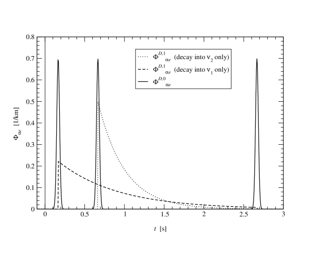
Figure 2: The (separated) signals of the decay products $\Phi^{D,1}_{\alpha e}$ and those of the undecayed particles $\Phi^{D,0}_{\alpha e}$ for the scenario constructed in the text. The $\delta$-distributions in $\Phi^{D,0}_{\alpha e}$ are plotted as Gaussian signals, where the leftmost refers to the lightest and the rightmost to the heaviest mass eigenstate. The vertical line at $t=0$ indicates the reference time when massless neutrinos would arrive.

It has been observed [33] that the SN1987A data can be reasonably fit to a decaying exponential with time constant $\tau\simeq 3\,\mathrm{s}$. Figure 2 indicates that we can easily find parameter sets in order to have an effect with a similar time dependence. However, for the currently assumed parameter values for active neutrinos, as shown in Fig. 3, the timescale of this effect would be rather short.

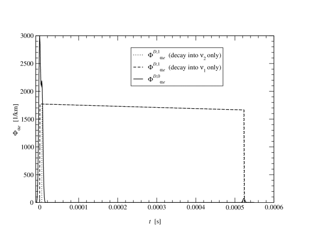
Figure 3: The signals of the decay products $\Phi^{D,1}_{\alpha e}$ and those of the undecayed particles $\Phi^{D,0}_{\alpha e}$ for the scenario with the parameter values $\Delta m_{32}^{2}=2.5\cdot 10^{-3}\,\mathrm{eV}^{2}$, $\Delta m_{21}^{2}=3.65\cdot 10^{-5}\,\mathrm{eV}^{2}$, $m_{1}=10^{-5}\,\mathrm{eV}$ (absolute neutrino mass value needed here), $\theta_{12}=\theta_{23}=45^{\circ}$ (bimaximal mixing), $\theta_{13}=5^{\circ}$, and $\delta_{CP}=0$. The other parameter values are the same as for Fig. 2. Note that $\alpha$ can be equal to $\mu$ or $\tau$. For $\alpha=e$ the result will be different, since the mixing is not trimaximal anymore as in Fig. 2. Furthermore, note that the scale of the fluxes is not applicable to the $\delta$-fluxes illustrated as peaked signals, but the heights of these peaks reflect their relative values.

In addition, the two different decay channels could, mainly due to the small $\Delta m_{21}^{2}$, not be resolved anymore. Thus, in order to be able to identify all relevant individual effects in the plots, we will further on choose parameter values which amplify these effects more clearly, but which are not the values currently favored by data. There are basically two arguments supporting this point of view. First, the best-fit parameters may change when making global fits with neutrino decay included, and therefore, the mass squared differences may become larger. Second, more recently, other models being relevant for this sort of discussion have been introduced, such as in Ref. [34], in which the decay of a light sterile neutrino into active neutrinos was proposed. In this case, the relevant mass squared differences could again be rather large. Such light sterile neutrinos could be produced by oscillated supernova neutrinos close to or within the supernova.

5 Dynamics of Majoron decay

Let us now give an approximation for the function $\eta_{ij}(L,\chi,l_{1},D)$ defined in Eq. (6) for Majoron decay of relativistic neutrinos. It describes the fraction of decay products arriving at the detector for decay at $(\chi,l_{1})$ (cf., Fig. 1). Since only a small fraction of neutrinos will decay close to the detector, we can assume that

$$L\geq l_{2}\gg\sqrt{D}/\theta_{\mathrm{max}}^{ij},$$ (44)

where $\theta_{\mathrm{max}}^{ij}$ is given by [12]

$$\theta_{\mathrm{max}}^{ij}={m_{j}\over 2E_{i}}\left(x^{2}-1\right),\qquad x\equiv{m_{i}\over m_{j}}.$$ (45)

Here the index $i$ refers to the parent neutrino and $j$ to the decay product. Hence, we can treat the detector as a point target and approximate Eq. (6) by

$$\eta_{ij}(L,\chi,l_{1},D)={1\over\Gamma_{ij}}\left|{d\Gamma_{ij}\over d\cos\theta}\right|_{(\cos\theta)_{D}}{1\over 2\pi}\Delta\Omega={1\over\Gamma_{ij}}\left|{d\Gamma_{ij}\over d\cos\theta}\right|_{(\cos\theta)_{D}}{D\over 2\pi l_{2}^{2}}$$ (46)

with $l_{2}$ given by Eq. (7). From

$$E_{i}-E_{j}=|\mathbf{p}_{i}-\mathbf{p}_{j}|=\sqrt{|\mathbf{p}_{i}|^{2}+|\mathbf{p}_{j}|^{2}-2|\mathbf{p}_{i}||\mathbf{p}_{j}|\cos\theta},$$ (47)

which determines the kinematics of the process, we find for small $\theta$ two energies $E_{j}$ corresponding to one angle $\theta$

$$E_{j}^{\pm}(\theta)=\frac{E_{i}(1+x^{2})}{2\left({E_{i}^{2}\theta^{2}\over m_{j}^{2}}+x^{2}\right)}\left[1\pm\sqrt{1-4\frac{{E_{i}^{2}\theta^{2}\over m_{j}^{2}}+x^{2}}{(1+x^{2})^{2}}}\right].$$ (48)

Equation (46) can be written as

$$\eta_{ij}(L,\chi,l_{1},D)={1\over\Gamma_{ij}}{D\over 2\pi l_{2}^{2}}\left\{\left|{d\Gamma_{ij}\over dE_{j}}\right|_{E_{j}^{+}}\left|{dE_{j}\over d\cos\theta}\right|_{E_{j}^{+}}+\left|{d\Gamma_{ij}\over dE_{j}}\right|_{E_{j}^{-}}\left|{dE_{j}\over d\cos\theta}\right|_{E_{j}^{-}}\right\}.$$ (49)

The differential and total decay rates in this equation are for (pseudoscalar or scalar) Yukawa couplings in the Lagrangian for decay into neutrinos or antineutrinos given in Refs.[12, 27], respectively, for the Lagrangians introduced there. From Eq. (47) we read off

$$\left|{dE_{j}\over d\cos\theta}\right|_{E_{j}^{\pm}}=\frac{|\mathbf{p}_{i}||\mathbf{p}_{j}|}{|E_{i}-E_{j}|}\simeq\frac{E_{i}}{\left|{E_{i}\over E_{j}}-1\right|}.$$ (50)

Since we use $\chi$ and $l_{1}$ as independent parameters, we need to express $\theta$ in terms of $\chi$. To first approximation for small angles, which is reasonable for a small $\theta_{\mathrm{max}}^{ij}$, we find from geometry

$$\theta\simeq\left(1+{l_{1}\over l_{2}}\right)\chi\simeq\left(1+\frac{l_{1}}{L-l_{1}}\right)\chi.$$ (51)

Now $\eta$ can be evaluated numerically and is plotted in Figs. 4, 5, and 6 for (pseudoscalar or scalar) Yukawa couplings in the Lagrangian and decay into neutrinos and antineutrinos.

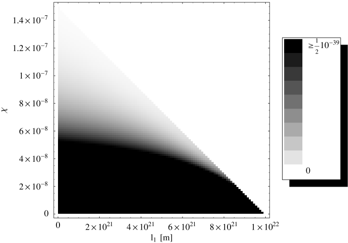
Figure 4: Density plot with a linear shading scale of the function $\eta_{ij}(\chi,l_{1})$ for pseudoscalar Yukawa couplings in the Lagrangian (decay into neutrinos). Here $D=10000\,\mathrm{m}^{2}$, $L=10^{22}\,\mathrm{m}\simeq 32\,\mathrm{kpc}$, $E_{i}=E=10\,\mathrm{MeV}$, $m_{i}=2\,\mathrm{eV}$, and $m_{j}=1\,\mathrm{eV}$. For the geometry of the problem, see Fig. 1.

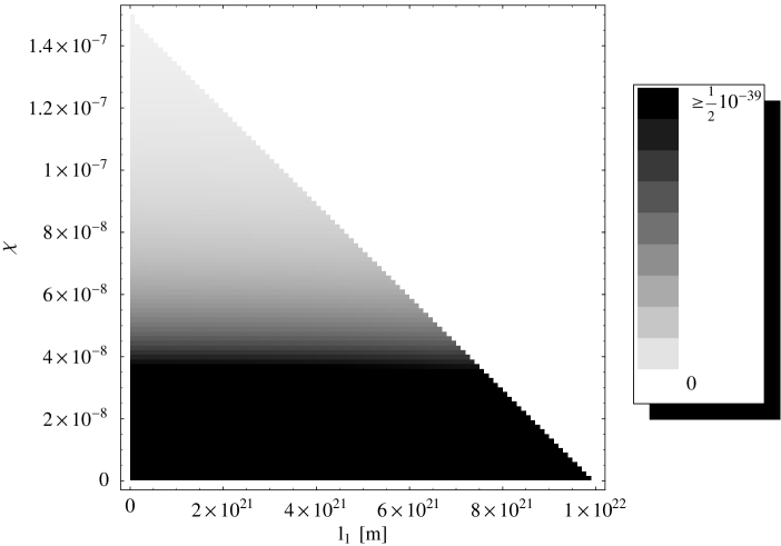
Figure 5: Density plot with a linear shading scale of the function $\eta_{ij}(\chi,l_{1})$ for scalar Yukawa couplings in the Lagrangian (decay into neutrinos). Here $D=10000\,\mathrm{m}^{2}$, $L=10^{22}\,\mathrm{m}\simeq 32\,\mathrm{kpc}$, $E_{i}=E=10\,\mathrm{MeV}$, $m_{i}=2\,\mathrm{eV}$, and $m_{j}=1\,\mathrm{eV}$. For the geometry of the problem, see Fig. 1.

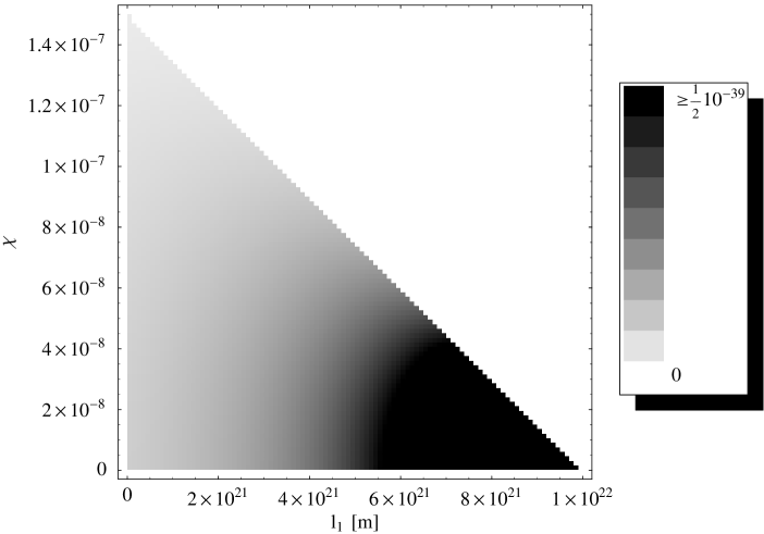
Figure 6: Density plot with a linear shading scale of the function $\eta_{ij}(\chi,l_{1})$ for pseudoscalar or scalar Yukawa couplings in the Lagrangian (decay into antineutrinos). Here $D=10000\,\mathrm{m}^{2}$, $L=10^{22}\,\mathrm{m}\simeq 32\,\mathrm{kpc}$, $E_{i}=E=10\,\mathrm{MeV}$, $m_{i}=2\,\mathrm{eV}$, and $m_{j}=1\,\mathrm{eV}$. For the geometry of the problem, see Fig. 1.

Note that the parameter ranges determined in Eqs. (8) and (9) imply that $\eta$ evaluates to zero, i.e., nothing arrives at the detector if the parameter set lies within the upper-right triangle over the diagonal. In this case, the secondary neutrino cannot be re-directed towards the detector anymore for kinematical reasons. The plot for antineutrinos shows, in comparison to the neutrino plots, that the direct path ($\chi=0$) is suppressed for small $l_{1}$, because of a spin flip. For Yukawa scalar couplings $\eta$ turns out to be quite independent of the angle $\chi$. In all cases, we can expect heavy suppression for too large $\chi$.

The magnitude of $\eta$ is mainly determined by the $D/l_{2}^{2}$-dependence of Eq. (46) (antineutrinos) or by the factor $dE_{j}/d\cos\theta$ in Eq. (49) (neutrinos). In our example, $D/l_{2}^{2}=\mathcal{O}(D/L^{2})=10^{-40}$ for large $l_{2}$. One can show that $dE_{j}/d\cos\theta$ diverges for $E_{j}=E_{j}^{+}$ at $\theta=0$, which evaluates there to $E_{j}^{+}=E_{i}$. Thus, in the limit $L\geq l_{2}\gg\sqrt{D}/\theta_{\mathrm{max}}$, the $\eta$-function is difficult to evaluate numerically in the transition probabilities. Nevertheless, since the integral over the differential cross section over the whole parameter range has to give $\Gamma_{ij}$, the mean differential decay rate is of the order $\Gamma_{ij}/(\theta_{\mathrm{max}}^{ij})^{2}$, and thus, $\bar{\eta}=\mathcal{O}\left(D/(l_{2}\theta_{\mathrm{max}}^{ij})^{2}\right)\gg D/l_{2}^{2}$. Hence, for neutrinos the main contribution to the differential decay rate comes from the divergent, forward peaking part, and we may, in this case, neglect time delays by different path lengths as it was done in Sec. 4. For antineutrinos the forward direction is suppressed by the spin flip and becomes finite, which means that we may approximate the differential cross section by its mean value in order to obtain from Eq. (46)

$$\bar{\eta}_{ij}(L,\chi,l_{1},D)\equiv{1\over\Gamma_{ij}}\underbrace{\overline{\left({d\Gamma_{ij}\over d\cos\theta}\right)}}_{\Gamma_{ij}\over(\tilde{\theta}_{\mathrm{max}}^{ij})^{2}/2}{1\over 2\pi}\Delta\Omega={D\over\pi\left[l_{2}\left(L,l_{1},\chi\right)\right]^{2}}{1\over\left(\tilde{\theta}_{\mathrm{max}}^{ij}\right)^{2}}.$$ (52)

Here $\tilde{\theta}_{\mathrm{max}}^{ij}\leq\theta_{\mathrm{max}}^{ij}$, where is an effective maximum angle. For neutrinos, Figs. 4 and 5 indicate that $\tilde{\theta}_{\mathrm{max}}^{ij}\ll\theta_{\mathrm{max}}^{ij}$ could also be used as an approximation. For antineutrinos, Fig. 6 is dominated by the $1/l_{2}^{2}$-dependence, which means that we may use the approximation $\tilde{\theta}_{\mathrm{max}}^{ij}=\theta_{\mathrm{max}}^{ij}$. Note that for $\tilde{\theta}_{\mathrm{max}}^{ij}<\theta_{\mathrm{max}}^{ij}$ we also have to change $\theta_{\mathrm{max}}^{ij}\rightarrow\tilde{\theta}_{\mathrm{max}}^{ij}$ and $l_{1,ij}^{\mathrm{max}}\rightarrow\tilde{l}_{1,ij}^{\mathrm{max}}=L(1-\chi/\tilde{\theta}_{\mathrm{max}}^{ij})$ in the integration limits in Eq. (19).

6 Fluxes for incoherent propagation

We will now provide the most general expressions for the fluxes in the limit of incoherent wave packet propagation introduced in Sec. 3.3.2, where we also take into account time delays by different path lengths. Again we assume a neutrino pulse produced at the supernova, i.e., $\Phi^{\mathrm{tot}}_{\alpha}(t)=N_{\alpha}\delta(t+L)$, such that massless neutrinos would arrive at the detector at time $t=0$. For other sources the results for this $\delta$-flux can be used to describe a time-dependent source. We neglect corrections to the signal heights coming from $l\neq t$, since these are of the order $m^{2}/E^{2}$. However, we are interested in time dispersion induced by non-zero masses. Noticing that $2\pi\Delta(\cos\chi)_{D}L^{2}=D$ for the direct baseline, we obtain from Eqs. (18) and (27)

$$\Phi_{\alpha\beta}^{D,0}(t)\simeq\sum\limits_{i}N_{\alpha}\delta\left(t-{m_{i}^{2}\over 2E^{2}}L\right){D\over 4\pi L^{2}}|U_{\alpha i}|^{2}|U_{\beta i}|^{2}e^{-{\alpha_{i}\over E}L}.$$ (53)

From Eqs. (19) and (28) we find

$$\Phi^{D,1}_{\alpha\beta}(t) \simeq \underset{i\neq j}{\sum\limits_{i}\sum\limits_{j}}\int\limits_{\cos\theta_{\mathrm{max}}^{ij}}^{1}\int\limits_{l_{1}=0}^{l_{1,ij}^{\mathrm{max}}}N_{\alpha}\delta\left(t+L-\left(1+{m_{i}^{2}\over 2E^{2}}\right)l_{1}-\left(1+{m_{j}^{2}\over 2E^{2}}\right)l_{2}\right)$$ (54)

$$\times\underbrace{|U_{\alpha i}|^{2}|U_{\beta j}|^{2}e^{-{\alpha_{j}\over E}l_{2}}{\alpha_{ij}\over E}\eta_{ij}(L,\chi,l_{1},D)e^{-{\alpha_{i}\over E}l_{1}}}_{{dP_{\alpha\beta}^{1,ij}\over dt^{(i)}_{1}}}dl_{1}{d\cos\chi\over 2}.$$

Integrating over $l_{1}$, we must observe that the limits of the $l_{1}$-integration depend on $\chi$ and we have to take into account that the $\delta$-distribution evaluates to a non-zero value only for $0\leq l_{1}\leq l_{1,ij}^{\mathrm{max}}=L(1-\chi/\theta_{\mathrm{max}}^{ij})$. This can often be done by adjusting the integration limits of the $\chi$-integration, but here it will lead to quite complicated expressions for $l_{1}(t,\chi)$ and $\chi(t,l_{1})$, respectively. We therefore introduce the function

$$\xi_{ij}(t,\chi)\equiv\left\{\begin{array}[]{ll}1&\mathrm{for}\ \ 0\leq l_{1}(t,\chi)\leq l_{1,ij}^{\mathrm{max}}=L\left(1-{\chi\over\theta_{\mathrm{max}}^{ij}}\right)\\ 0&\mathrm{otherwise}\end{array}\right.$$ (55)

to describe the region where the integrand contributes. Furthermore, we have to take into account the transformation of the $\delta$-distribution $\delta\left(f(l)\right)=\delta(l-a)/|f^{\prime}(a)|_{f(a)=0}$ with $a=l_{1}(t,\chi)$ being the solution of $f(a)=0$ (see below). In this case, we can approximate $|f^{\prime}(a)|_{f(a)=0}$ by

$$\mu(t,\chi)\equiv|f^{\prime}(a)|_{f(a)=0}\simeq{\Delta m_{ij}^{2}\over 2E^{2}}+{L\over l_{2}\left(l_{1}(t,\chi),\chi\right)}{\chi^{2}\over 2}.$$ (56)

Thus, for small $\chi$ we arrive at

$$\Phi^{D,1}_{\alpha\beta}(t) \simeq \underset{i\neq j}{\sum\limits_{i}\sum\limits_{j}}N_{\alpha}{\alpha_{ij}\over 2E}|U_{\alpha i}|^{2}|U_{\beta j}|^{2}$$ (57)

$$\qquad\times\int\limits_{0}^{\theta_{\mathrm{max}}^{ij}}e^{-{1\over E}(\alpha_{i}l_{1}+\alpha_{j}l_{2})}\,\eta_{ij}(L,\chi,l_{1},D)\,{\xi_{ij}(t,\chi)\over\mu(t,\chi)}\,\chi\,d\chi$$

with

$$l_{1}=\frac{t-\left(1+{m_{j}^{2}\over 2E^{2}}\right)l_{2}+L}{1+{m_{i}^{2}\over 2E^{2}}}$$ (58)

coming from the $\delta$-distribution. In addition, Eq. (7) implies that $l_{2}^{2}=L^{2}+l_{1}^{2}-2Ll_{1}\cos\chi$. This leads together with Eq. (58) to a quadratic equation in $l_{1}(t,\chi)$ or $l_{2}(t,\chi)$. Analysis of $l_{1}(t,\chi)$ shows that we obtain a unique, quite lengthy solution for $l_{1}>0$, which we will not present here. It can also be shown that $t(\chi,l_{1})$ grows monotonously with growing $\chi$ or $l_{1}$, which implies that the earliest arrival time is $Lm_{j}^{2}/2E^{2}$. The latest arrival time can be obtained from the maximum of $t(\chi,l_{1}^{\mathrm{max}}(\chi))$, which is again a quite lengthy expression. Since we neglect corrections of the signal height of the order $m^{2}/E^{2}$ and second order corrections, we can approximate Eq. (58) in the exponential of Eq. (57) by

$$l_{2}\simeq t-l_{1}+L.$$ (59)

We finally obtain

$$\Phi^{D,1}_{\alpha\beta}(t) \simeq \underset{i\neq j}{\sum\limits_{i}\sum\limits_{j}}N_{\alpha}{\alpha_{ij}\over 2E}|U_{\alpha i}|^{2}|U_{\beta j}|^{2}\int\limits_{0}^{\theta_{\mathrm{max}}^{ij}}e^{-{1\over E}\left(\alpha_{i}l_{1}(t,\chi)+\alpha_{j}(L-l_{1}(t,\chi))\right)}$$ (60)

$$\qquad\times\eta_{ij}(L,\chi,l_{1}(t,\chi),D)\,{\xi_{ij}(t,\chi)\over\mu(t,\chi)}\,\chi\,d\chi.$$

For an arbitrary time-dependent source $\tilde{\Phi}^{\mathrm{tot}}_{\alpha}(t)=N_{\alpha}f(t+L)$ with $\int_{-\infty}^{\infty}f(t+L)dt=1$ we can calculate the flux at the detector $\tilde{\Phi}^{D}_{\alpha\beta}$ from the above expressions for $\Phi^{D,0}_{\alpha\beta}$ and $\Phi^{D,1}_{\alpha\beta}$ by

$$\tilde{\Phi}^{D}_{\alpha\beta}(t)=\int\limits_{-\infty}^{\infty}\Phi^{D}_{\alpha\beta}(t-t^{\prime})f(t^{\prime}+L)dt^{\prime}={1\over N_{\alpha}}\int\limits_{-\infty}^{\infty}\Phi^{D}_{\alpha\beta}(t-t^{\prime})\tilde{\Phi}^{\mathrm{tot}}_{\alpha}(t^{\prime}+L)dt^{\prime}.$$ (61)

Similarly, one can fold these fluxes with energy dependencies and detector properties.

Let us now illustrate the effects of decay in Eq. (60) by an example similar to the one at the end of Sec. 4. We are using the same parameters except from $\alpha_{31}=0$ and $\alpha_{32}=c\,\alpha_{0}=c\,10^{-21}\,\mathrm{GeV}\,\mathrm{km}^{-1}$, where $c=\mathrm{const.}$, since one decay channel is sufficient for showing the effects. For $\eta$ we use the approximation $\bar{\eta}$ in Eq. (52), which also means that the upper integration limit in Eq. (60) is to be replaced by $\tilde{\theta}_{\mathrm{max}}^{32}\equiv\tilde{\theta}_{\mathrm{max}}<\theta_{\mathrm{max}}^{32}\equiv\theta_{\mathrm{max}}$, as well as $\theta_{\mathrm{max}}^{32}$ in Eq. (55), which represents the integration limits for $l_{1}$. It turns out that the numerical evaluation of Eq. (60) is quite sensitive to the approximations as well as to the parameter sets, which means that the solutions only can be used to demonstrate the qualitative behavior. From Eq. (55) we know that the function $\xi(t,\chi)$ can only take the values $0$ or $1$, giving the areas where the integrand in Eq. (60) is defined. Figures 7 and 8 show these areas times the traveling path length before decay $l_{1}(t,\chi)$ for $\tilde{\theta}_{\mathrm{max}}=\theta_{\mathrm{max}}$ and $\tilde{\theta}_{\mathrm{max}}=\theta_{\mathrm{max}}/2$.

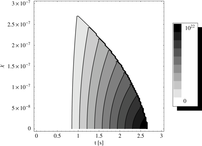
Figure 7: The linearly scaled contour lines of the function $\xi(t,\chi)\,l_{1}$ for $\tilde{\theta}_{\mathrm{max}}=\theta_{\mathrm{max}}$.

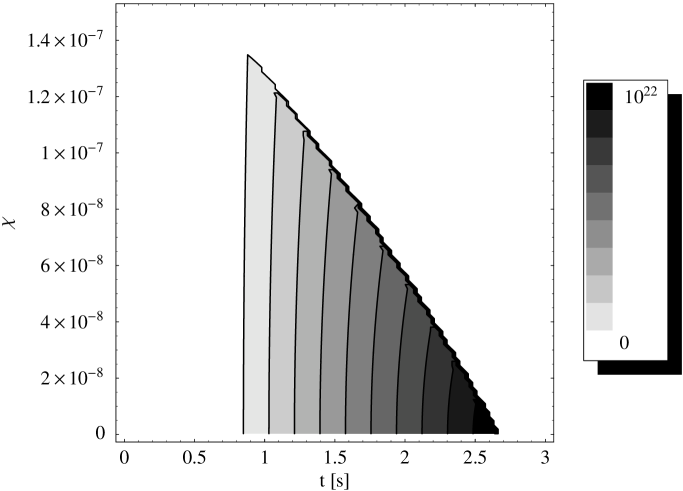
Figure 8: The linearly scaled contour lines of the function $\xi(t,\chi)\,l_{1}$ for $\tilde{\theta}_{\mathrm{max}}=\theta_{\mathrm{max}}/2$.

Note that the $\chi$-scales are different in these two plots. The white regions indicate $\xi=0$, i.e., the integrand in Eq. (60) does not contribute. One can see that the contours of equal $l_{1}$ become quite independent of $\chi$ for small $\tilde{\theta}_{\mathrm{max}}$, i.e., the arrival time $t$ becomes dominated by different velocities due to different masses (cf., Fig. 7). For large $\tilde{\theta}_{\mathrm{max}}$ we can see the effects of the different path lengths, curving the contours towards large $t$, i.e., late arrival, for large $\chi$ (cf., Fig. 8). Thus, in comparison to the example in Sec. 4, we expect enhancements for late time arrivals and suppressions for early time arrivals, because of the delays due to different traveling paths. For the case of Majoron decay in Sec. 5 we demonstrated that for neutrinos the function $\eta(\chi,l_{1})$ is favoring small $\chi$, which means that the approximation $\tilde{\theta}_{\mathrm{max}}\ll\theta_{\mathrm{max}}$ should be good. In this case, the problem reduces to the one in Sec. 4. For antineutrinos, the approximation $\tilde{\theta}_{\mathrm{max}}=\theta_{\mathrm{max}}$ is better.

Figure 9 shows the qualitative behavior of $\Phi^{D,1}_{\alpha e}$ for different $\tilde{\theta}_{\mathrm{max}}$.

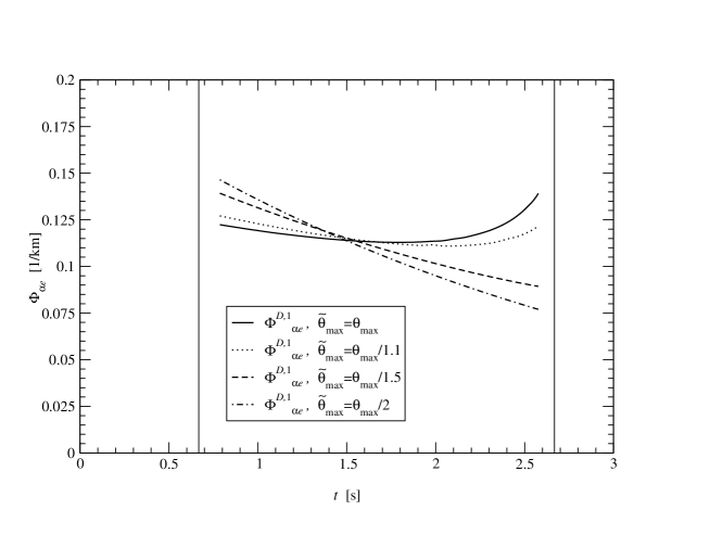
Figure 9: The flux of decay products $\Phi^{D,1}_{\alpha e}$ for the decay rate $\alpha=\alpha_{0}=E/L$ and different values of $\tilde{\theta}_{\mathrm{max}}$.

The vertical lines indicate the arrival times of the light and heavy mass eigenstates on the direct paths, described by the $\delta$-distributions in $\Phi^{D,0}_{\alpha e}$, whereas massless particles would arrive at $t=0$. One can see that the smaller $\tilde{\theta}_{\mathrm{max}}$, the more exponential the time dependence becomes, such as in Sec. 4 for forward traveling only. For large $\tilde{\theta}_{\mathrm{max}}$ late time arrivals are preferred, corresponding to particles delayed by longer path lengths. In principle, some particles could even arrive after the heavy mass eigenstate traveling on the direct path, but these had to decay quite late in order to keep the slow velocity of the heavy mass eigenstate as long as possible. Geometry ($\theta<\theta_{\mathrm{max}}$) implies, however, that we have the shortest overall traveling paths for $l_{1}$ close to $0$ or $L$. This means that this is only possible for the case where path length effects dominate the mass dispersion, i.e., $\tilde{\theta}_{\mathrm{max}}^{ij}\gg\sqrt{\Delta m_{ij}^{2}}/E$, which we do not consider in this example.

In Fig. 10, the effect of different decay rates on $\Phi^{D,1}_{\alpha e}$ is illustrated.

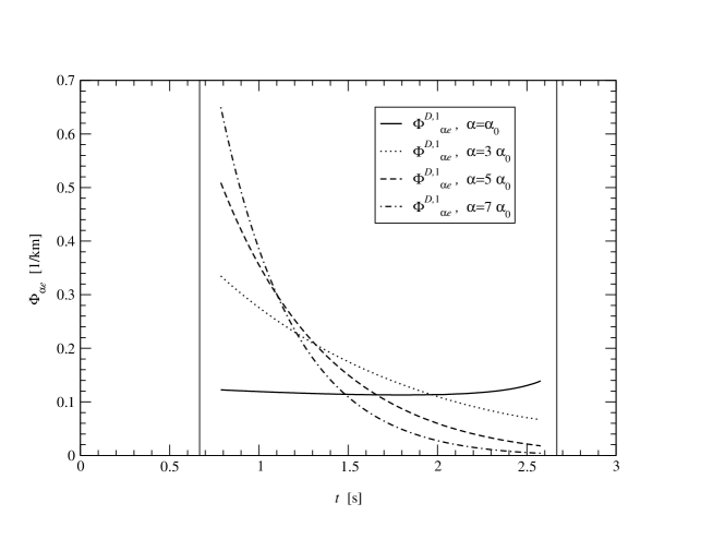
Figure 10: The flux of decay products $\Phi^{D,1}_{\alpha e}$ for $\tilde{\theta}_{\mathrm{max}}=\theta_{\mathrm{max}}$ and different values of decay rates $\alpha$ as multiples of $\alpha_{0}=E/L$.

Note that $\alpha_{0}$ is chosen such that $\alpha_{0}L/E=1$. For larger decay rates we see a behavior closer to the one in Sec. 4, i.e., exponential dropping. In this case, most particles will decay early along the traveling path. Geometry implies in addition that the overall path length is close to its minimum for $l_{1}\simeq 0$. Therefore, for large decay rates path length effects can again be ignored. We conclude that different traveling path lengths only have to be taken into account in computing the supernova neutrino signal for large enough $\tilde{\theta}_{\mathrm{max}}$ and small enough decay rates. However, since $\Phi^{D,1}_{\alpha e}$ is directly proportional to the decay rate, too small decay rates will make the flux $\Phi^{D,1}_{\alpha e}$ vanish.

7 Early coherent decays

As already mentioned above in Sec. 3.3.4, one can see some peculiarities for incoherent propagation over the entire baseline $L$, i.e., $L\gg L^{\mathrm{coh}}$, but for decay before loss of coherence, $\alpha\gg E/L^{\mathrm{coh}}$. Let us again assume a flux pulse $\Phi^{\mathrm{tot}}_{\alpha}=N_{\alpha}\delta(t+L)$. Neglecting corrections to the signal height of the order $m^{2}L/(2E^{2})$, as well as path length dependencies for simplicity, i.e., combing the results of Secs. 3.3.3 and 3.3.4 in a straightforward way, we obtain from Eqs. (34-37)

$${dP_{\alpha\beta}^{1,j}\over dl} = |U_{\beta j}|^{2}\left|\sum\limits_{i}U_{\alpha i}^{*}e^{-\frac{\alpha_{j}(L-l)}{2E}}\sqrt{\alpha_{ij}\over E}e^{-iE_{i}l}e^{-\frac{\alpha_{i}l}{2E}}\right|^{2},$$ (62)

$$\Phi^{D,1}_{\alpha\beta}(t) = \frac{DN_{\alpha}}{4\pi L^{2}}\sum\limits_{j}$$ (63)

$$\times \int\limits_{0}^{L}\delta\left(t+L-l\left(1+{\overline{m^{2}}\over 2E^{2}}\right)-(L-l)\left(1+{m_{j}^{2}\over 2E^{2}}\right)\right){dP_{\alpha\beta}^{1,j}\over dl}dl,$$

where $\overline{m^{2}}$ refers to the mean mass square of the heavy mass eigenstates before decay, as introduced in Sec. 3.3.4. Defining $K_{ijkl}^{\alpha\beta}\equiv U_{\alpha i}^{*}U_{\beta j}U_{\alpha k}U_{\beta l}^{*}$ and assuming the secondary neutrinos are stable, i.e., $\alpha_{j}\equiv 0$, as well as $\Im K=0$, we find after some algebra

$$\Phi^{D,1}_{\alpha\beta}(t) = \frac{DN_{\alpha}}{4\pi L^{2}}\underset{i\neq j,\,k\neq j}{\sum_{i}\sum_{k}\sum_{j}}\frac{2E\sqrt{\alpha_{ij}\alpha_{kj}}}{\overline{m_{ik}^{2}}-m_{j}^{2}}K_{ijkj}^{\alpha\beta}$$

$$\times \exp\left[-\frac{(\alpha_{i}+\alpha_{k})E}{\overline{m_{ik}^{2}}-m_{j}^{2}}\left(t-\frac{m_{j}^{2}}{2E^{2}}L\right)\right]\cos\left[\frac{\Delta m_{ik}^{2}E}{\overline{m_{ik}^{2}}-m_{j}^{2}}\left(t-\frac{m_{j}^{2}}{2E^{2}}L\right)\right].$$

Here $\overline{m_{ik}^{2}}\equiv(m_{i}^{2}+m_{k}^{2})/2$ is evaluated for the heavy mass eigenstates before decay, and the condition $m_{j}^{2}L/(2E^{2})\leq t\ll\overline{m_{ik}^{2}}L/(2E^{2})$, coming from the integration limits, has to be satisfied. This is a very interesting result, since we may see a time-dependent oscillation if two $\alpha_{ij}$’s are non-zero, i.e., if we have two decay channels with only one neutrino decay product. The time $t$ indirectly measures the decay position via the flight time of the decay product. Thus, it also measures the relative phase of the incoming states at this position, which induces the oscillations. However, since all $\alpha$’s are assumed to be quite large, $\alpha\gg E/L^{\mathrm{coh}}$, the exponential indicates that the dominant contribution comes from $t\simeq m_{j}^{2}L/(2E^{2})$. Therefore, only a small fraction of the possible time interval $\Delta t=(\overline{m_{ik}^{2}}-m_{j}^{2})L/(2E^{2})$ will be covered by the signal. The oscillating effect will hence not be observable in most cases. Thus, we have to integrate the observed signal over time, leading to

$$N_{\alpha\beta}^{D,1}\equiv\int\limits_{\frac{Lm_{j}^{2}}{2E^{2}}}^{\frac{\overline{m_{ik}^{2}}L}{2E^{2}}}\Phi_{\alpha\beta}^{D,1}(t)dt=\frac{DN_{\alpha}}{4\pi L^{2}}\underset{i\neq j,\,k\neq j}{\sum_{i}\sum_{k}\sum_{j}}2K_{ijkj}^{\alpha\beta}\frac{\sqrt{\alpha_{ij}\alpha_{kj}}(\alpha_{i}+\alpha_{k})}{(\alpha_{i}+\alpha_{k})^{2}+(\Delta m_{ik}^{2})^{2}}.$$ (65)

In comparison to entirely incoherent propagation without interference of decay channels, which corresponds to $\delta_{ik}$ in the summation, we observe the following two peculiarities:

• Interference of decay channels $\alpha_{ij}\neq 0$, $\alpha_{kj}\neq 0$, and $i\neq k$ creates additional terms in the summation, which, in principle, enhance the number of detectable neutrinos.

• The mentioned interference terms are reduced with increasing $\Delta m_{ik}^{2}$ due to phase shifts in early decays. This reduction can be neglected for $\Delta m_{ik}^{2}\ll\alpha_{i}+\alpha_{k}$, because the decay length is in such a scenario much shorter than the oscillation length and the neutrinos will have decayed before any oscillations. For $\Delta m_{ik}^{2}\gg\alpha_{i}+\alpha_{k}$ the interference terms will vanish by averaging over all possible decay positions and the corresponding phases.

8 Summary and conclusions

In this paper, we have combined neutrino decay and neutrinos oscillations for radially symmetric sources, such as supernovas. We have calculated time-dependent fluxes at the detector by taking into account decoherence due to the long baselines, interference effects within the coherence lengths, time dependence of the source, different flight times of different mass eigenstates, and different traveling paths for neutrinos re-directed in decay. We observed two interesting arrival time dispersion effects, which can in some cases be of the same order of magnitude:

1. The time of arrival depends on the decay position, since for visible neutrino decay products neutrinos travel with different velocities before and after decay. The decay positions are distributed in an exponential manner, which means that we will also observe an exponential decrease of the detected flux in time.

2. The time of flight depends on the path. For radially symmetric sources, neutrinos with different traveling paths arrive at the detector, since decay may change the direction of the secondary neutrinos. This effect suppresses early time arrivals and favors late time arrivals, working in the opposite direction to (1).

We have demonstrated that the first effect can mimic an exponentially decreasing flux at the detector, such that it can be fit to SN1987A data, for very small decay rates. This shows that supernova properties, which are inferred from a description without neutrino decay, can be altered or even completely changed. Moreover, we have shown for Majoron decay that the second effect has only to be taken into account for antineutrinos and not too large decay rates $\alpha L/E\simeq 1$, if the masses of the participating neutrinos are of similar order of magnitude. For the case of $\Delta m_{ij}^{2}\gg m_{j}^{2}$ for active neutrinos, the second effect would be much larger than the one discussed in this paper.

Coherence is not only related to the production process, but also to the detection or decay process. Thus, for small coupling constants in the Lagrangians coherence lengths can in some cases be quite large. In some sense, neutrino decay may act as a “coherence lens” by making the wave packets collapse. However, finite lifetime constraints, such as Eq. (5) for Majoron decay, have to be satisfied in order not to wash out interference effects. There are also some counter-intuitive peculiarities, which may be observed for very large decay rates. Even if only incoherent mass eigenstates (or at least one) arrive at the detector, there may be interference effects modifying the event rates. This is because neutrinos for very early decays may decay as long as they are still coherently propagating. For extreme choices of the masses and decay rates, as well as simultaneous coupling to the decay product by two different mass eigenstates in the Lagrangian (e.g., for Majoron coupling constants $g_{31}\simeq g_{21}\neq 0$), one can, in principle, have a time-dependent oscillation of the signal at the detector. In this case, the sensitivity-dependent neutrino oscillation is transferred into a time dependence of the signal by the time of flight concept of the different mass eigenstates. Note that this may also happen even if only one mass eigenstate is stable, which finally arrives at the detector.

Since extremely small coupling constants in the Lagrangian can cause neutrino decay over typical supernova distances, neutrino decay should always be taken into account in the calculation of transition probabilities and fluxes. The observations of supernova neutrinos from SN1987A indicate so far only that there is at least one stable mass eigenstate. We have shown that a number of effects involving neutrino decay into different mass eigenstates may alter the event rates at the detector even for only one arriving mass eigenstate. Thus, supernova neutrinos are an excellent probe to test neutrino decay. However, similar effects can be induced by details of the supernova explosion, which means that a separation of decay effects and supernova details may be difficult.

References

- [1] J.N. Bahcall, N. Cabibbo and A. Yahil, Phys. Rev. Lett. 28 (1972) 316.
- [2] S. Pakvasa and K. Tennakone, Phys. Rev. Lett. 28 (1972) 1415.
- [3] A. Acker, A. Joshipura and S. Pakvasa, Phys. Lett. B285 (1992) 371.
- [4] V. Barger et al., Phys. Rev. Lett. 82 (1999) 2640, astro-ph/9810121.
- [5] V. Barger et al., Phys. Lett. B462 (1999) 109, hep-ph/9907421.
- [6] G.L. Fogli et al., Phys. Rev. D59 (1999) 117303, hep-ph/9902267.
- [7] P. Lipari and M. Lusignoli, Phys. Rev. D60 (1999) 013003, hep-ph/9901350.
- [8] S. Choubey and S. Goswami, Astropart. Phys. 14 (2000) 67, hep-ph/9904257.
- [9] S. Choubey, S. Goswami and D. Majumdar, Phys. Lett. B484 (2000) 73, hep-ph/0004193.
- [10] A. Bandyopadhyay, S. Choubey and S. Goswami, Phys. Rev. D63 (2001) 113019, hep-ph/0101273.
- [11] R.S. Raghavan, X.G. He and S. Pakvasa, Phys. Rev. D38 (1988) 1317.
- [12] M. Lindner, T. Ohlsson and W. Winter, Nucl. Phys. B607 (2001) 326, hep-ph/0103170.
- [13] G.T. Zatsepin and A.Y. Smirnov, Yad. Fiz. 28 (1978) 1569, Sov. J. Nucl. Phys. 28 (1978) 807.
- [14] Y. Chikashige, R.N. Mohapatra and R.D. Peccei, Phys. Rev. Lett. 45 (1980) 1926.
- [15] G.B. Gelmini and M. Roncadelli, Phys. Lett. B99 (1981) 411.
- [16] S. Pakvasa, hep-ph/0004077.
- [17] J. Schechter and J.W.F. Valle, Phys. Rev. D25 (1982) 774.
- [18] J.A. Frieman, H.E. Haber and K. Freese, Phys. Lett. B200 (1988) 115.
- [19] Y. Aharonov, F.T. Avignone and S. Nussinov, Phys. Lett. B200 (1988) 122.
- [20] J.M. Soares and L. Wolfenstein, Phys. Rev. D40 (1989) 3666.
- [21] A. Acker, S. Pakvasa and R.S. Raghavan, Phys. Lett. B238 (1990) 117.
- [22] C. Giunti, C.W. Kim and U.W. Lee, Phys. Rev. D44 (1991) 3635.
- [23] C. Giunti and C.W. Kim, Phys. Rev. D58 (1998) 017301, hep-ph/9711363.
- [24] W. Grimus, P. Stockinger and S. Mohanty, Phys. Rev. D59 (1999) 013011, hep-ph/9807442.
- [25] T. Ohlsson, Phys. Lett. B502 (2001) 159, hep-ph/0012272.
- [26] C.Y. Cardall, Phys. Rev. D61 (2000) 073006, hep-ph/9909332.
- [27] C.W. Kim and W.P. Lam, Mod. Phys. Lett. A5 (1990) 297.
- [28] G.G. Raffelt, Stars as Laboratories for Fundamental Physics (The University of Chicago Press, Chicago, 1996).
- [29] V. Barger, W.Y. Keung and S. Pakvasa, Phys. Rev. D25 (1982) 907.
- [30] A. Acker, S. Pakvasa and J. Pantaleone, Phys. Rev. D45 (1992) 1.
- [31] M. Kachelrieß, R. Tomàs and J.W.F. Valle, Phys. Rev. D62 (2000) 023004, hep-ph/0001039.
- [32] R. Tomàs, H. Päs and J.W.F. Valle, Phys. Rev. D64 (2001) 095005, hep-ph/0103017.
- [33] J.F. Beacom, Baltimore 1999, Neutrinos in the new millennium, edited by G. Domokos and S. Kovesi-Domokos, p. 357, Singapore, 2000, World Scientific, hep-ph/9909231.
- [34] E. Ma and G. Rajasekaran, Phys. Rev. D64 (2001) 117303, hep-ph/0107203.