Multiple Peaks in the Angular Power Spectrum of the Cosmic Microwave Background: Significance and Consequences for Cosmology

Abstract

Three peaks and two dips have been detected in the power spectrum of the cosmic microwave background from the BOOMERANG experiment, at $\ell\sim 210,540,840$ and $\ell\sim 420,750$, respectively. Using model-independent analyses, we find that all five features are statistically significant and we measure their location and amplitude. These are consistent with the adiabatic inflationary model. We also calculate the mean and variance of the peak and dip locations and amplitudes in a large 7-dimensional parameter space of such models, which gives good agreement with the model-independent estimates, and forecast where the next few peaks and dips should be found if the basic paradigm is correct. We test the robustness of our results by comparing Bayesian marginalization techniques on this space with likelihood maximization techniques applied to a second 7-dimensional cosmological parameter space, using an independent computational pipeline, and find excellent agreement: $\Omega_{\rm tot}=1.02^{+0.06}_{-0.05}$ vs. $1.04\pm 0.05$, $\Omega_{b}h^{2}=0.022^{+0.004}_{-0.003}$ vs. $0.019^{+0.005}_{-0.004}$, and $n_{s}=0.96^{+0.10}_{-0.09}$ vs. $0.90\pm 0.08$. The deviation in primordial spectral index $n_{s}$ is a consequence of the strong correlation with the optical depth.

1 Introduction

BOOMERANG has recently produced an improved power spectrum ${\cal C}_{\ell}$ of the cosmic microwave background (CMB) temperature anisotropy ranging from $\ell\sim 100$ to $\ell\sim 1000$ (Netterfield et al., 2001, hereafter B01). Three peaks are evident in the data, the first, at $\ell\sim 210$ confirms the results of previous analysis of a small subset of the BOOMERANG data set (de Bernardis et al, 2000, hereafter B00) as well as results from other experiments (see e.g. Miller et al., 1999; Mauskopf et al., 2000; Hanany et al., 2000). Analysis of the bulk of the remaining data has improved the precision of the power spectrum and extended the coverage to $\ell\sim 1000$, revealing for the first time a second peak at $\ell\sim 540$, and a third at $\ell\sim 840$.

The results of two other experiments, released simultaneously with B01, are in good agreement with the BOOMERANG data. In addition to the first peak, the results from DASI (Halverson et al., 2001) show a peak coincident with that seen in our data near $\ell\sim 540$, and a rise in the spectrum toward high $\ell$ that is consistent with the leading edge of the peak seen in our data near $\ell\sim 840$. The results from MAXIMA (Lee et al., 2001) are of lower precision, but are consistent with both the DASI and the BOOMERANG results.

These detections are the first unambiguous confirmation of the presence of acoustic oscillations in the primeval plasma before recombination (Peebles et al., 1970; Sunyaev & Zeldovich, 1970), as expected in the standard inflationary scenario (Bond & Efstathiou, 1987).

If the adiabatic cold dark matter (CDM) model with power-law initial perturbations describes our cosmogony, then the angular power spectrum of the CMB temperature anisotropy is a powerful tool to constrain cosmological parameters (see e.g. Kamionkowski & Kosowsky, 1999, and references therein).

In B01 a rigorous parameter extraction has been carried out with the methods of Lange et al. (2001), significantly improving the constraints obtained from previous CMB analyses (see e.g. Dodelson & Knox, 2000; Melchiorri et al., 1999; Lange et al., 2001; Balbi et al., 2000; Tegmark & Zaldarriaga, 2000; Jaffe et al., 2001; Kinney et al., 2000; Bond et al., 2000; Bridle et al., 2000) on key cosmological parameters.

Furthermore, the new BOOMERANG spectrum gives a value for the baryon fraction $\Omega_{b}h^{2}$ that is in excellent agreement with independent constraints from standard big bang nucleosynthesis (BBN), eliminating any hint of a conflict between the BBN and the CMB-derived values for the baryon density (see e.g. Peebles et al., 2000).

In this paper we support the conclusions of B01 by presenting two complementary analyses of the measured power spectrum. In Section 2 we briefly compare these latest BOOMERANG results with those of B00. In Section 3, using “model-independent” methods similar to that used in Knox & Page (2000), we measure the positions and amplitudes of the peaks in the spectrum. We also compute the probability distribution of the theoretical power spectra used in B01 given the measured $C_{\ell}$’s to estimate the averages and variances of the peaks and dips, as in Bond et al. (2000).

In Section 4, we extract the distribution of cosmological parameters using a different grid of theoretical power spectra and a different method for projecting onto one and two variable likelihoods than that used in B01, and show good agreement between the two methods. The B01 ${\cal C}_{\ell}$-database used the cosmological parameter set $\{\Omega_{tot}$, $\Omega_{\Lambda}$, $\Omega_{b}h^{2}$, $\Omega_{c}h^{2}$, $n_{s}$, $\tau_{C}$, ${\cal C}_{10}\}$, where $n_{s}$ is the spectral index of primordial density fluctuations, $\Omega_{c}$ and $\Omega_{\Lambda}$ are the cold dark matter and vacuum energy densities in units of the critical density, and ${\cal C}_{10}$ is an overall normalization of the power spectrum. The alternate grid described here uses $\Omega_{b}$, $\Omega_{m}\equiv\Omega_{c}+\Omega_{b}$ and the Hubble parameter $h$ instead of $\Omega_{b}h^{2}$, $\Omega_{c}h^{2}$ and $\Omega_{tot}=\Omega_{m}+\Omega_{\Lambda}$, which are now derived parameters.

The determination of cosmological parameters is affected by the presence of near-degeneracies among them (Efstathiou & Bond, 1999). In B01 and Lange et al. (2001), this is improved through the use of parameter combinations which minimize the effects of these degeneracies, except for the important one between $\Omega_{tot}$ and $\Omega_{\Lambda}$. However, as long as the database is sufficiently extensive and finely gridded, one should get nearly the same answer. In addition to using different parameter choices to generate one and two dimensional likelihood functions, we use likelihood maximization rather than marginalization (integration) over the other variables. Maximization could have a different (and often more conservative) response to the presence of degeneracies in the model space. We obtain excellent agreement between the two treatments, and also show that when we apply our methods to the DASI data, we get the same results as Pryke et al. (2001). In Section 5 we report our conclusions.

2 The Power Spectrum: Comparison with Previous Results

The first results from the 1998/99 flight of BOOMERANG were reported one year ago by B00. These included the first resolved images of the CMB over several percent of the sky, and a preliminary power spectrum based on analysis of a small fraction of the data. The power spectrum obtained by B01 incorporates a 14-fold increase in effective integration time, and an $\sim 1.8$-fold increase in sky coverage. Thus, the B01 result obtains higher precision both at low $\ell$, where the precision is limited by sample variance, and at high $\ell$, where it is limited by detector noise. Moreover, the B01 results make use of an improved pointing solution that has led to qualitative improvements in our knowledge of the physical beam and our understanding of the pointing jitter, which adds in quadrature with the physical beam to give the effective angular resolution of the measurement.

We now understand that the pointing solution used in B00 produced an effective beam size of $(12.7\pm 2.0)$ arcmin, rather than the $(10\pm 1)$arcmin assumed in that analysis, due to an underestimate of the pointing jitter. The effect of underestimating the effective beamwidth is to suppress the power spectrum at small angular scales. However, this is not the reason preventing the detection of a second peak from that dataset. In fact, when the effects of the pointing jitter are corrected for, the signal-to-noise ratio of the B00 spectrum at $\ell>350$ is still insufficient to detect the second peak, and the data are still compatible with flat bandpower. In Fig. 1 we plot the spectrum of B00 corrected for the jitter underestimate and for an overall gain adjustment ($+20\%$ in ${\cal C}_{\ell}$, within the $\pm 20\%$ uncertainty assigned to the absolute calibration in both B00 and B01). The corrected B00 spectrum is in excellent agreement with the B01 spectrum.

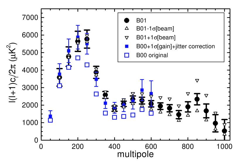
Figure 1: The angular power spectrum of the CMB measured by BOOMERANG. The filled circles are the spectrum reported by B01; the up and down triangles indicate the systematic error in B01 resulting from the error in the beam. Three peaks are visible at multipoles $\sim 210,\sim 540,\sim 840$. The open squares are the spectrum reported by B00, based on an analysis of $\sim 7\%$ of the data analyzed in B01. The filled squares present the B00 spectrum after correction for pointing jitter and scaled by 10$\%$ ($1\sigma$) in overall calibration (see text).

The data of B00 have been used to derive $\Omega_{tot}$ in the same paper, and to derive a full set of cosmological parameters in Lange et al. (2001). The cosmological result of B00 - that the geometry of the universe is nearly flat - is not altered by the correction, since the correction does not move significantly the location of the first peak. That analysis was done assuming a ”medium” prior on $h$ and $\Omega_{b}h^{2}$. When the full parameter analysis is done, assuming weaker priors as in Lange et al. (2001), the effect of the correction is to drive $\Omega_{tot}$ even closer to unity. With the new data set of B01, $\Omega_{tot}=1.04^{+0.08}_{-0.07}$ using the $\ell<600$ part of the new data, $\Omega_{tot}=1.02^{+0.06}_{-0.05}$ with all of it.

The largest effect of the correction is on the baryon density derived in Lange et al. (2001). The uncorrected spectrum gives a baryon density $\Omega_{b}h^{2}=0.036^{+0.006}_{-0.005}$ for the ”weak” prior case. The value derived from the B01 spectrum if only the data at $\ell\leq 600$ are used is $0.027^{+0.005}_{-0.005}$. Adding the data at higher $\ell$ removes degeneracies and further reduces the value to $0.022^{+0.004}_{-0.003}$, as described below.

3 Significance and Location of the Peaks and Dips

In this section we investigate the significance of the detection of peaks and dips in our data, and estimate their locations using both model-independent, frequentist methods and model-dependent, Bayesian methods.

Table 1: Peaks and dips: location and amplitude.

		$\ell_{\rm p}$			${\cal C}_{\rm p}$ ($\mu K^{2}$)
Features	model independent	no priors	weak	model independent	no priors	weak
Peak 1	$213^{+10}_{-13}$	$220\pm 7$	$221\pm 5$	$5450^{+1200}_{-1100}$	$5440^{+1300}_{-1050}$	$5140^{+1280}_{-1030}$
Dip 1	$416^{+22}_{-12}$	$413\pm 12$	$412\pm 7$	$1850^{+440}_{-410}$	$1640^{+390}_{-320}$	$1590^{+390}_{-320}$
Peak 2	$541^{+20}_{-32}$	$539\pm 14$	$539\pm 8$	$2220^{+560}_{-520}$	$2480^{+620}_{-500}$	$2420^{+630}_{-500}$
Dip 2	$750^{+20}_{-750}$	$688\pm 22$	$683\pm 23$	$1550^{+550}_{-610}$	$1530^{+470}_{-360}$	$1590^{+500}_{-380}$
Peak 3	$845^{+12}_{-25}$	$825\pm 21$	$822\pm 21$	$2090^{+790}_{-850}$	$2170^{+720}_{-540}$	$2270^{+760}_{-570}$
Dip 3	-	$1025\pm 24$	$1024\pm 26$	-	$880^{+290}_{-220}$	$910^{+310}_{-230}$
Peak 4	-	$1139\pm 24$	$1138\pm 24$	-	$1100^{+380}_{-280}$	$1130^{+400}_{-290}$
Dip 4	-	$1328\pm 31$	$1324\pm 33$	-	$570^{+220}_{-160}$	$610^{+240}_{-170}$
Peak 5	-	$1442\pm 30$	$1439\pm 32$	-	$680^{+290}_{-200}$	$730^{+310}_{-220}$
Dip 5	-	$1661\pm 37$	$1660\pm 36$	-	$300^{+130}_{-90}$	$320^{+130}_{-90}$

Note. — Location (columns 2-4) and amplitude (columns 5-7) of peaks and dips in the power spectrum of the CMB measured by BOOMERANG. In column 2 we list the values measured by means of a parabolic fit to the bandpowers ($\Delta\ell=50$). In columns 3 and 4 we list the values estimated by integrating the peak and dip properties of the theoretical spectra used in Lange et al. (2001) and B01 over the probability distribution for the database, assuming either the no prior or weak prior restrictions of those papers. In column 5,6,7 we do the same for the amplitude of the peaks. Note that Peaks 4 and 5, and Dips 3, 4, 5 are all outside the range directly measured, so they are forecasts of what is likely to emerge if the database has components that continue to describe the data well, as they do now. All the errors are at 1-$\sigma$ and include the effect of gain and beam calibration uncertainties. 2-$\sigma$ confidence intervals can be significantly broader than twice the 1-$\sigma$ intervals reported here, as is clear from Fig. 2.

3.1 Model-Independent Analyses of Peaks and Dips

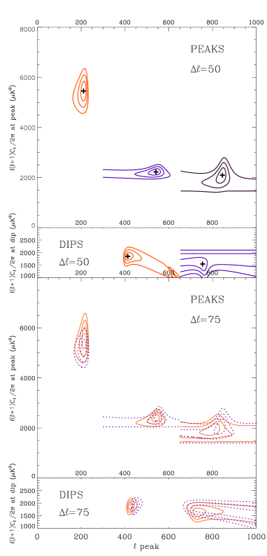
Figure 2: $\Delta\chi^{2}$ contours for the position and amplitude of the peaks and dips in the BOOMERANG CMB temperature power spectrum. The crosses in the two upper panels correspond to the minima for the $\chi^{2}$; the three contours are plotted at $\Delta\chi^{2}=2.3,6.17,11.8$ (corresponding to 68.3$\%$, 95.4$\%$, 99.7$\%$ confidence intervals for a gaussian likelihood in two parameters). The two upper panels refer to a $\Delta\ell=50$ binning of the power spectrum. The multipole ranges used for the parabolic fits on peak 1, dip 1, peak 2, dip 2 and peak 3 are (76 - 375), (276 - 475), (401 - 750), (676 - 875) and (726 -1025) respectively. The two lower panels refer to binnings with $\Delta\ell=75$. While the statistical significance of the detections is improved, the location of the features is less robust against the centering of the bins: continuous and dashed lines refer to bin centers shifted by 35.

3.1.1 Does a Flat Spectrum Fit the Data?

As a first step, we answer the question, ”How likely is it that the measured bandpowers ${\cal C}_{\ell}$ are just fit by a first order polynomial ${\cal C}_{\ell}^{T}={\cal C}_{A}+{\cal C}_{B}\ell$”. Since the first peak is evident, we limit this analysis to the data bins centered at $450\lower 2.15277pt\hbox{$\;\buildrel<\over{\sim}\;$}\ell\lower 2.15277pt\hbox{$\;\buildrel<\over{\sim}\;$}1000$. We compute $\chi^{2}=({\cal C}_{b}-{\cal C}_{b}^{T})M^{-1}_{bb^{\prime}}({\cal C}_{b^{\prime}}-{\cal C}_{b^{\prime}}^{T})$, where $M_{bb^{\prime}}$ is the covariance matrix of the measured bandpowers ${\cal C}_{b}$ and ${\cal C}_{b}^{T}$ is an appropriate band average of ${\cal C}_{\ell}$. For this exercise, we used a Gaussian distribution in the ${\cal C}_{b}^{T}$, but have also checked a lognormal in ${\cal C}_{b}^{T}$, with $M$ suitably transformed. We find similar answers using these two limits of the offset-lognormal distribution for the bandpowers recommended by Bond, Jaffe & Knox (2000). We vary ${\cal C}_{A}$ and ${\cal C}_{B}$ to find the minimum of the $\chi^{2}$, $\chi^{2}_{\rm min}$, and compute the probability of having a $\chi^{2}<\chi^{2}_{\rm min}$. A first order polynomial is rejected in all cases. $P(\chi^{2}<\chi^{2}_{\rm min})$ is 95.2$\%$, 96.5$\%$, 94.8$\%$ for the multipole ranges 401-1000, 401-750, 726-1025 respectively (using a binning of $\Delta\ell=75$ for the bandpowers). These conclusions are robust with respect to variations in the location and width of the $\ell$-ranges, as well as for variations of the beam FWHM allowed by the measurement error. We conclude that the features measured in the spectrum are statistically significant at approximately $2\sigma$.

3.1.2 Peak and Dip Location and Amplitude Likelihood Maps

We now describe some methods we have used to locate the peaks and dips of the power spectrum. Results shown in Table 1 used a parabolic fit for ${\cal C}_{\ell}$. (As described below, we have also used parabolas in $\ln{\cal C}_{\ell}$. The use of more complex functions, see e.g. Knox & Page (2000), is not required by the data.) The criterion for robust peak/dip detection is that the mean curvature of the parabola be above some threshold (e.g., some multiple of the rms deviation in the curvature). For the model-independent entries of Table 1, for each amplitude ${\cal C}_{\rm p}$ and location of the peak $\ell_{\rm p}$, we found the curvature which gave minimum $\chi^{2}({\cal C}_{\rm p},\ell_{\rm p})$. We repeat this procedure for different data ranges. The contours corresponding to $\Delta\chi^{2}$ of ($2.3$,$6.17$ and $11.8$) are plotted in Fig. 2 for the ranges where this procedure provides a detection of both ${\cal C}_{\rm p}$ and $\ell_{\rm p}$. Three peaks and two dips are clearly detected by this procedure, at the multipoles and with the amplitudes reported in the table. The curvature is required to be negative for peak detection, positive for dip detection. Note that zero curvature is equivalent to the flat bandpower case. Approaching this zero curvature limit is why the contours sometimes open up in $\ell_{\rm p}$ at $\sim 2\sigma$ and become horizontal at $\sim 3\sigma$. This is a visual reiteration of the point made above, that the flat ${\cal C}_{\ell}$ is rejected at about 2$\sigma$. We have found that the location of the peaks is robust against variations of the gain and beam calibration inside the reported error intervals, $10\%$ for the gain calibration error, producing a $20\%$ error in the ${\cal C}_{\rm p}$, and $1.4^{\prime}(1\sigma)$ corresponding to $13\%$ in the beam. The different best fit parabolas for the peaks and dips of the BOOMERANG power spectrum are shown in Fig. 3.

3.1.3 Fisher Matrix Approach with Sliding Bands

We have tried a number of other model-independent peak/dip finding algorithms on the data. For the parabolic model in $\ell$ for $\ln{\cal C}_{\ell}$, we analyzed the quadratic form in blocks of 3, 4 or 5 bins, each bin being of width $\Delta\ell=50$, determining the best fit and the variance about it as defined by the inverse of the likelihood curvature matrix (Fisher matrix). For this exercise, we adopted a lognormal distribution of the bandpowers (but checked for robustness by also assuming a Gaussian distribution) and marginalized over the beam uncertainty. We slid across the $\ell$-space with our fixed bin group and estimated the significance of the peak or dip detection by the ratio of the best-fit curvature to the rms deviation in it. For BOOMERANG, using three bins of width $\Delta\ell=50$ gives stronger detection, but results in larger error bars (as estimated from the inverse Fisher matrix). Here, we quote our 5-bin results, and among these we use for each peak/dip the 5-bin template which gives the largest ratio of the mean curvature to standard deviation of the curvature.

We find interleaved peaks and dips at $\ell=$ $215\pm 11$, $431\pm 10$, $522\pm 27$, $736\pm 21$ and $837\pm 15$. The error bars quoted correspond to the variance in peak position $\ell_{\rm p}$ given the curvature of the parabola fixed at the best-fit value ( if one attempts to marginalize over the curvature, $\ell_{\rm p}$ loses localization due to contribution from fits with vanishing curvature, i.e. straight lines). The amplitudes of the features are $5760^{+344}_{-324}$, $1890^{+196}_{-178}$, $2290^{+330}_{-290}$, $1640^{+500}_{-380}$ and $2210^{+900}_{-640}$ $\mu K^{2}$, correspondingly. When the 10% calibration uncertainty is included, the errors are similar to those in Table 1, but of course the estimates move up and down together in a coherent way, so here we have chosen to indicate the purely statistical error bars. The significance of the detection as estimated by the distinction of the best-fit curvature from zero is $1.7\,\sigma$ for the second peak and dip, and $2.2\,\sigma$ for the third peak.

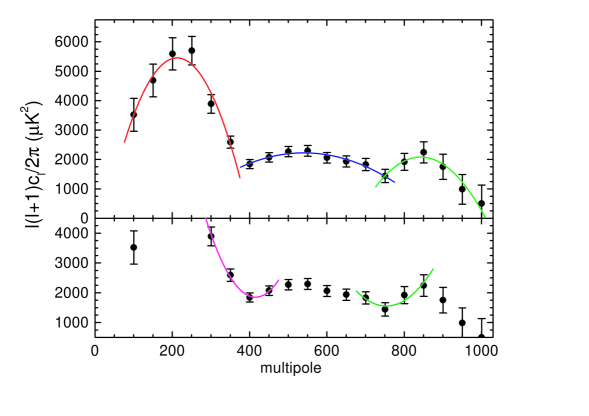
Figure 3: Best fit parabolas for the different peaks and dips of the BOOMERANG spectrum.

3.2 Model-Dependent Analysis of Peaks and Dips

3.2.1 Ensemble-Averaging Method

We have also estimated peak/dip positions and amplitudes on a large set of prescribed ${\cal C}_{\ell}$ shapes weighted by the probability that each shape has when confronted with the data. For the cases shown in Table 1, the prescribed shapes are the elements of the ${\cal C}_{\ell}$ database used in Lange et al. (2001) and B01. Explicitly, we compute for the BOOMERANG+DMR data the ensemble averages $<\ln\ell_{\rm p}>$ and $<\ln C_{\rm p}>$ and their variances, $<(\Delta\ln\ell_{\rm p})^{2}>$, and $<(\Delta\ln C_{\rm p})^{2}>$, with respect to the product of the likelihood function for the parameters and their prior probability. Two cases are shown, for the no prior and weak prior cases of Lange et al. (2001). Note the good agreement using this method with the model-independent results. (The results are nearly the same if we use $<\ell_{\rm p}>$ instead of $<\ln\ell_{\rm p}>$.) When this method was applied to all of the CMB data published before 2001, including that of BOOMERANG and Maxima, a first peak location of $212\pm 7$ was obtained (Bond et al., 2000).

3.2.2 Forecasting Peaks and Dips

One virtue of this procedure is that, because we know the spectral shape for all $\ell$, we can forecast where peaks and dips will lie beyond the $\ell$-region we observe. Thus, Table 1 gives predictions for the locations and amplitudes of the subsequent (4,5) peaks and (3,4,5) dips.

To test whether this works using just the data at hand, we restrict ourselves to using only the $\ell<600$ data and see how well the peaks beyond are found. As expected, the features with $\ell<600$ are quite compatible with those in Table 1 derived using all of the data: for the weak prior case, the first peak, the first dip and the second peak for $\ell<600$ are found to be at $\ell=$ $219\pm 5$, $403\pm 10$ and $530\pm 23$, with amplitudes $6000^{+1450}_{-1160}$, $1750^{+440}_{-350}$ and $2700^{+750}_{-590}$ $\mu K^{2}$. The second dip and third peak are out of range, predicted to be found at $\ell=$ $640\pm 49$ and $789\pm 40$, with amplitudes $2080^{+790}_{-570}$ and $3160^{+1410}_{-980}$ $\mu K^{2}$, in good agreement with the $\ell=$ $683\pm 23$ and $822\pm 21$, with amplitudes $1590^{+500}_{-380}$ and $2270^{+760}_{-570}$ $\mu K^{2}$ actually found. If we further restrict the prior probabilities, the forecasted positions can move a bit: e.g., we find the $\ell<600$ cut with the weak prior gives $\Omega_{tot}=1.04\pm 0.07$, suggesting a constraint to the theoretically-motivated flat universe is reasonable. If we adopt as well the “large scale structure” prior of Lange et al. (2001), we get $\ell=$ $653\pm 45$ and $798\pm 41$ at amplitudes $1950^{+580}_{-450}$ and $2900^{+990}_{-740}$ $\mu K^{2}$; and the fourth peak for $\ell<600$ is forecasted to be at $\ell=1107\pm 46$, similar to the $\ell=1138\pm 24$ forecast of the table. Our conclusion is that even if we restrict ourselves to $\ell<600$, the forecasts are very good. We expect that using all of the data to $\ell=1000$, with multiple peaks and dips, the forecasts of the Table should be even more accurate.

3.3 Peak and Dip Finding in the DASI data

We have applied the sliding band procedure of Section 3.1.3 to the DASI data using the 3-band and 4-band sliders. For the 3-band, we find the first two peaks and interleaving dip at $\ell=$ $202\pm 15$, $407\pm 14$ and $548\pm 10$, with amplitudes $5200^{+530}_{-480}$, $1590^{+163}_{-148}$ and $2760^{+270}_{-250}$ $\mu K^{2}$. Again, we have not included the coherent 8% calibration uncertainty (16% in ${\cal C}_{\ell}$) in these ${\cal C}_{\rm p}$ numbers. It may seems quite incongruous that the error bars on the peak and dip positions can be so small relative to the bin size, but we emphasize that these give the error contours in the immediate neighborhood of the maximum, as described by the Fisher matrix. Just as in Fig. 2, the contours open up at levels lower than 1$\sigma$, resulting in imprecise localization at the 2$\sigma$ level. DASI’s detection of the second dip is 1.6$\sigma$ in curvature by the Fisher error accounting, but it is found, at $\ell=$ $656\pm 19$ and ${\cal C}_{\rm d}=1650^{+260}_{-220}\mu K^{2}$.

We have also applied the prescribed shape method of Section 3.2.1 to the DASI data (Halverson et al., 2001). We find that the location and forecasts are quite compatible with those given in Table 1 for BOOMERANG. For example, for the weak prior, the first three peaks and interleaved two dips are at $\ell=$ $216\pm 6$, $401\pm 10$, $523\pm 12$, $655\pm 30$ and $794\pm 30$, with amplitudes $5240^{+1310}_{-1050}$, $1570^{+370}_{-300}$, $2410^{+590}_{-470}$, $1690^{+410}_{-330}$ and $2480^{+660}_{-520}$ $\mu K^{2}$. These ${\cal C}_{p}$ now include the $8\%$ calibration uncertainty. The forecasted third dip is at $\ell=988\pm 34$ with amplitude $980^{+260}_{-200}\mu K^{2}$, compatible with the BOOMERANG result.

4 Robustness of Cosmological Parameters

The multiple peaks and dips are a strong prediction of the simplest class of adiabatic inflationary models, and more generally of models with passive, coherent perturbations (e.g. Albrecht et al., 1996). Although the main effect giving rise to them is regular sound compression and rarefaction of the photon-baryon plasma at photon decoupling, there are a number of influences that make the regularity only roughly true. Nonetheless, the “catalogue” of peak and dip positions used to construct the table could be searched to find best-fitting sequences and the associated cosmological parameters giving rise to them. Indeed we know that peaks and dips and only a few points in between are enough to characterize the morphology of the ${\cal C}_{\ell}$ spectra (e.g. Sigurdson & Scott, 2000). However, it is clear that it is better to work with the full shapes to test the theories. In this section, we show that the extracted cosmological parameters using the full shapes are robustly determined, by comparing results for the ${\cal C}_{\ell}$ database and Bayesian marginalization techniques used in Lange et al. (2001) and B01 with those obtained using the variables and likelihood maximization techniques described below and in de Bernardis et al. (1997), Dodelson & Knox (2000), Melchiorri et al. (1999) and Balbi et al. (2000). We also test our methods on the DASI data set.

4.1 Extraction of Cosmological Parameters

The $\{\Omega_{m},\Omega_{b},\Omega_{\Lambda},h,n_{s},\tau_{C},C_{10}\}$ space has parameters sampled as follows: $\Omega_{m}=0.11,...,1.085$, in steps of 0.025; $\Omega_{b}=0.015,...,0.20$, in steps of 0.015; $\Omega_{\Lambda}=0.0,...,0.975$, in steps of 0.025; $h=0.25,...,0.95$, in steps of 0.05; spectral index of the primordial density perturbations $n_{s}=0.50,...,1.50$, in steps of 0.02, $\tau_{C}=0.,..,0.5$, in steps of 0.1. The overall amplitude ${\cal C}_{10}$, expressed in units of ${\cal C}_{10}^{COBE}$, is allowed to vary continuously. The theoretical models are computed using the cmbfast program (Seljak & Zaldarriaga, 1996), as were those used in B01. Here, we have ignored the role gravity waves may play. We used the new BOOMERANG anisotropy power spectrum expressed as $18$ bandpowers from $\ell=70$ to $\ell=1050$ (see B01) and we computed the likelihood for the cosmological models as $\exp(-\chi^{2}/2)$, where $\chi^{2}$ is the quadratic form defined in section 3.1.1. A $10\%$ Gaussian-distributed calibration error in the gain and a 1.4’ (13%) beam uncertainty were included in the analysis. The COBE-DMR bandpowers used were those of Bond, Jaffe, and Knox (1998), obtained from the RADPACK distribution (Knox, 2000). For the other ${\cal C}_{\ell}$ database in which $\Omega_{k}=1-\Omega_{tot}$ replaces $\Omega_{m}$ and $\Omega_{c}h^{2}$ and $\Omega_{b}h^{2}$ replace $h$ and $\Omega_{b}$, the parameter grid, the treatment of beam and calibration uncertainty, the use of the offset-lognormal approximation, and the marginalization method, are as described in Lange et al. (2001).

As discussed in Lange et al. (2001), apart from the inevitable database discreteness, assuming a uniform distribution in the variables of the database is tantamount to adopting different relative prior probabilities on the variables. Of course, this is not an issue for the maximization method, and even for marginalization is a very weak prior relative to the strong observed detections. We can use further “top hat” priors to mimic the $\{\Omega_{m},\Omega_{b},h\}$ database by restricting the wide coverage we have in the $\{\Omega_{k},\Omega_{b}h^{2},\Omega_{c}h^{2}\}$ variables. We illustrate this in Fig. 4, where this mimicking prior is coupled to a weak cosmological prior, requiring the age of the Universe to be above 10 Gyr and the Hubble parameter to be in the range 0.45 to 0.85. This is very similar to the weak prior of Lange et al. (2001), Jaffe et al. (2001) and B01, except the upper limit was 0.95: this results in only tiny differences in the extracted parameters.

4.2 Cosmological Parameter Results

Our basic results, on method testing and cosmological implications, are shown in Fig. 4 and the associated contour plots Figs. 5 and 6. Fig. 4 clearly shows that it does not make that much difference in constructing the likelihood function for a target cosmological variable if we marginalize (integrate) over the other cosmological parameters or find the maximum likelihood value. Nor does it matter which database is used. Similar success in agreement is found with other prior choices, but for this paper we will restrict ourselves to the $0.45<h<0.85$ weak prior. When we integrate the distributions of Fig. 4 to get the 50% value and the 1-sigma errors derived from the 16% and 84% values, we obtain $\Omega_{tot}=1.02^{+0.06}_{-0.05}$, $1.02^{+0.05}_{-0.06}$, $1.04\pm 0.05$, for marginalization and maximization in the Lange et al. (2001) ${\cal C}_{\ell}$-database and the maximization in the alternate database, respectively; we also obtain $n_{s}=0.96^{+0.10}_{-0.09}$, $0.90^{+0.09}_{-0.09}$, $0.90\pm 0.06$, and $\Omega_{b}h^{2}=0.022^{+0.004}_{-0.003}$, $0.020^{+0.004}_{-0.004}$, $0.019^{+0.005}_{-0.004}$.

We have also applied the B01 ${\cal C}_{\ell}$ database with marginalization to the DASI data, and find for our $0.45<h<0.95$, age $>10$ Gyr, prior $\Omega_{tot}=1.05^{+0.06}_{-0.06}$, $n_{s}=1.02^{+0.10}_{-0.09}$ and $\Omega_{b}h^{2}=0.024^{+0.005}_{-0.004}$, to be compared with the Pryke et al. (2001) values of $1.05^{+0.06}_{-0.06}$, $1.01^{+0.09}_{-0.07}$ and $0.022^{+0.004}_{-0.004}$. As mentioned above, the overlap of 20% of the DASI fields one the sky precludes a rigorous joint analysis of the datasets. If you proceed anyway as an exercise and ignore those correlations, the results are very close to the BOOMERANG+DMR marginalization values given above, with very slightly reduced errors.

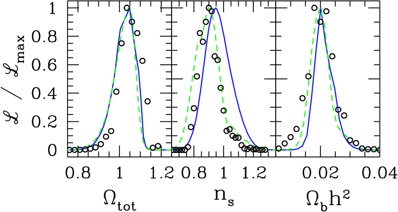
Figure 4: Likelihood curves derived from the BOOMERANG and COBE/DMR datasets as a function of $\Omega_{tot}$, $n_{s}$ and $\Omega_{b}h^{2}$ show the relative insensitivity to whether marginalization over the other variables is done (solid) or the maximum likelihood point in the other variables is chosen (dashed). These curves were constructed using a prior on the ${\cal C}_{\ell}$-database used in B01 designed to mimic the ranges in the alternate ${\cal C}_{\ell}$-database that uses $\{\Omega_{b},\Omega_{m},h\}$ (open circles). A further weak prior, with $0.45<h<0.85$ and age $>10$ Gyr, was used. The high degree of correlation of $n_{s}$ with $\tau_{C}$ accounts for the wider distribution of the marginalized $n_{s}$ likelihood compared to that for the maximization procedure.

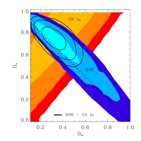
Figure 5: Constraints in the $\Omega_{m}$ vs. $\Omega_{\Lambda}$ plane from the combined BOOMERANG and COBE/DMR datasets, assuming the weak prior $0.45<h<0.85$, age $>10$ Gyr. For this plot, the likelihood at each point is calculated by maximizing over the remaining $5$ parameters. The shaded regions correspond to the $68.3\%$, $95.4\%$ and $99.7\%$ confidence levels. The CMB contours (labeled B98) are overlaid on the contours derived from observations of high redshift supernovae (labeled SN 1a). The line contours are for the combined likelihood.

We now discuss the implications of these determinations in more detail. If we knew all other variables, the position of the first peak would allow us to determine the mean curvature of the universe, and all subsequent dips and peaks would have to follow in a specific set pattern. However, degeneracies among cosmological parameters are present. In particular, there is a geometrical degeneracy between $\Omega_{\Lambda}$ and $\Omega_{tot}$ in the angular diameter distance, which allows the peak/dip pattern to be reproduced by different combinations of the two. The peak/dip heights also have near-degeneracies associated with them, but these can be strongly broken as more peaks and dips are added. Extreme examples are closed models dominated by baryonic dark matter, which can reproduce the observed position of the first peak (Griffiths et al., 2001) but are unable to account for the observed $\ell>600$ power.

The classic $\Omega_{m}$ vs. $\Omega_{\Lambda}$ plot in Fig. 5 shows $68.3\%$, $95.4\%$ and $99.7\%$ contours, defined to be where the likelihood falls to $0.32$, $0.05$ and $0.01$ of its peak value, as it would be for a 2D multivariate Gaussian. The phase space of models in the $\Omega_{m}$ vs. $\Omega_{\Lambda}$ plane results in the likelihood for the total energy density of the universe $\Omega_{\rm tot}$ being skewed towards closed models (see e.g. Lange et al., 2001; Bond et al., 2000). This skewness is not important if the acceptable model space is well localized, which can be accomplished by imposing prior probabilities, in particular on $h$. The weak “top hat $h=0.65\pm 0.20$” prior we have adopted decreases the skewness to closed models (which is quite evident if models with very low $h$ values are included, as described in B01, and helps to break the geometrical degeneracy, hinting at the presence of a cosmological constant at the level of $\sim 1\sigma$. This becomes more pronounced with a stronger prior on $h$ (B01). Including the recent supernovae data Perlmutter et al. (1997) with the weak prior used here, we find $\Omega_{\Lambda}=0.71\pm 0.11$ and $\Omega_{m}=0.31^{+0.13}_{-0.12}$ using maximization, to be contrasted with the marginalization results using the B01 database of $0.73^{+0.07}_{-0.10}$ and $0.32\pm 0.06$.

The measurement of the relative amplitude of the peaks in the CMB spectrum provides important constraints on the physical density of baryons $\Omega_{b}h^{2}$. In the region from $\ell\sim 50$ and up to the second peak, $\Omega_{b}h^{2}$ is nearly degenerate with variations in the primordial spectral index of scalar fluctuations $n_{s}$: increasing $\Omega_{b}h^{2}$ increases the ratio of the amplitudes of the first and second peaks, but so does decreasing $n_{s}$. Beyond the second peak, however, the two effects separate: the third peak rises by increasing $\Omega_{b}h^{2}$ and lowers by decreasing $n_{s}$. Thus, though Fig. 6 shows that the two are still well-correlated, the inclusion of BOOMERANG data up to $\ell\sim 1000$ has sharpened our ability to independently estimate the two.

Of course, both $\Omega_{b}h^{2}$ and $n_{s}$ are extremely important for our understanding of the early universe. The $\Omega_{b}h^{2}$ value can be inferred from observations of primordial nucleides under the assumption of standard BBN scenarios. Recent observations of primordial deuterium from quasar absorption line systems suggest a value $\Omega_{b}h^{2}=0.020\pm 0.002$ at the $95\%$ C.L. (Burles et al., 2000).

In inflation models, the spectral index of the primordial fluctuations gives information about the shape of the primordial potential of the inflaton field which drove inflation. While there is no fundamental constraint on this parameter, the simplest and least baroque models of inflation do give values that are just below unity. We obtain $n_{s}=0.90\pm 0.09$ using the maximization procedure and the $n_{s}=0.96\pm 0.09$ using the preferred marginalization method.

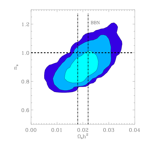
Figure 6: Constraints in the $\Omega_{b}h^{2}$ vs. $n_{s}$ plane from the combined BOOMERANG and COBE/DMR datasets. The likelihood at each point is computed by maximizing over the remaining five parameters. The shaded regions correspond to $68.3\%$, $95.4\%$ and $99.7\%$ confidence levels. The bound obtained from standard BBN is overlaid.

Since $n_{s}$ and $\tau_{C}$, the optical depth to the surface of last scattering, are also highly correlated, there is a noticeable difference between marginalization and maximization, as seen in Fig. 4. Increasing $\tau_{C}$ suppresses the high-$\ell$ power spectrum by a constant factor $\sim\exp{-2\tau_{C}}$, but leaves the lowest multipoles unaffected. This is similar to the effect of altering the spectral index, which changes higher multipoles with a longer “lever arm” with respect to the lower $\ell$. Because the likelihood functions peak for nearly all models at $\tau_{C}=0$, the maximization procedure effectively ignores $\tau_{C}>0$, whereas marginalization averages over the allowed values of $\tau_{C}$, accounting for the increase from 0.90 to 0.96. (If we restrict ourselves to $\tau_{C}=0$, we get $0.89^{+.09}_{-.08}$ with maximization, $0.92^{+.08}_{-.07}$ with marginalization.)

The values of the spectral index, the curvature and the cosmological constant affect the shape and the amplitude of the power spectrum of the matter distribution. The bandpower $\sigma_{8}^{2}$, giving the variance in (linear) matter fluctuations averaged in $8h^{-1}Mpc$ spheres, is often used to characterize the results of many large scale structure observations. In Lange et al. (2001), Jaffe et al. (2001) and B01, $\sigma_{8}\Omega_{m}^{0.56}$=$0.55^{+.02,+.11}_{-.02,-.08}$ was adopted, where the combination of Gaussian and top hat error bars were used to generate a wide distribution “weak” large scale structure prior to be imposed upon the CMB data. This compares with $\sigma_{8}\Omega_{m}^{0.5}\sim 0.50\pm 0.05$ estimated by Pen (1998) and a best fit value $\sigma_{8}\Omega_{m}^{0.47}\sim 0.56$ from Viana & Liddle (1999). We have computed $\sigma_{8}$ for each model in our database using the matter fluctuations power spectrum. From the likelihood analysis in the space ($\sigma_{8},\Omega_{m}$), we find the 1-sigma range $0.5\lower 2.15277pt\hbox{$\;\buildrel<\over{\sim}\;$}\sigma_{8}\lower 2.15277pt\hbox{$\;\buildrel<\over{\sim}\;$}0.8$ for $0.3\lower 2.15277pt\hbox{$\;\buildrel<\over{\sim}\;$}\Omega_{m}\lower 2.15277pt\hbox{$\;\buildrel<\over{\sim}\;$}0.7$. For the detailed application of the weak large scale structure prior of Lange et al. (2001), which also included a constraint on the shape of the power spectrum, see B01.

5 Discussion and Conclusions

We have analyzed the most recent results from BOOMERANG, and shown that there are a series of 5 features, 3 peaks with 2 interleaved dips, each of which is detected using a cosmological model independent method at $\sim 95\%$ or better confidence. Because BOOMERANG is able to achieve resolution in $\ell$-space of $\Delta\ell\sim 50$, with only $\sim 10\%$ (anti)-correlation between bins, the data determine the positions as well as the amplitudes of each of the features with reasonable precision.

The positions and amplitudes of the features are consistent with the results of the DASI experiment. A direct, cosmological model-independent comparison of the two experiments is made difficult by the lower $\ell$-space resolution of the DASI experiment. However, the two results can be accurately compared via a model-dependent analysis that takes millions of ${\cal C}_{\ell}$ shapes with very different peak/dip amplitudes and locations, weighted their peak and dip locations with the probability of the (normalized) shapes, and finds well-localized $\ell_{\rm p}$ and ${\cal C}_{\rm p}$ for each of the peaks and dips. The agreement between BOOMERANG and DASI using this method is very good, and completely consistent with the model-independent results. It will of course be of great interest whether the forecasts allowed by this model-dependent technique for the positions and amplitudes of the next peaks and dips will be borne out by even higher resolution observations.

The natural interpretation of this much-anticipated sequence of peaks and dips in ${\cal C}_{\ell}$ is that we are seeing phase-coherent pressure waves in the photon-baryon fluid at photon decoupling at redshift $\sim 1100$, expected in adiabatic models of structure formation, and which therefore the simplest inflation models give. This is certainly the most economical interpretation, especially since the locations within this paradigm correspond to widely-anticipated cosmological parameter choices, namely $\Omega_{tot}\approx 1$, $\Omega_{m}\sim 1/3$, $\Omega_{B}h^{2}\approx 0.02$, with a nearly scale invariant spectrum, $n_{s}\sim 1$. We have shown how well determined and robust these parameter values are to changes in the ${\cal C}_{\ell}$ database, in using likelihood maximization or Bayesian marginalization, and to using either the BOOMERANG or DASI ${\cal C}_{\ell}$s in conjunction with the DMR ${\cal C}_{\ell}$s.

Of course this does not clinch the case: the derived cosmological parameters could be quite different if we allowed ourselves much further freedom beyond a single slope to characterize the primordial spectrum. It could even be that the peaks and dips reflect early universe structures rather than sound wave structures. It is also possible that isocurvature modes with artful enough initial condition choices could mimic the simple adiabatic case (e.g. Turok, 1996). The detection of the associated polarization peaks and dips would rule out these more exotic possibilities. Although there are no glaring anomalies between theory and data at this stage requiring a revisit of basic CMB assumptions, the improved precision in this $\ell$-range that more sky coverage will give, and the extension to higher $\ell$ that other CMB experiments will give, could well reveal that our forecasts are wrong. Even with the current data, there is certainly room for other cosmological parameters not treated in our minimalist inflation databases, and such explorations are underway.

References

- Albrecht et al. (1996) Albrecht, A., Coulson, D., Ferreira, P. & Magueijo, J. 1996, Phys. Rev. Lett. 76, 1413
- Balbi et al. (2000) Balbi, A. et al 2000, Ap.J. 545 LX-LY, astro-ph 0054312
- Bond & Efstathiou (1987) Bond, J.R. & Efstathiou, G. 1987, Mon. Not. R. Astron. Soc. 226, 655
- Bond et al. (2000) Bond J.R. et al. 2001, Proc. IAU Symposium 201, astro-ph/0011378
- Bond, Jaffe, and Knox (1998) Bond, J.R., Jaffe, A.H. & Knox, L. 1998, Phys. Rev. D57, 2117
- Bond, Jaffe & Knox (2000) Bond, J. R., Jaffe, A. H., & Knox, L. 2000, ApJ 533, 19
- Bridle et al. (2000) Bridle S. et al. 2000, astro-ph/0006170
- Bucher et al. (2000) Bucher, M., Moodley, K. & Turok, N. 2000, astro-ph/0007360
- Burles et al. (2000) Burles, S., Nollett, K.M. & Turner, M.S. 2000, astro-ph/0010171
- de Bernardis et al. (1997) de Bernardis, P. et al. 1997, Ap.J., 480, 1
- de Bernardis et al (2000) de Bernardis, P. et al. 2000, Nature, 404, 955
- Dodelson & Knox (2000) Dodelson, S. and Knox, L. 2000, Phys. Rev. Lett. 84, 3523
- Efstathiou & Bond (1999) Efstathiou G. & Bond, J.R. 1999, Mon. Not. R. Astron. Soc. 304, 75
- Griffiths et al. (2001) Griffiths L. M., Melchiorri A., Silk J.I. 2001, Ap. J. Lett., in press, astro-ph/0101413
- Halverson et al. (2001) Halverson N.W. et al. 2001, astro-ph/0104489
- Hanany et al. (2000) Hanany, S. et al. 2000, ApJ, 545, L5
- Jaffe et al. (2001) Jaffe A., et al. 2001, Phys. Rev. Lett., 86, 3475
- Kamionkowski & Kosowsky (1999) Kamionkowski M. & Kosowsky A. 1999, Ann. Rev. Nucl. Part. Sci., 49, 77
- Kinney et al. (2000) Kinney W., Melchiorri A., Riotto A. 2000, preprint astro-ph/0007345
- Knox & Page (2000) Knox L. & Page L. 2000, Phys. Rev. Lett. 85, 1366
-
Knox (2000)
Knox L. 2000,
http://flight.uchicago.edu/knox/radpack.html - Lange et al. (2001) Lange A.E. et al. 2001, Phys. Rev. D 63, 042001, astro-ph/0005004
- Lee et al. (2001) Lee A.T. et al. 2001, astro-ph/0104459
- Mauskopf et al. (2000) P. D. Mauskopf et al. 2000, Ap.J 536, L59
- Melchiorri et al. (1999) Melchiorri A., et al., 2000, Ap.J.Lett. 536, L63
- Miller et al. (1999) A. D. Miller et al. 1999, Ap.J. 524, L1
- Netterfield et al. (2001) Netterfield C.B. et al. 2001, submitted to Ap.J., astro-ph/0104460
- Peebles et al. (1970) Peebles, P.J.E, and Yu, J.T. 1970, Ap.J. 162, 815
- Peebles et al. (2000) Peebles, P.J.E., Seager, S. and Hu, W. 2000, astro-ph/0004389
- Pen (1998) Pen, Ue-Li 1998, Ap.J. 498, 60
- Perlmutter et al. (1997) Perlmutter, S. et al. 1997, Ap. J. 483, 565; P.M. Garnavich et al. 1998, Ap.J. Letters 493, L53; S. Perlmutter et al. 1998, Nature 391, 51; A.G. Riess et al. 1998, Ap. J. 116, 1009
- Pryke et al. (2001) Pryke C. et al. 2001, astro-ph/0104490
- Sigurdson & Scott (2000) Sigurdson, K. and Scott, D. 2000, New Astronomy 5, 91
- Seljak & Zaldarriaga (1996) Seljak, U. & Zaldarriaga, M. 1996, Ap.J. 469, 437
- Silk & Wilson (1980) Silk J. & Wilson M. L. 1980, Physica Scripta, 21, 708
- Sunyaev & Zeldovich (1970) Sunyaev, R.A. & Zeldovich, Ya.B., 1970, Astrophysics and Space Science 7, 3
- Tegmark & Zaldarriaga (2000) Tegmark, M. and Zaldarriaga, M. 2000, astro-ph/0004393
- Turok (1996) Turok, N. 1996, Phys. Rev. Lett. 77, 4138
- Viana & Liddle (1999) Viana, P. & Liddle, A.R. 1999, M.N.R.A.S. 303, 535