Effects of SNe II and SNe Ia Feedback on the Chemo-Dynamical Evolution of Elliptical Galaxies

Abstract

We numerically investigate the dynamical and chemical processes of the formation of elliptical galaxies in a cold dark matter (CDM) universe, in order to understand the origin of the mass-dependence of the photometric properties of elliptical galaxies. Our three-dimensional TREE N-body/SPH numerical simulations of elliptical galaxy formation take into account both Type II (SNe II) and Type Ia (SNe Ia) supernovae (SNe) and follow the time evolution of the abundances of several chemical elements (C, O, Ne, Mg, Si, and Fe). Moreover we compare different strengths of SNe feedback. In combination with stellar population synthesis, we derive the photometric properties of simulation end-products, including the magnitude, color, half-light radius, and abundance ratios, and compare them with the observed scaling relations directly and quantitatively. We find that the extremely strong influence of SNe is required to reproduce the observed color-magnitude relation (CMR), where we assume each SN yields energy of $4\times 10^{51}$ ergs and that 90% of this energy is ejected as kinetic feedback. The feedback affects the evolution of lower mass systems more strongly and induces the galactic wind by which a larger fraction of gas is blown out in a lower mass system. Finally higher mass systems become more metal rich and have redder colors than lower mass systems. We emphasize based on our simulation results that the galactic wind is triggered mainly by SNe Ia rather than SNe II. In addition we examined the Kormendy relation, which prescribes the size of elliptical galaxies, and the [Mg/Fe]–magnitude relation, which provides a strong constraint on the star formation history.

1 Introduction

Despite the large variety in the internal dynamics and structures, elliptical galaxies follow the various scaling relations. These relationships are expected to contain valuable information about physical processes of their formation. For example, colors of elliptical galaxies strongly correlate with their luminosities (e.g., Sandage, 1972; Aaronson, Persson, & Frogel, 1981; Bower, Lucey, & Ellis, 1992a, b, hereafter BLE92a and BLE92b). This relation is usually called the color-magnitude relation (CMR). The CMR is conventionally interpreted as an effect of the galactic metallicity increasing with the mass (e.g., Faber, 1973; Dressler, 1984), although the age difference also contributes on the CMR possibly (Worthey, Trager, & Faber, 1996). This interpretation is supported by line index analysis of galaxies (Kuntschner & Davies, 1998; Kuntschner, 1998; Terlevich et al., 1999; Kuntschner, 2000) and slopes of CMRs observed in the intermediate redshift ($z\sim 0.8$) clusters (Kodama & Arimoto, 1997). The mass-metallicity sequence can be naturally explained by the galactic wind scenario (Larson, 1974) and reproduces the CMR very well, according to the previous studies employing the evolutionary method of population synthesis (e.g., Arimoto & Yoshii, 1987; Matteucci & Tornamb$\rm\grave{e}$, 1987; Gibson, 1997; Tantalo et al., 1998). In this scenario, galactic wind is induced progressively later in more massive galaxies owing to deeper potential and stellar populations in brighter galaxies are much more enhanced in heavy elements, leading to redder colors. However, these studies assumed a simple galaxy model which ignored the internal structure and complex star formation history in a forming galaxy.

Recently developed semi-analytic model (White & Rees, 1987; White & Frenk, 1991) makes it possible to describe some complex star formation histories, such as a star-burst induced by a coalescence of galaxies. This model is based on the hierarchical clustering scenario expected in the cold dark matter (CDM) cosmology. The formation and merging histories of dark matter halos are deduced by an extended Press-Schechter theory (Bower, 1991; Bond et al., 1991) or a cosmological N-body simulation. The model presumes that gas initially cools into a disk and forms stars inside the halo. A spheroidal stellar system is assumed to be formed by a major merger of two disk galaxies (Kauffmann, White, & Guiderdoni, 1993; Baugh, Cole, & Frenk, 1996). Kauffmann & Charlot (1998) showed by taking account of chemical enrichment that the CMR of elliptical galaxies is reproduced in their semi-analytic model with the assumption that the supernova feedback is much efficient. Although the recent semi-analytic models seem to succeed in explaining the observational properties of galaxies at various redshifts, they inevitably assumed a phenomenological model involving a number of parameters to describe the processes of radiative cooling, star formation and feedback within the galactic halo. Moreover, structures of the end-products could not be discussed, because there is no information about the dynamical history of gas and star components.

Numerical simulations are powerful tools to treat the complex physical processes in galaxy formation self-consistently. In recent works using three dimensional numerical simulations which calculate the dynamical and chemical evolution self-consistently, photometric properties of end-products were investigated in combination with the stellar population synthesis and compared to the observations directly (e.g., Bekki & Shioya, 1998, 1999; Contardo, Steinmetz, & Fritze-von Alvensleben, 1998; Mori, Yoshii, & Nomoto, 1999; Steinmetz & Navarro, 1999; Koda, Sofue, & Wada, 2000a, b; Navarro & Steinmetz, 2000; Kawata, 1999, 2001, hereafter K99, K01). In order to understand the connection between the observed scaling relations and the physical processes of the formation of elliptical galaxies, we investigate the dynamical and chemical evolution of elliptical galaxies in a cold dark matter (CDM) universe using the numerical simulation. In this paper we focus on understanding the origin of the CMR, i.e., how and what physical processes control the mass dependence of the photometric properties. To this end, we adopt the elliptical galaxy formation model of K99. This model is based on a semi-cosmological model proposed by Katz & Gunn (1991) and treats a collapse of a top-hat over-dense sphere which initially follows a Hubble flow expansion and has a solid-body rotation as an effect of the external tidal field. In addition this sphere includes small-scale density fluctuations expected in a CDM universe. The galaxy is built by merger of small clumps formed due to the small-scale fluctuations, i.e., a hierarchical clustering. K99 studied the evolution of a seed galaxy which has a slow rotation corresponding to a spin-parameter of $\lambda=0.02$ and showed that the end-product reproduces the observed properties of elliptical galaxies very well. Cosmologically, a small spin-parameter is preferred in a galactic halo collapsing at a high redshift (Heavens & Peacock, 1988). The reason for this is that higher peaks have a shorter collapse time; thus, they have less time to get spun up by the environmental tidal force. Moreover, a significant fraction of elliptical galaxies are considered to be the systems which had collapsed at high redshifts, according to the zero-point and tightness of the CMR at the intermediate redshift (e.g., Bower, Kodama, & Terlevich, 1998; van Dokkum et al., 2000). It is thus a natural supposition that some elliptical galaxies were formed in a halo collapsing at a high redshift and rotating slowly (e.g., Blumenthal et al., 1984). Although K99 studied the dynamical and chemical evolution of a galaxy with a fixed mass, we here examine the photometric properties of the end-products with different masses. We pay a particular attention to the supernovae feedback, which is one of the most difficult processes to model in the present-day numerical simulations, but considered to be a crucial determinant of the nature of the stellar population of the end-products. Therefore, we examine how the difference in the strength of the feedback affects the final CMR. In addition our numerical code takes account of the chemical and dynamical feedback of both Type II (SNe II) and Type Ia (SNe Ia) supernovae (SNe) and follows the evolution of the abundances of several chemical elements (C, O, Ne, Mg, Si, and Fe). We evaluate relative importance of two types of SNe, SNe II and SNe Ia, on the dynamical and chemical evolution. Since our numerical simulations naturally provide the information about the structure of end-products with enough spatial resolution, we compare simulation results not only with the observed CMR but also with the Kormendy relation, which prescribes the size of elliptical galaxies as a function of their luminosity. Due to self-consistent calculation of evolution of chemical elements abundances, we can also study the mass dependence of abundance ratios. Kuntschner (1998, 2000) studied early-type galaxies in the Fornax cluster, using the line indices analysis for high-quality data. He found that Fornax ellipticals are mainly old and also discovered a strong relation between [Mg/Fe] and the velocity dispersion (see also Trager et al., 2000b). Jørgensen (1999) studied Coma elliptical and obtained a strong correlation between [Mg/Fe] and not only the velocity dispersion but also the luminosity. Hereafter we call the correlation between [Mg/Fe] and the luminosity “[Mg/Fe]–magnitude relation”. Because Mg and Fe are mostly produced by SNe II and SNe Ia respectively and because SNe Ia have a longer delay than SNe II after formation of stars, these correlations give strong constraints on the star formation history of elliptical galaxies (Matteucci, Ponzone, & Gibson, 1998; Thomas, Greggio, & Bender, 1999). We examine the [Mg/Fe]–magnitude relation for the simulation end-products and compare it with the observation.

The plan for the remainder of this paper is as follows. The numerical method and the model used in this paper are described in Sections 2 and 3. We show the procedure to derive the photometric properties of the simulation end-products in Section 4. In Section 5, results of numerical simulations are presented and are compared with the observed global scaling relations. Our discussion and conclusions are given in Section 6.

2 The Code

Numerical simulations are performed using an update version of the code in K99 so that SNe Ia feedback is taken into account. Because we have already described the details of the code in K99, here we describe mainly the modelings of star formation and their feedback which are revised. Our code is essentially based on the TreeSPH (Hernquist & Katz, 1989; Katz, Weinberg, & Hernquist, 1996), which combines the tree algorithm (Barnes & Hutt, 1986) for the computation of the gravitational forces with the smoothed particle hydrodynamics (SPH: Lucy, 1977; Gingold & Mnoraghan, 1977) approach to numerical hydrodynamics. The dynamics of the dark matter and stars is calculated by the N-body scheme, and the gas component is modeled using the SPH. It is fully Lagrangian, three-dimensional, and highly adaptive in space and time owing to individual smoothing lengths and individual time steps. Moreover, it self-consistently includes almost all the important physical processes in galaxy formation, such as self-gravity, hydrodynamics, radiative cooling, star formation, supernova feedback, and metal enrichment.

The radiative cooling which depends on the metallicity (Theis, Burkert, & Hensler, 1992) is taken into account. The cooling rate of a gas with the solar metallicity is larger than that for a gas of the primordial composition by more than an order of magnitude. Thus, the cooling by metals should not be ignored in numerical simulations of galaxy formation (Käellander & Hultman, 1998; Kay et al., 2000).

2.1 Star Formation

We model star formation using a method similar to that of Katz (1992) and Katz, Weinberg, & Hernquist (1996). We use the following three criteria for star formation: 1) the gas density is greater than a critical density, $\rho_{\rm crit}=2\times 10^{-25}\ {\rm g\ cm^{-3}}$, i.e., $n_{\rm H}\sim 0.1{\rm cm^{-3}}$, following Katz, Weinberg, & Hernquist (1996); 2) the gas velocity field is convergent, ${\bf\nabla}\cdot\mbox{\boldmath$v$}_{i}<0$; and 3) the Jeans unstable condition, $h/c_{s}>t_{\rm g}$, is satisfied, here $h$, $c_{s}$, and $t_{\rm g}=\sqrt{3\pi/16G\rho_{\rm g}}$ are the SPH smoothing length, the sound speed, and the dynamical time of the gas respectively (see K99 for details). The Jeans condition was ignored in K99 and K01, because the gas whose density is higher than $\rho_{\rm crit}$ usually satisfies this condition. Since the Jeans unstable condition might be important in the low mass systems, we take it into account in this paper.

When a gas particle is eligible to form stars, its star-formation rate (SFR) is

$$\frac{d\rho_{*}}{dt}=-\frac{d\rho_{\rm g}}{dt}=\frac{c_{*}\rho_{\rm g}}{t_{\rm g}},$$ (1)

where $c_{*}$ is a dimensionless SFR parameter and $t_{\rm g}$ is the dynamical time, which is longer than the cooling timescale in the region eligible to form stars. This formula corresponds to the Schmidt law that SFR is proportional to $\rho_{\rm g}^{1.5}$. The value of $c_{*}$ controls the SFR with respect to the local gas density, namely star formation efficiency. When a large $c_{*}$ is assumed, many stars can be formed well before the system collapses completely, so that the effective radius of the final stellar system becomes large. In this paper we assume for simplicity that $c_{*}$ is constant irrespective of the mass of the system and calibrated $c_{*}$ so that model A2 defined in Section 3 could reproduce the observed Kormendy relation. Figure 5.2 shows the results of model A2 in the case of $c_{*}=1$ (cross) and $c_{*}=0.5$ (triangle just under the cross) respectively. We can see that $c_{*}=1$ leads to a little larger effective radius than the observed elliptical galaxies under the assumed distance modulus (see Section 5 for details). Although the difference in $c_{*}$ a little affects the other photometric properties which we examine in this paper (Fig. 5 and 5.3), finally we found that this effect is quite small, compared to difference in the strength of SNe feedback which we focus on in this paper. Consequently we set $c_{*}=0.5$. In addition the above critical gas density, $\rho_{\rm crit}$, is higher than that in K99 and K01. We also carried out a simulation with the same $\rho_{\rm crit}$ as K99 and found that this difference does not change the effective radius in model A2, because the gas density becomes higher than these densities very quickly once the system collapses. The difference in $\rho_{\rm crit}$ within this range does not affect our results.

We assume that the stars which are represented by a star particle are distributed according to the Salpeter (1955) initial mass function (IMF). The IMF by number, $\Phi(m)$, in each mass interval $dm$ is defined as

$$\Phi(m)dm=Am^{-(1+x)}dm,$$ (2)

where $x=1.35$ is the Salpeter index (this corresponds to an IMF by mass $\propto m^{-x}$) and the coefficient $A$ is determined by the normalization in the mass range $M_{\rm l}\leq m\leq M_{\rm u}$. We set $M_{\rm u}=60\ {\rm M_{\odot}}$ and $M_{\rm l}=0.4\ {\rm M_{\odot}}$ respectively.

2.2 The Feedback

We take account of the energy feedback and metal enrichment to the surrounding gas by SNe. We consider here both SNe II and SNe Ia. The simulation follows the evolution of the abundances of several chemical elements (C, O, Ne, Mg, Si, and Fe).

2.2.1 Type II Supernovae

For simplification, we assume that each massive star ($>10\ {\rm M_{\odot}}$) explodes as a type II supernova within the simulation time step in which it was born (instantaneous recycling). From equation (2) the number of SNe II in a new-born star particle of $m_{\rm s}\ {\rm M_{\odot}}$ becomes $N_{\rm SNeII}=9.26\times 10^{-3}m_{\rm s}$. The total stellar mass contributing to SNe II is $M_{\rm SNeII}=1.83\times 10^{-1}m_{\rm s}\ {\rm M_{\odot}}$ and the mass of $(M_{\rm SNeII}-1.4N_{\rm SNeII})\ {\rm M_{\odot}}$ is returned to the the surrounding gas, where the remnant mass is assumed to be $1.4\ {\rm M_{\odot}}$. In this process, a portion of the metals produced in the stars is also returned to the gas, leading to chemical enrichment. We use the stellar yields derived by Notomo et al. (1997a) who provide for SNe II the $i$-th heavy element mass, $M_{i,{\rm SNeII}}(m)$, produced in a star of main-sequence mass of $m$. Then the synthesized mass of SNe II in a new-born star particle of $m_{\rm s}\ {\rm M_{\odot}}$ for each element is calculated by

$$M_{i,{\rm SNeII}}=m_{\rm s}\int_{10\ {\rm M_{\odot}}}^{M_{\rm u}}M_{i,\rm SNeII}(m)m^{-(1+x)}dm\left/\int_{M_{\rm l}}^{M_{\rm u}}m^{-x}dm\right.\ {\rm M_{\odot}}.$$ (3)

Table 1 shows $M_{i,{\rm SNeII}}$ for each element. Here we assume that the heavy-element production from a star of 10 ${\rm M_{\odot}}$ is negligible, following Tsujimoto et al. (1995).

These mass, energy, and heavy elements are smoothed over the neighboring gas particles using the SPH smoothing algorithm. For example, when the $i$-th particle changes from gas to a star, the increment of the mass of the $j$-th neighbor particle due to explosion of the new-born star is given by

$$\Delta{M_{\rm SN,{\it j}}}=\frac{m_{j}}{\rho_{{\rm g},i}}{M_{\rm SN,{\it i}}}W(r_{ij},h_{ij}),$$ (4)

where

$$\rho_{{\rm g},i}=\langle\rho_{\rm g}(\mbox{\boldmath$x$}_{i})\rangle=\sum_{j\neq i}m_{j}W(r_{ij},h_{ij})$$ (5)

and $W(r_{ij},h_{ij})$ is an SPH kernel (see K99).

2.2.2 Type Ia Supernovae

Comparing the predicted nucleosynthesis products of SNe Ia and SNe II with the solar abundances of heavy elements and their isotopes, Tsujimoto et al. (1995) derived that the ratio of the total numbers of SNe Ia to SNe II is $N_{SNeIa}/N_{SNeII}=0.15$. If the progenitor of SNe Ia is a binary system one of which has a mass range of $m=3$-$8\ {\rm M_{\odot}}$, $N_{\rm SNeIa}/N_{\rm SNeII}$ is calculated by

$$\frac{N_{\rm SNeIa}}{N_{\rm SNeII}}=\frac{A_{\rm Ia}\int_{3\ {\rm M_{\odot}}}^{8\ {\rm M_{\odot}}}m^{-(1+x)}dm}{\int_{10\ {\rm M_{\odot}}}^{60\ {\rm M_{\odot}}}m^{-(1+x)}dm}.$$ (6)

Thus, we adopt $A_{\rm Ia}\sim 0.04$. Then the number of SNe Ia in a new-born star particle of $m_{\rm s}\ {\rm M_{\odot}}$ becomes $N_{\rm SNeIa}=1.52\times 10^{-3}m_{\rm s}$ and the ejected mass is assumed to be $A_{\rm Ia}$ times the total mass of stars whose mass is between 3 ${\rm M_{\odot}}$ to 8 ${\rm M_{\odot}}$, i.e., $M_{\rm SNeIa}=6.94\times 10^{-3}m_{\rm s}\ {\rm M_{\odot}}$. The nucleosynthesis prescriptions for SNe Ia are taken from Notomo et al. (1997b) as shown in Table 1. If SNe Ia occur in a binary systems with the above mass range, SNe Ia should have various lifetime depending on the main-sequence lifetime of a secondary star. Therefore, SNe Ia are expected to continuously occur for a long time once they take place in the most massive binary system (e.g., Greggio & Renzini, 1983). Moreover, most recently a new SNe progenitor scenario in which SNe Ia rate depends on the metallicity was suggested and it was shown that this scenario is suitable for the explanation of the observed chemical evolution in the solar neighborhood (Kobayashi et al., 1998). However, we fix the lifetime of SNe Ia to 1.5 Gyr for simplicity, following a result of Yoshii, Tsujimoto, & Nomoto (1996), who presented that the mean lifetime of the progenitors of SNe Ia is about 1.5 Gyr, based on the chemical evolution analysis in the solar neighborhood.

2.2.3 The Energy Feedback

One of the most difficult and most critical processes to model in galaxy formation simulations is the way in which the feedback from SNe affects the surrounding gas. Unfortunately, there is no well understanding of how it should be modeled. In a pioneering SPH simulation by Katz (1992) the energy feedback was implemented as deposition of purely thermal energy into the surrounding gas. Katz (1992) founds that this form of energy feedback is rather inefficient; the high densities of typical star-forming regions imply short cooling timescales that minimize the hydrodynamical effects of the feedback energy input. In real star-forming systems SNe are largely responsible for the multi-phase structure of the interstellar medium (e.g., Mckee & Ostriker, 1977). Although they are associated with the cool and dense gas clouds, they can deposit much of their energy in a hot and low density wind. A seminal attempt at representing this multi-phase interstellar medium (ISM) has been carried out by Yepes et al. (1997) and recently Hultman & Pharasyn (1999) have adapted the Yepes et al. model to SPH simulations. However, they had to make a number of assumptions about the physics of the ISM and their models are not truly multi-phase, because different phases are treated as a dynamically single entity. Another implementation assumed that the feedback region around newly born stars evolves adiabatically until the multiple SNe II phase ends (e.g., Mori et al., 1997; Thacker & Couchman, 2000). Although this model is somewhat artificial, it can provide strong effects on the formation of dwarf galaxies (Mori et al., 1997).

While a number of models for energy feedback are proposed by previous authors as mentioned above, we adopt here the model proposed by Navarro & White (1993). This model assumes for simplicity that the energy produced by SNe affects only the temperature and velocity field of the surrounding gas and its effect is implemented by increasing the internal and kinetic energy of the gas neighbors of each star particle by amount corresponding to the energy released by SNe. Thus, when $i$-th new born star particle ejects the energy of $E_{{\rm SN},i}$ and deposits the energy of $\Delta E_{{\rm SN},j}$ in the $j$-th neighbor gas particle, the velocity of the $j$-th gas is altered by $\Delta v_{{\rm SN},j}$, which is calculated from

$$f_{v}\Delta E_{{\rm SN},j}=f_{v}E_{{\rm SN},i}\frac{m_{j}}{\rho_{{\rm g},i}}W(r_{ij},h_{ij})=m_{j}(\mbox{\boldmath$v$}_{j}\cdot\Delta\mbox{\boldmath$v$}_{{\rm SN},j}+\frac{1}{2}\Delta v_{{\rm SN},j}^{2}),$$ (7)

where $\mbox{\boldmath$v$}_{j}$ is the relative velocity to the $i$-th star, $\Delta\mbox{\boldmath$v$}_{{\rm SN},j}$ is a velocity perturbation directed radially from the $i$-th star, and $f_{v}$ is an input parameter which controls the fraction of the available energy to perturb the gas velocity field. The rest of the energy of the SNe, $(1-f_{v})\Delta E_{{\rm SN},j}$, contributes to increase the internal energy of $j$-th gas. When the term of $\mbox{\boldmath$v$}_{j}\cdot\Delta\mbox{\boldmath$v$}_{{\rm SN},j}$ is assumed to be zero approximately (Navarro & White, 1993), the magnitude of the $\Delta\mbox{\boldmath$v$}_{{\rm SN},j}$ is then simply

$$\Delta v_{\rm SN,{\it j}}^{2}=2\frac{f_{v}\Delta E_{\rm SN,{\it j}}}{m_{j}}.$$ (8)

This model is consistent with the model of Katz (1992), in which $f_{v}=0$. The amount of effects of the energy feedback on forming galaxies depends quite strongly on the value of $f_{v}$. It is known that the kinetic feedback affects the history of star formation more strongly than the thermal feedback which quickly dissipates due to the radiative cooling in the high density region where stars can form (Navarro & White, 1993). Thus, $f_{v}$ controls the strength of the effect of SNe.

We assume that each SN yields energy of $\epsilon_{SN}\times 10^{51}$ ergs. According to high resolution 1D simulations of SN remnant in Thornton et al. (1998), 90 % of an initial SN energy is lost in radiation in its early expansion phase, which is not resolved in our simulations. However, an initial SN energy has not been established quantitatively yet. Therefore, we consider the available SN energy as a free parameter.

In our code, there are two parameters to control the strength of the effect of SNe. To examine the effect of the difference in the strength of the energy feedback, we carry out the simulations adopting two extreme sets of these parameters, namely $(\epsilon_{SN},f_{v})=(0.1,0)$ and $(\epsilon_{SN},f_{v})=(4,0.9)$. The former means a minimum feedback model, corresponding to the result of Thornton et al. (1998) when an initial SN energy $10^{51}$ ergs is assumed. The latter provides a feedback strong enough to reproduce the observed CMR as shown later.

3 The Model

Using the above code, we calculate the following semi-cosmological model which is almost the same as the one in K99. We consider an isolated sphere, as a seed galaxy, on which small-scale density fluctuations corresponding to a CDM power spectrum are superimposed. Here, we use Bertschinger’s software COSMICS (Bertschinger, 1995) in generating initial density fluctuations. To incorporate the effects of fluctuations with longer wavelengths, the density of the sphere has been enhanced and a rigid rotation corresponding to a spin parameter, $\lambda$, has been added. The initial condition of this model is determined by the following four parameters: $\lambda$, $M_{\rm tot}$, $\sigma_{\rm 8,in}$, and $z_{\rm c}$. The spin parameter is defined by

$$\lambda\equiv\frac{J|E|^{1/2}}{GM_{\rm tot}^{5/2}},$$ (9)

where $J$ is the total angular momentum of the system, $E$ is the total energy, and $M_{\rm tot}$ is the total mass of this sphere, which is composed of dark matter and gas; $\sigma_{\rm 8,in}$ is the rms mass fluctuation in a sphere of radius $8\ h^{-1}$ Mpc, which normalizes the amplitude of the CDM power spectrum; $z_{\rm c}$ is the expected collapse redshift. If the top-hat density perturbation has an amplitude of $\delta_{i}$ at the initial redshift, $z_{i}$, we obtain $z_{\rm c}=0.36\delta_{i}(1+z_{i})-1$ approximately (e.g., Padmanabhan, 1993). Thus, when $z_{\rm c}$ is given, $\delta_{i}$ at $z_{i}$ is determined.

K99 found that the seed galaxy which has a slow rotation corresponding to $\lambda=0.02$ and the small-scale density fluctuations evolves into an elliptical-like system using the similar numerical simulation to that of this paper. This spin parameter is close to the minimum value possible in the CDM universe, according to the results of N-body simulations (Barnes & Efstathiou, 1987; Warren et al., 1992). In this paper we adopt this elliptical galaxy formation scenario. The main purpose of this paper is to study the evolution of seed galaxies with different masses. In addition we consider that the strength of feedback is crucial to give rise to mass-dependent evolution process. Thus, we simulate the evolution of the seed galaxies with the total mass between $8\times 10^{12}$ and $1\times 10^{11}$ ${\rm M_{\odot}}$, using the two codes with different strength of the SNe feedback as mentioned above. Parameters in each model are summarized in Table 2. Each model is labeled, for example, model ’A1’, according to the total mass and the strength of the SNe feedback. Models A have $(\epsilon_{SN},f_{v})=(0.1,0)$, whereas $(\epsilon_{SN},f_{v})=(4,0.9)$ in models B. The number in the model name represents the total mass of the seed galaxy. Hereafter we refer to the mass sequence from model A1 (B1) to model A4 (B4) simply as “model A (B)”. In all the models, we fix $\sigma_{\rm 8,in}=0.5$ and $z_{c}=3.5$.

Our simulations assume a flat universe ($\Omega=1$) with a baryon fraction of $\Omega_{\rm b}=0.1$ and a Hubble constant of $H_{0}=50\ {\rm km\ s^{-1}\ Mpc^{-1}}$. We carry out each simulation using 9171 particles for gas and dark matter respectively. The mass and spatial resolutions for each model are shown in Table 2. We simulate the evolution of each model from $z_{i}=40$ to $z=0$. The morphological evolutions of all the models are similar to the evolutions seen in Figure 1 of K99 and K01. Finally, nearly spherical stellar systems are formed at $z=0$ in all the models.

4 Data Analysis

To compare simulation results with the observational data of nearby elliptical galaxies directly, we have to deduce photometric properties of simulation end-products at $z=0$ for various models. We use the same procedures as K01. Here we briefly describe the procedure to derive the photometric properties from simulation results. For this purpose, we show the analysis for model A2 as an example.

In our simulations, the stellar particles contain the information about their age and metallicity due to the self-consistent calculation of the chemical and dynamical evolution. By means of the population synthesis, we can derive the photometric properties of the stellar system from this information. Here, the spectral energy distribution (SED) of each stellar particle is assumed to be that of a single stellar population (SSP) that means a coeval and chemically homogeneous assembly of stars. Since the observational data with which our results should be compared provide the luminosity distribution projected to a plane, we have to derive the projected distribution of SED from the three dimensional distribution of stellar particles. Finally, we obtain the projected images as shown in Figure 5 of K01. Then the flux of each stellar particle is smoothed using a gaussian filter with the filter scale of 1/4 of the softening length of the stellar particle. These images provide quite similar information to the imaging data obtained in actual observations. Thus we can obtain various photometric properties from these images in the same way as in the analysis of observational imaging data. In the following analysis, we use the images similar to the one displayed in Figure 5 of K01, but employing a 1001 $\times$ 1001 pixel mesh to span the squared region with 100 kpc on a side.

The $B$ (upper panel) and $V$ (lower panel) band surface brightness profiles in the $x-y$ projections for models A2 (left) and B2 (right). The solid lines denote the $r^{1/n}$ law best-fit for the data plotted as the solid symbols. The fitting parameters are shown in the lower left corner of each panel. The error bars are shown only for the solid symbols and correspond to the standard deviation (see text for details).

In this paper, we use the data of SSPs of Kodama & Arimoto 97 model (Kodama, 1997; Kodama & Arimoto, 1997). Kodama & Arimoto 97 model supplies the database of SSPs with two types of IMF: ($x$, $M_{\rm u}$, $M_{\rm l}$) = (1.35, 60, 0.1) and ($x$, $M_{\rm u}$, $M_{\rm l}$) = (1.1, 60, 0.1) in the definition of Section 2.1. We adopt the data of SSPs with the IMF of ($x$, $M_{\rm u}$, $M_{\rm l}$) = (1.35, 60, 0.1), while we use the IMF of ($x$, $M_{\rm u}$, $M_{\rm l}$) = (1.35, 60, 0.4) in the numerical simulations. We confirmed that the photometric properties presented in this paper are hardly changed, when we employ another dataset of SSPs with the IMF of ($x$, $M_{\rm u}$, $M_{\rm l}$) = (1.1, 60, 0.1). A shallower IMF has a similar fraction of massive stars to the Salpeter IMF ($x=1.35$) whose lower mass limit, $M_{l}$, is a little higher. Therefore, our use of the IMF of ($x$, $M_{\rm u}$, $M_{\rm l}$) = (1.35, 60, 0.1) is justified.

The left panels of Figure 4 shows the surface-brightness profiles for model A2 in the $B$ and $V$ bands obtained by setting the annuli of various radii in each band image. The error bars show the standard deviation in each annulus. We set the width of each annulus to half the softening length. Since the error is calculated in the flux, like $\sigma_{f_{B}}^{2}=<f_{B}^{2}>-<f_{B}>^{2}$, the error in the magnitude is defined, using the Taylor expansion, as

$$\sigma_{M_{B}}=2.5\left(\frac{\sigma_{f_{B}}}{<f_{B}>\ln(10)}-\frac{\sigma_{f_{B}}^{2}}{2<f_{B}>^{2}\ln(10)}\right).$$ (10)

These surface brightness profiles are in excellent agreement with the Sersic ($r^{1/n}$) law (Sersic, 1968),

$$I(r)=I_{e}10^{\{-b_{n}[(r/r_{{\rm e}})^{1/n}-1]\}},$$ (11)

where we adopt $b_{n}=0.868n-0.142$, so that the effective radius, $r_{e}$, equals the half light radius in the range $0.5\leq n\leq 16.5$ (Caon, Capaccioli, & D’Onofrio, 1993) and $I_{e}$ is the surface brightness at $r_{e}$. This corresponds to the de Vaucouleurs ($r^{1/4}$) law (de Vaucouleurs, 1948), when $n=4$. The solid lines in Figure 4 show the best-fits in applying equation (11). In fitting, we use the data with $\mu_{B}<27\ {\rm mag\ arcsec^{-2}}$ irrespective of the observed band. The best-fit parameters are shown in the lower left corner of each panel in Figure 4.

Color (top), luminosity weighted metallicity (2nd), luminosity weighted age (3rd), and [Mg/Fe] (bottom) gradients in the $x-y$ projection for models A2 (left) and B2 (right). The solid lines show the best-fit linear relations for the data plotted as the solid symbols. The gradients in best-fit lines are shown in the lower left corner of each panel. The error bars are shown only for the solid symbols in top and 2nd panels and for the data of $r<5$ kpc in 3rd and bottom panels.

The left panels of Figure 4 shows the color, metallicity, and age gradients for model A2. The color gradients are obtained by setting annuli of various radii in the $B$ and $R$ band images and subtracting the $R$ band magnitude from the $B$ band magnitude in each annulus. We made the projected images also for the metallicity and age, and obtained their radial profiles. Points indicate the average value in each annulus in the $x$-$y$ projections. The width of each annulus is set to half the softening length. The error bars show the standard deviation in each annulus. The error in the color is written as $\sigma_{B-R}=\sqrt{\sigma_{M_{B}}^{2}+\sigma_{M_{R}}^{2}}$. The profiles of color and metallicity [defined as $\log(Z/Z_{\odot})$] are fitted by linear regression. In fitting, we excluded the data at radii less than the softening length and greater than the radius at which the $B$ band surface brightness is $\mu_{B}=24.5\ {\rm mag\ arcsec^{-2}}$ (open symbols in Fig. 4), because the inner region is affected by the smoothing of gravitational forces whereas the number of particles within an annulus is too small in the outer region. The best-fit gradients are shown in the lower left corner of each panel in Figure 4 and also in Table 3. The data obtained from the simulation results have large errors leading to large errors in the calculated gradients. However negative gradients are clearly seen in colors and metallicity, i.e., the color (metallicity) at the center is redder (higher) than that in the outer region. Although we show only a luminosity weighted metallicity to compare with the observational data, the metallicity gradient weighted by the luminosity is slightly steeper than that weighted by the mass in all the models. It is known that a typical elliptical galaxy has $\Delta(B-R)/\Delta\log(r)=-0.09\pm 0.02$ (Peletier et al., 1990) and $\Delta\log(Z/Z_{\odot})/\Delta\log(r)=-0.30\pm 0.12$ (Kobayashi & Arimoto, 2000, and references therein). Although the gradients obtained from the simulation results have large errors, the median gradients of both color and metallicity for model A2 are steeper than those observed. We can see that the color gradients are caused by the metallicity gradients, because the age is equally old irrespective of the radius. The radial profile of the age has a slightly positive gradient. This positive gradient means that star formation persists over longer time in the inner region than in the outer region, due to dissipative infall of gas. Since the residual gas is polluted by past star formation, metal rich stars are formed in the central region where the duration of star formation is long (K99). This is the origin of the color and metallicity gradients. Recent observations using the metal absorption lines provide no (for ellipticals) or positive (for S0s) gradients of the age (Kuntschner, 1998). Since the age gradient in Figure 4 is too shallow, this gradient seems not to be detected in the current observations using the absorption lines.

Comparison of the effective radius (left) and total magnitude (right) derived by different methods. The upper panels compare the value derived from the $r^{1/n}$ law fitting in the $x$-$y$ projection with that in the $x$-$z$ projection. The lower panels compare the value derived from the $r^{1/n}$ law fitting (square) with the value derived from the large aperture photometry (circles) in the $x$-$y$ projection (see text for details). The open (solid) symbols indicate the value for model A (B).

We show the surface-brightness profiles and the color, metallicity, and age gradients for model B2 in the right panels of Figures 4 and 4 in order to evaluate the effect of the difference in the strength of the SNe feedback on these profiles and gradients. We analyzed these profiles and gradients also for the other models. Table 3 summarizes the results. In Table 3, we can see that the strong feedback of model B leads to a small $n$ in surface-brightness profiles and a shallow slope in color and metallicity gradients, compared to the ones of model A. Moreover, with decreasing mass of the system, $n$ decreases and the color and metallicity gradients becomes shallower in model B. In other words, the strong feedback affects these profiles and gradients more severely in lower mass systems. Similar results are obtained in Carlberg (1984a); Mori, Yoshii, & Nomoto (1999). The mass dependence of $n$ is consistent with the correlation between $n$ and luminosity in the observed elliptical galaxies qualitatively (Caon, Capaccioli, & D’Onofrio, 1993). On the other hand, there is no correlation between the observed color and metallicity gradients and the luminosity in luminous elliptical galaxies (Peletier et al., 1990; Kobayashi & Arimoto, 2000, and reference therein), and in less luminous elliptical galaxies ($M_{B}>-19$) there is still a large uncertainty (e.g., Vader et al., 1988).

The global photometric properties, such as the total luminosity, the colors, and the effective radius, are also obtained from the projected image data. In this paper, we focus on the CMR, the Kormendy relation, and the [Mg/Fe]–magnitude relation. Thus we have to analyze the total magnitude, the color, the effective radius, and [Mg/Fe] using the projected images. The total magnitude and the effective radius can be derived in two different ways. One method is to fit the surface brightness profile to the $r^{1/n}$ law (eq. [11]). This fitting formula directly provides the effective radius, and the integration from the center to the effective radius gives half the total luminosity. The other method is to assume that the aperture photometry with a sufficiently large aperture provides the total value. We assume that the luminosity derived with the 99 kpc aperture is the total luminosity. Then the effective radius is defined as the radius within which half the total luminosity is contained, and calculated by counting the luminosity from the center in the projected images. Throughout this paper we set the center to the position of a pixel which has the maximum $V$ band luminosity. Figure 4 compares the effective radius and the total magnitude derived by the different methods. These panels show that there is no systematic difference. Moreover Figure 4 indicates that the total magnitude and the effective radius do not depend on the direction of the projection. It means that the end-products are nearly spherical and the luminosity profiles are well approximated by the $r^{1/n}$ law (see also Figs. 4). Finally, we use the former method in the following discussion. Table 3 shows the total magnitude in the $B$, $V$, and $K$ bands and the effective radius in the $V$ and $K$ bands for each model. These data are derived from the fitting of the luminosity profiles in the $x$-$y$ projections and used in the next section.

In observation of elliptical galaxies, colors and [Mg/Fe] are usually obtained using a fixed aperture. Table 4 shows the $U-V$ and $V-K$ colors and [Mg/Fe] for each model. In the next section, we will compare the colors and [Mg/Fe] of the simulation end-product in each model with the observed values measured by BLE92a and Trager et al. (2000a). The values in Table 4 have been obtained by the analysis using the same aperture as BLE92a and Trager et al. (2000a). We made the projected image also for the luminosity weighted abundance of Mg and Fe, and analyzed the ratio of the mean abundance of Mg to that of Fe within the aperture.

The comparison of $V/\sigma$ for the simulation end-products and for galaxies in the Virgo and Coma clusters (small dots, Davies et al., 1983). The triangles (circles) connected by dotted (solid) lines indicate the $V/\sigma$ of model A (B).

Due to calculating dynamical evolution, we can analyze the dynamical properties of end-products. K01 showed that the elliptical galaxy formation model used in this paper leads to a small ratio of the rotational velocity to the velocity dispersion ($V/\sigma$), which is consistent with the observed $V/\sigma$ in bright elliptical galaxies. The observed $V/\sigma$ in elliptical galaxies increases with decreasing luminosity (Davies et al., 1983). Now we consider the galaxies with different masses, we analyzed $V/\sigma$ for all the models, to examine the mass dependence of $V/\sigma$. Figure 4 shows $V/\sigma$ against the B band absolute magnitude. In model A, $V/\sigma$ increases slightly with decreasing luminosity, like the tendency of the observational data. On the other hand, the strong feedback of model B seems to lead to a low $V/\sigma$, compared to the one of model A, in low mass systems. However, $V/\sigma$ of simulation end-products could not be measured accurately, because their rotation curves do not provide a clear flat shape, owing to their slow rotation and a poor spatial resolution of numerical simulation. In other words, $V/\sigma$ indicated in Figure 4 has ambiguity. Thus we conclude that all the models provides a small $V/\sigma$ around $0.1\sim 0.5$ irrespective of the luminosity or the feedback model. Our model cannot explain the existence of less luminous elliptical galaxies with a large $V/\sigma$, especially in model B, tough the observed $(V/\sigma)$s for less luminous galaxies have a broad range. We suppose that these systems might be formed from another initial condition, e.g., with a larger $\lambda$ or a smaller $\sigma_{\rm 8,in}$ (K01). This analysis made it clear that the final stellar systems which we focus on have a small $V/\sigma$ and are supported mainly by random motions in terms of kinetics. In the following sections, we concentrate on the photometric properties.

5 Global Scaling Relation

The photometric properties of the simulation end-products at $z=0$ which are derived by the data analysis described in Section 4 are compared with the observed global scaling relations of elliptical galaxies in this section. We first compare the simulation results with the observational data in the color versus magnitude diagram. Next we discuss the sizes of the simulation end-products, comparing them with the observed Kormendy relation. Finally we examine the correlation between the total magnitude and the abundance ratio of Mg to Fe, i.e., the [Mg/Fe]–magnitude relation, which is sensitive to the star formation history.

The comparison of the CMRs for the simulation end-products and the Coma cluster galaxies (small dots, BLE92a) in the aperture of 5 kpc. The triangles (circles) connected by dotted (solid) lines indicate the CMRs of model A (B). The dashed line shows the CMR fitted to the Coma cluster galaxies (BLE92b). The cross denotes the results of the same model as model A2 but with $c_{*}=1$ (see Section 2.1).

5.1 The Color–Magnitude Relation

We construct the CMRs in model A and B. Comparing model A with model B, we study the effect of the difference in the strength of the SNe feedback. Figure 5 shows the comparison of the simulation end-products and the observed galaxies in the Coma cluster in the $V-K$ and $U-V$ CMR. The data for galaxies in the Coma cluster are the observed CMR of BLE92a. Since there is no difference between S0s and ellipticals in the scaling relations which we discuss, we do not distinguish S0s from ellipticals. BLE92a supplies the $U-V$ and $V-K$ colors which refer to an aperture size of 11 arcsec and the $V$ band total magnitude derived from a combination of their data and the literature. Throughout this paper we adopt the distance modulus of the Coma cluster of $m-M=34.7$ mag; the Virgo distance modulus is $m-M=31.01$ (Graham et al., 1999) and the relative distance modulus of the Coma with respect to the Virgo is $m-M=3.69$ (BLE92b). This gives the luminosity distance of 87.1 Mpc for the Coma. We assume that the angular diameter distance equals the luminosity distance, because the redshift of the Coma cluster ($z\sim 0.023$) is nearly zero cosmologically. Then the aperture size of 11 arcsec at the distance of the Coma cluster corresponds to $\sim$ 5 kpc. The data for simulation end-products are tabulated in Tables 3 and 4. Although model A has a tendency that smaller galaxies have a bluer color, the slope is too shallow to reproduce the observed slope of the CMR in the Coma cluster. On the other hand, the slope of model B is steeper than that of model A, and model B well reproduces not only the slope but also the zero-point of the observed CMR. The success of model B is owing to the action of mass-dependent galactic wind as shown later in detail.

The CMRs for the simulation end-products in the 99 kpc aperture. The triangles (circles) connected by dotted (solid) lines indicate the results of model A (B). The dashed lines are the same as that in Figure 5.

The slope of model A is just an aperture effect. Elliptical galaxies have a color gradient that the color at the center is redder than that in the outer regions (e.g., Peletier et al., 1990) and the end-products in our simulations also have gradients (Fig. 4 in Section 4). Thus the color within a fixed aperture provides the color in a more central region for larger galaxies, and the color of large galaxies becomes redder than that of small galaxies even if the mean color of the whole galaxy is the same between the large and small galaxies. Figure 5.1 shows the CMR for the mean color within the aperture of 99 kpc, which covers almost the whole galaxy in all the models which we examined. The mean color of the whole galaxy in model A stays nearly constant when the mass varies. Hence the slope of model A in Figure 5 is caused only by the smallness of the aperture size. On the other hand, model B shows a significant slope even when a large aperture size is specified as shown in Figure 5.1. Aperture effect cannot be ignored when we discuss the CMR observed in an aperture of a small size. Unfortunately, accurate colors evaluated within various apertures have never been provided from any observations. Recently Scodeggio (2001) showed that the CMR derived using color measurements within the effective radius is significantly flatter than those based on fixed-aperture color measurements. Unfortunately, the photometric accuracy of their data was not good enough to derive an accurate CMR. We would like to stress that an observation in apertures of various sizes is quite important in understanding not only the CMR but also the color gradients in elliptical galaxies.

The metallicities (upper panel) and ages (lower panel) against the absolute $V$ band magnitude for each model. The triangles (circles) connected by dotted (solid) lines indicate the results of model A (B). The open (solid) symbols denote the values evaluated in the 5 kpc (99 kpc, spread over almost the whole galaxy) aperture.

There are two equally plausible interpretations of the CMR (Worthey, 1994). The sequences of colors and line strengths among elliptical galaxies can almost equally well be attributed to either age difference or metallicity difference. In the simulation this degeneracy can be broken completely, because we can directly analyze the metallicity and age in the simulation end-products. Figure 5.1 shows the metallicity and age for each model. Here the metallicity and age mean the luminosity weighted value. The age is very old irrespective of the models and the aperture. The metallicity slope exhibits a similar behavior to the color as a function of the luminosity. Model A has a weak slope in the metallicity–magnitude diagram of Figure 5.1 when the aperture size is 5 kpc, though the slope almost vanishes when the 99 kpc aperture is used. On the other hand, model B shows a significant slope irrespective of the aperture size, although a large aperture size leads to a shallower slope. Thus it is concluded that the slope of CMR in Figure 5 is caused solely by the effect of the metallicity.

Time variations of the event rate of SNe II (normal lines) and SNe Ia (thick lines) for all the models.

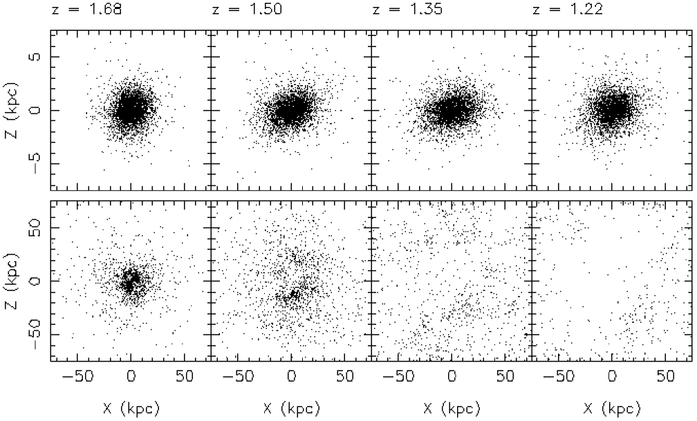
Figure 1: Time evolution of the system in model B4. The upper and lower panels shows the distributions of stellar particles and gas particles respectively. Upper (lower) panels show the $x$-$z$ projection of the particles and measure 15 (150) kpc across.

As a result, model B succeeds in reproducing the CMR by causing a decrease in the metallicity of the stellar contents for low-mass systems. On the other hand, model A completely fails. To see the origin of this difference, we examine the star formation history for each model. Figure 5.1 shows the histories of SNe II and SNe Ia event rates normalized by the total mass of the system. In our simulations, the histories of SNe II events completely trace those of star formation, because we assume the instantaneous recycling (see Section 2.1 for details). On the other hand, SNe Ia occur 1.5 Gyr behind SNe II. We can clearly see that in model B star formation abruptly ceases around $t=2.5\sim 3$ Gyr ($z=2\sim 1.7$). The dynamical evolution of the system clearly demonstrates that this is caused by the so-called galactic wind. Figure 1 which shows the morphological evolution of model B4. Around $z\sim 1.7$, gas particles begin to blow out from the stellar system, i.e., the galactic wind occurs. All the gas particles overcome the binding energy of the dark matter and stars, and escape from the system. In addition we found that the mass fraction of the ejected gas increases with decreasing mass of the system in model B, as seen in Figure 5.1. The ejected gas mass in Figure 5.1 is defined as the total mass of all the gas particles whose galactocentoric radius is greater than 20 kpc. Since the ejected gas cannot contribute to the further metal enrichment, a higher mass system suffers from more enhancement in heavy elements. This mass dependence of the mass fraction of the gas ejected by the galactic wind is the origin of the metallicity–magnitude relation shown in Figure 5.1, which in turn causes the CMR shown in Figure 5. There is little difference models B1 and B2 in Figure 5.1. In this luminosity range, the aperture effect is dominant factor in explaining the observe slope. However, the metallicity–magnitude relation caused by the galactic wind is essential in order to reproduce the global CMR in the observed luminosity range.

It is notable that the galactic wind occurs immediately after SNe Ia ignite. It is clearly shown that SNe Ia are important for the galactic wind. The event rate of SNe Ia exceeds that of SNe II after the peak of star formation. SNe Ia occur when the gas is exhausted by star formation and the gas density becomes low. Thus SNe Ia can strongly affect the evolution of the residual gas.

On the other hand, Figure 5.1 shows that almost all the gas is exhausted by $z=0$ irrespective of the mass of the system in model A. As a consequence, model A fails to reproduce the observed CMR. The difference in results of models A and B is the strength of the effect of SNe. As a result, a strong effect of the SNe feedback like the one included in model B is required to explain the observed CMR. Moreover we can clearly see from the results of model B that the mass fraction of the gas ejected by the galactic wind depends on the mass of the system and that SNe Ia play a quite important role in the outbreak of galactic wind.

The ratio of the ejected gas mass ($M_{\rm g,GW}$) at $z=0$ to the initial gas mass ($M_{\rm g,ini}$). The triangles (circles) connected by dotted (solid) lines indicate the data of model A (B). Here, the ejected gas is defined as the sum of all the gas particles whose galactocentoric radius is greater than 20 kpc.

5.2 The Kormendy Relation

Numerical simulations have a strong advantage over pure chemical evolution studies and semi-analytic models of galaxy formation in that simulations can provide information about the structure of the end-products. Owing to this advantage, we can discuss the scaling relation which prescribes the size of the elliptical galaxies, i.e., the Kormendy relation. Figure 5.2 displays the comparison of the Kormendy relations for the simulation end-products and the Coma cluster galaxies both in the $V$ and $K$ bands. We refer to the data of the Coma cluster galaxies of Pahre (1999). When we derive the absolute magnitude and the effective radius in the kpc unit from the data set in Pahre (1999), we assume the same distance modulus as mentioned above. In Figure 5.2, both models have a tendency that higher mass galaxies have larger effective radii, which is qualitatively consistent with the Kormendy relation for the observed elliptical galaxies. However the slope is too shallow in both models to consistent with the observed relation quantitatively. In particular, the slope of model B is much shallower than that of model A. This is due to the expansion of the low mass systems induced by the strong feedback. It is concluded that the strong feedback which is required to explain the observed CMR is unsuitable for explaining the Kormendy relation. The failure in reproducing the Kormendy relation poses a serious problem to the galactic wind scenario.

The comparison of the Kormendy relations for the simulation end-products and the Coma cluster galaxies (small dots, Pahre, 1999) in the $V$ (upper panel) and $K$ (lower panel) bands. The triangles (circles) connected by dotted (solid) lines indicate the data for model A (B). The cross denotes the results of the same model as model A2 but with $c_{*}=1$ (see Section 2.1).

5.3 The [Mg/Fe]–Magnitude relation

Our numerical code takes account of both SNe II and SNe Ia, and follows the evolution of the abundances of several chemical elements (C, O, Ne, Mg, Si, and Fe). Therefore we can examine the abundance ratio of chemical elements in the simulation end-products. Observational data indicate that [Mg/Fe] correlates with the luminosity, i.e., the [Mg/Fe]–magnitude relation (see also Section 1). We compare the [Mg/Fe]–magnitude relation for the simulation end-products with the observational data of local field and group elliptical galaxies. We use the observational data of [Mg/Fe] in Trager et al. (2000a) and the absolute B band magnitudes in Trager et al. (2000b). Trager et al. (2000a) derived [Mg/Fe] in the $r_{e,B}/2$ and $r_{e,B}/8$ apertures, using an extension of the Worthey (1994) models that incorporates nonsolar line-strength response functions by Tripicco & Bell (1995). We use the data for model 4 of Trager et al. (2000a), which is the most successful model according to their paper. In Figure 5.3 we compared the $r_{e,B}/2$ aperture data with [Mg/Fe] for the simulation end-products in the $r_{e,B}/2$ aperture. Since all the models do not reproduce the observed effective radius as shown in Section 5.2, the physical aperture size in all the models is not consistent with that applied in the observed galaxies with the same luminosity. Fortunately, the observed gradient of [Mg/Fe] is quite weak in these samples according to Trager et al. (2000a). On the other hand, Figure 4 shows the [Mg/Fe] gradients for models A2 and B2. Although there is a little gradient of [Mg/Fe] in the simulation results of model A, the gradient becomes shallower within the effective radius irrespective of models. Thus the difference in the aperture size is not so important in this case. The observed data show a clear tendency that [Mg/Fe] increases with the galactic luminosity. However both models A and B are incapable of reproducing this tendency. In Figure 5.1 the star formation histories in both models A and B are nearly identical for the whole mass range of the system, although there is a clear difference between models A and B. Consequently, [Mg/Fe] is constant irrespective of the luminosity of the system. In addition [Mg/Fe] in model B is systematically higher than that in model A. The reason is that in all of model B the galactic wind leads to the cessation of star formation before the metal enrichment by SNe Ia progresses, while in all of model A star formation continues after SNe Ia ignite.

Model B provides a little different result in [Mg/Fe]–magnitude diagram from what pure chemical evolution studies of the galactic wind scenario predicted (e.g., Matteucci, 1994). In pure chemical evolution studies, the efficiency of star formation is assumed to be constant irrespective of the mass of the systems or an increasing function with decreasing mass. Therefore, the galactic wind in higher mass systems need to occur later than that in lower mass systems in order to explain the observed CMR, and the duration of star formation is longer in the higher mass systems than that in the lower ones. The elements of Mg and Fe are mostly produced by SNe II and SNe Ia respectively, and SNe Ia have a longer delay than SNe II with respect to the formation of stars. A galaxy with a longer time duration of star formation is much more enriched by SNe Ia and gets a lower [Mg/Fe]. Hence pure chemical evolution studies predict that [Mg/Fe] is a decreasing function of the galactic mass and luminosity, which provides an opposite slope to the observation (Matteucci & Tornamb$\rm\grave{e}$, 1987). On the other hand, in model B [Mg/Fe] is constant irrespective of the luminosity. Comparison of the peak SNe II event rate for each model in Figure 5.1 shows that the efficiency of star formation increases with mass of the system. It means that the strong feedback causes a self-regulation of star formation in lower mass systems (see also Lia, Carraro, & Salucci, 2000). Consequently, the galactic wind in all the models occurs at nearly the same time, though the higher mass systems converts a larger fraction of gas into stars as seen in Figure 5.1. Therefore, our numerical simulation which calculates the dynamical evolution self-consistently reveals that the mass-dependent self-regulation of star formation is caused by the strong feedback, so that the problem of the galactic wind scenario in the [Mg/Fe]–magnitude relation is improved. Finally, the high constant [Mg/Fe] in model B is caused by both effects of the cessation of star formation in an early epoch irrespective of the mass of systems and the mass-dependent self-regulation of star formation, which are induced by the feedback strong enough to reproduce the observed CMR. However, the observed slope is still not reproduced completely.

The comparison of the simulation end-products with the early-type galaxies in the observed [Mg/Fe] (Trager et al., 2000a) vs. $M_{B}$ diagram. The triangles (open circles) connected by dotted (solid) lines indicate the data for model A (B). The cross denotes the results of the same model as model A2 but with $c_{*}=1$ (see Section 2.1).

6 Discussion and Conclusions

We have numerically studied the dynamical and chemical processes of the formation of elliptical galaxies in the CDM universe, in order to examine the origin of the mass-dependence of the photometric properties of elliptical galaxies. Our numerical simulations take account of both SNe II and SNe Ia, and follow the time evolution of the abundances of several chemical elements (C, O, Ne, Mg, Si, and Fe). In this paper we paid a special attention to the CMR of elliptical galaxies. In addition we examined the Kormendy relation, which prescribes the size of elliptical galaxies, and the [Mg/Fe]–magnitude relation, which provides a strong constraint on the star formation history. Because the SNe feedback is likely to be a crucial determinant of the properties of the end-products, we compared two different strengths of the SNe feedback, the minimum (model A) and strong (model B) feedback. Although our feedback implementations are very crude, we could examine whether or not the SNe feedback should strongly affect the evolution of the system to explain the global scaling relations of elliptical galaxies.

In conclusion, the strong influence of SNe like the one adopted in model B is required to reproduce the observed CMR as shown in Figure 5. We found that the feedback affects the evolution of lower mass systems more strongly, so that a larger fraction of gas is blown out in a lower mass system (Figure 5.1). Consequently, higher mass systems become more metal rich and have redder colors than lower mass systems (Figure 5.1). These results are consistent with the predictions of pure chemical evolution studies based on the galactic wind scenario (e.g., Arimoto & Yoshii, 1987). The mass dependence of the metal enrichment has already been examined qualitatively also in the realistic numerical studies. However, previous authors adopted a simple model of elliptical galaxy formation in which an elliptical galaxy is formed by the monolithic collapse of a single homogeneous proto-galactic cloud (e.g., Carlberg, 1984a, b; Friaça & Terlevich, 1998; Mori, Yoshii, & Nomoto, 1999) or the mergers of two disk galaxies (e.g., Bekki & Shioya, 1998, 1999). We adopted the scenario that the elliptical galaxies are formed through the clustering of the sub-clumps caused by the initial small-scale density perturbations. This modeling is based on the CDM cosmology and has a reasonable cosmological ground. Thus the present model is more realistic than those used by previous authors. We showed that the mass-dependence of metal enrichment is naturally induced in this scenario. The present work demonstrates that many conclusions of pure chemical evolution studies based on the monolithic collapse picture are valid also in elliptical galaxy formation through the hierarchical clustering.

The assumed energy of each SN ($4\times 10^{51}$ ergs) in model B might seem to be too strong. It might suggest that another mechanism ignored in this study is needed in order to enhance the effect of the SNe feedback on the evolution of systems. For example, the UV background radiation is a plausible candidate, because it is possible to suppress the cooling in low mass systems, as discussed later.

We were able to evaluate relative importance of two types of SNe, SNe II and SNe Ia. SNe II occur immediately after star formation events, while there is a delay of 1.5 Gyr between star formation and SNe Ia. Therefore, SNe II occur in dense gaseous environments still actively forming stars, whereas SNe Ia act on tenuous gas left after star formation. This difference makes SNe Ia the major trigger of the galactic wind. This result is a novel one obtained from our numerical simulations which calculate gas dynamics, radiative cooling, star formation, and the SNe II and SNe Ia feedback self-consistently, and means that the energy feedback of SNe Ia is of fundamental importance for the evolution of elliptical galaxies. However, it should be noted that our SNe modeling is very simple. As mentioned in Section 2.2.2, we neglect the spread of the lifetime of SNe Ia and assume that all SNe Ia explode 1.5 Gyr after star formation. This assumption might cause too great impact on the interstellar medium. Modeling of SNe II is also simplified by an assumption of the instantaneous recycling. Our average time step was $\sim 1.7\times 10^{5}$ yr. It is considerably shorter than the typical lifetime of SNe II progenitors. The effects of feedback of SNe II might also be overestimated. In order to compare the effects of SNe II and SNe Ia quantitatively, it is required to adopt more sophisticated models of SNe Ia and SNe II which consider the realistic spread of lifetimes of SNe Ia and SNe II progenitors. We will address this issue in a forthcoming paper. Nevertheless, our results are still important in that it is clearly shown that the delayed SNe feedback, such as SNe Ia, affects the dynamical evolution of interstellar medium more efficiently than the instantaneous one.

In Table 5 we compare the SNe II and Ia rates of the simulation end-products at $z=0$ to the observed rates at nearby galaxies (Caperrallo, Evans, & Turatto, 1999). The present SNe rates are obtained by the average of the number of SNe which occurred within 1.5 Gyr and 2 Gyr. These values slightly depend on the duration of the sampling in model A, as expected from Figure 5.1. In all the models of model A SNe II rate is too high to reproduce the observed rate, which suggests few or no SNe II. Although model B is in agreement with no SNe II, the SNe Ia rate is inconsistent with the observation, which suggests a non-zero event rate. We anticipate that SNe Ia model which takes into account the spread lifetime of SNe Ia progenitors would eliminate disagreement between these SNe Ia rates, because the continuous SNe Ia is expected after star formation ceased.

In analyzing the colors of simulation end-products, we payed attention to the aperture effect by taking the same aperture size as adopted in the actual observations. The color evaluated in an aperture fixed to a small size leads to a non-vanishing slope in the color–magnitude diagram, even if the sample galaxies have an identical mean color (i.e., the color averaged over the entire galaxy) as seen in model A. This is because elliptical galaxies generally have color gradients such that the center of the galaxy is redder than the outer regions. Hence we would like to stress that the aperture effect should not be ignored when we discuss the CMR observed in an aperture fixed to a small size.

Our numerical models failed to quantitatively reproduce the Kormendy relation, which prescribes the size of elliptical galaxies. Both models A and B give a significantly shallower slope than the observed one. Especially, model B, which can reproduce the observed CMR, causes too large effective radii in low mass systems due to the expansion of the system induced by the strong feedback. It means that the feedback strong enough to explain the observed CMR leads to not only the galactic wind but also the expansion of the system. This result rises a serious problem to the galactic wind scenario.

The diagram of the abundance ratio [Mg/Fe] versus the galactic luminosity provides an important diagnostic to infer the star formation history in galaxies, due to the different timescales for the Mg and Fe production. The observed [Mg/Fe]–magnitude relation indicates that more luminous galaxies have larger [Mg/Fe]. However, both models A and B leads to nearly constant [Mg/Fe] as a function of the mass, and [Mg/Fe] of model B is substantially larger than that of model A due to the short duration of star formation. Both of models thus failed to reproduce the observed [Mg/Fe]–magnitude relation. However, we must bear in mind that theoretical prediction of [Mg/Fe] still remains ambiguous, because the ratio depends on some unknown physical processes, such as the lifetime of the progenitor of SNe Ia and the nucleosynthesis yields of SNe II and SNe Ia.

This discrepancy in the [Mg/Fe]–magnitude relation has already been known as a problem of the galactic wind scenario. As mentioned in Section 5.3, our numerical simulation in the strong feedback model, i.e., model B, reduces the discrepancy, compared to the prediction of pure chemical evolution studies, due to the mass-dependent self-regulation of star formation. However, to explain the observed trend quantitatively, we still have to consider what physical process ignored in the present study can lead to a small [Mg/Fe] in lower mass systems. Faber, Worthey, & González (1992) proposed three alternative scenarios to solve this discrepancy: i) different star formation timescales; ii) a selective loss of Mg and Fe; and iii) a selective production of Mg vs. Fe, i.e., variable IMF. There is no physical reason yet why the IMF depends on the mass of the system. It is a natural consideration that the IMF depends on the local physical condition of the interstellar gas rather than the mass of the host system. Thus the scenario iii) sounds infeasible. In our numerical simulations, ii) did not occur. As a physical process to realize i) we can consider the UV background radiation which we ignored in this paper. The UV background radiation can suppress the cooling and star formation more efficiently in lower mass galaxies (Efstathiou, 1992), which is also confirmed by realistic numerical simulations (e.g., Quinn, Katz, & Efstathiou, 1996; Thoul & Weinberg, 1996; Weinberg, Hernquist, & Katz, 1997). Thus it is possible to decrease the efficiency of star formation and prolong star formation with decreasing mass of the system. A forthcoming paper will discuss the effect of UV background radiation on the [Mg/Fe] in lower mass galaxies.

The galaxy formation model used here parameterizes the properties of the seed galaxy by the total mass, the spin parameter, the amplitude of the small scale density perturbations, and the collapse redshift, i.e., $M_{\rm tot}$, $\lambda$, $\sigma_{8,\rm in}$, and $z_{c}$. This approach turned out to be quite useful in studying the evolution of a single seed galaxy in detail. In this paper we studied how the properties of the end-product depend on the total mass of the system, $M_{\rm tot}$, when other parameters are fixed. However, little is known about whether and how the above parameters depend on each other. On the other hand, in cosmological simulations, the above parameters which are assumed to be independent of each other in this paper are automatically determined in the process of structure formation in the universe. Hence, a cosmological simulation which is able to spatially resolve the process of the formation and evolution of individual galaxies is indispensable in studying the connection between the evolution of galaxies and that of the universe. In future work we intend to investigate what is the origin of the observed scaling relations of the elliptical galaxies, i.e., what controls those relations, using a high-resolution cosmological simulation.

Table 1: Nucleosynthesis products of SNe II and SNe Ia

	Synthesized mass ($\rm M_{\odot}$)
Element	Type II ($M_{i,{\rm SNeII}}$)	Type Ia ($M_{i,{\rm SNeIa}}$)	Solar abundance
12C	$7.91\times 10^{-4}$	$7.32\times 10^{-5}$	$0.30\times 10^{-2}$
16O	$2.01\times 10^{-2}$	$2.17\times 10^{-4}$	$0.96\times 10^{-2}$
20Ne	$2.24\times 10^{-3}$	$3.06\times 10^{-6}$	$0.16\times 10^{-2}$
24Mg	$9.38\times 10^{-4}$	$1.29\times 10^{-5}$	$0.52\times 10^{-3}$
28Si	$1.10\times 10^{-3}$	$2.27\times 10^{-4}$	$0.65\times 10^{-3}$
56Fe	$7.79\times 10^{-4}$	$9.29\times 10^{-4}$	$0.13\times 10^{-2}$

Table 2: Model Parameters

Model	$N_{\rm p}$	$M_{\rm tot}$	Particle Mass (${\rm M_{\odot}}$)		Softening (kpc)		$\epsilon_{SN}$	$f_{v}$
Name		($\rm M_{\odot}$)	DM	Gas	DM	Gas
A1	$9171\times 2$	$8\times 10^{12}$	$7.85\times 10^{8}$	$8.72\times 10^{7}$	5.39	2.59	0.1	0
A2	$9171\times 2$	$2\times 10^{12}$	$1.96\times 10^{8}$	$2.18\times 10^{7}$	3.40	1.63	0.1	0
A3	$9171\times 2$	$5\times 10^{11}$	$4.91\times 10^{7}$	$5.45\times 10^{6}$	2.14	1.03	0.1	0
A4	$9171\times 2$	$1\times 10^{11}$	$9.81\times 10^{6}$	$1.09\times 10^{6}$	1.25	0.60	0.1	0
B1	$9171\times 2$	$8\times 10^{12}$	$7.85\times 10^{8}$	$8.72\times 10^{7}$	5.39	2.59	4	0.9
B2	$9171\times 2$	$2\times 10^{12}$	$1.96\times 10^{8}$	$2.18\times 10^{7}$	3.40	1.63	4	0.9
B3	$9171\times 2$	$5\times 10^{11}$	$4.91\times 10^{7}$	$5.45\times 10^{6}$	2.14	1.03	4	0.9
B4	$9171\times 2$	$1\times 10^{11}$	$9.81\times 10^{6}$	$1.09\times 10^{6}$	1.25	0.60	4	0.9

Table 3: Global photometric properties.

Model		V band				K band				$\Delta(B-R)$		$\Delta\log(Z/Z_{\odot})$
Name	$M_{B}$	$M_{V}$	$n$	$r_{e}$		$M_{K}$	$n$	$r_{e}$		$\Delta\log(r)$		$\Delta\log(r)$
(1)	(2)	(3)	(4)	(5)		(6)	(7)	(8)		(9)		(10)
A1	$-21.83$	$-22.69$	4.18	5.41		$-25.82$	3.96	4.26		$-0.16$		$-0.38$
A2	$-20.29$	$-21.24$	3.17	3.86		$-24.34$	3.06	3.12		$-0.20$		$-0.51$
A3	$-18.70$	$-19.66$	3.41	2.42		$-22.76$	3.39	2.00		$-0.11$		$-0.40$
A4	$-16.86$	$-17.83$	3.51	0.77		$-20.96$	3.42	0.66		$-0.20$		$-0.52$
B1	$-21.63$	$-22.58$	2.12	5.45		$-25.82$	3.96	4.26		$-0.33$		$-0.63$
B2	$-20.19$	$-21.14$	1.41	4.32		$-24.24$	1.35	2.86		$-0.17$		$-0.26$
B3	$-18.66$	$-19.59$	0.92	3.63		$-22.64$	0.89	3.45		$-0.10$		$-0.15$
B4	$-16.72$	$-17.63$	0.96	1.45		$-20.56$	0.95	1.40		$-0.08$		$-0.11$

Note. — Col. (10): Luminosity weighted metallicity.

Table 4: Photometric properties and stellar populations within apetures.

Model	$D<$5 kpc					$D<$99 kpc
Name	$U-V$	$V-K$	[Z/H]	Age		$U-V$	$V-K$	[Z/H]	Age	[Mg/Fe]
(1)	(2)	(3)	(4)	(5)		(6)	(7)	(8)	(9)	(10)
A1	1.63	3.31	0.35	11.3		1.35	3.10	0.16	11.6	0.05
A2	1.58	3.27	0.33	11.7		1.35	3.09	0.14	11.9	$-0.03$
A3	1.51	3.22	0.27	11.8		1.34	3.09	0.13	11.9	$-0.06$
A4	1.48	3.19	0.20	11.6		1.34	3.09	0.15	11.8	$-0.03$
B1	1.65	3.32	0.28	11.9		1.35	3.10	0.09	12.0	0.48
B2	1.54	3.23	0.15	11.8		1.32	3.08	0.03	11.9	0.48
B3	1.41	3.11	$-0.04$	11.6		1.29	3.04	$-0.12$	11.7	0.47
B4	1.26	2.96	$-0.22$	11.4		1.22	3.01	$-0.25$	11.5	0.47

Note. — Col. (4) and (8): Luminosity weighted metallicity $\log(Z/Z_{\odot})$. Col. (5) and (9): Luminosity weighted age (Gyr). Col. (10): [Mg/Fe] in the $r_{e,B}/2$ aperture.

Table 5: SN rates. Units are $SNu={\rm SN}(100{\rm yr})^{-1}(10^{10}L_{\odot,B})$.

	1.5 Gyr			2 Gyr
Model	SNe Ia	SNe II		SNe Ia	SNe II
A1	0.18	0.47		0.17	0.74
A2	0.09	0.38		0.13	0.37
A3	0.10	0.43		0.08	0.47
A4	0.07	0.23		0.08	0.31
B1	0.00	0.00		0.00	0.00
B2	0.00	0.00		0.00	0.00
B3	0.00	0.00		0.00	0.00
B4	0.00	0.00		0.00	0.00
E-S0	0.18$\pm$0.06	$<$0.02

References

- Aaronson, Persson, & Frogel (1981) Aaronson, M., Persson, S.E., & Frogel, J.A. 1981, ApJ, 245, 18
- Arimoto & Yoshii (1987) Arimoto, N., & Yoshii, Y. 1987, A&A, 173, 23
- Barnes & Efstathiou (1987) Barnes, J., & Efstathiou, G. 1987, ApJ, 319, 575
- Barnes & Hutt (1986) Barnes, J.E., & Hut, P. 1986, Nature, 324, 446
- Baugh, Cole, & Frenk (1996) Baugh, C.M., Cole, S., & Frenk, C.S. 1996, MNRAS, 283, 1361
- Bekki & Shioya (1998) Bekki, K., & Shioya, Y. 1998, ApJ, 497, 108
- Bekki & Shioya (1999) Bekki, K., & Shioya, Y. (1999), ApJ, 531, 108
- Bertschinger (1995) Bertschinger, E. 1995, preprint (astro-ph/950607)
- Blumenthal et al. (1984) Blumenthal, G.R., Faber, S.M., Primack, J.R., & Rees M.J. 1984, Nature, 311, 517
- Bond et al. (1991) Bond, J.R., Cole, S., Efstathiou, G., & Kaiser, N. 1991, ApJ, 379, 440
- Bower (1991) Bower, R.G. 1991, MNRAS, 284, 332
- Bower, Kodama, & Terlevich (1998) Bower, R.G., Kodama, T., & Terlevich, A. 1998, MNRAS, 299, 1193
- Bower, Lucey, & Ellis (1992a) Bower, R.G., Lucey, J.R., & Ellis, R.S. 1992a, MNRAS, 254, 589 (BLE92a)
- Bower, Lucey, & Ellis (1992b) Bower, R.G., Lucey, J.R., & Ellis, R.S. 1992b, MNRAS, 254, 601 (BLE92b)
- Caon, Capaccioli, & D’Onofrio (1993) Caon, N., Capaccioli, M., & D’Onofrio, M. 1993, MNRAS, 265, 1013
- Caperrallo, Evans, & Turatto (1999) Cappellaro, E., Evans, R., & Turatto, M. 1999, A&A, 351, 459
- Carlberg (1984a) Carlberg, R.G. 1984, ApJ, 286, 403
- Carlberg (1984b) Carlberg, R.G. 1984, ApJ, 286, 416
- Contardo, Steinmetz, & Fritze-von Alvensleben (1998) Contrad, G, Steinmetz, M., Fritze-von Alvensleben, U. 1998, ApJ, 507, 497
- Davies et al. (1983) Davies, R.L., Efstathiou, G., Fall, S.M., Illingworth, G., & Schechter, P.L. 1983, ApJ, 266, 41
- de Vaucouleurs (1948) de Vaucouleurs, G., 1948, Ann. d’Astrophys., 11, 247
- Dressler (1984) Dressler, A. 1984, ApJ, 281, 512
- Efstathiou (1992) Efstathiou, G. 1992, MNRAS, 256, 477
- Faber, Worthey, & González (1992) Faber, S.M., Worthey, G., & González, J.J. 1992, in IAU Symp. 149, The Stellar Populations of Galaxies, ed. B. Barbuy & A. Renzini (Dordrecht: Kluwer), 255
- Faber (1973) Faber, S.M. 1973, ApJ, 179, 731
- Friaça & Terlevich (1998) Friaça, A.C.S., & Terlevich, R.J. 1998, MNRAS, 298, 399
- Gibson (1997) Gibson, B.K. 1997, MNRAS, 290, 471
- Gingold & Mnoraghan (1977) Gingold, R.A., & Monaghan, J.J. 1977, MNRAS, 181, 375
- Graham et al. (1999) Graham, J.A., Ferrarese, L., Freedman, W.L., Kennicutt, R.C.Jr., Mould, J.R., Saha, A., Stetson, P.B., Madore, B.F., Bresolin, F., Ford, H.C., Gibson, B.K., Han, M., Hoessel, J.G., Huchra, J., Hughes, S.M. Illingworth, G.D., Kelson, D.D., Macri, L., Phelps, R., Sakai, S., Silbermann, N.A., & Turner, A. 1999, ApJ, 516, 626
- Greggio & Renzini (1983) Greggio, L., & Renzini, A. 1983, A&A, 118, 217
- Heavens & Peacock (1988) Heavens, A., & Peacock, J. 1988, MNRAS, 232, 339
- Hernquist & Katz (1989) Hernquist, L., & Katz, N. 1989, ApJS, 70, 419
- Hultman & Pharasyn (1999) Hultman, J., & Pharasyn, A. 1999, A&A, 347, 769
- Jørgensen (1999) Jørgensen, I. 1999, MNRAS, 306, 607
- Katz (1992) Katz, N. 1992, ApJ, 391, 502
- Katz & Gunn (1991) Katz, N., & Gunn, J.E. 1991, ApJ, 377, 365
- Katz, Weinberg, & Hernquist (1996) Katz, N., Weinberg, D.H., & Hernquist, L. 1996, ApJS, 105, 19
- Kauffmann & Charlot (1998) Kauffmann, G., & Charlot, S. 1998, MNRAS, 294, 705
- Kauffmann, White, & Guiderdoni (1993) Kauffmann, G., White, S.D.M., & Guiderdoni B. 1993, MNRAS, 264, 201
- Kawata (1999) Kawata, D. 1999, PASJ, 51, 931 (K99)
- Kawata (2001) Kawata, D. 2001, ApJ, 548, 703 (K01)
- Käellander & Hultman (1998) Käellander, D., & Hultman, J. 1998, A&A, 333, 399
- Kay et al. (2000) Kay, S.T., Pearce, F.R., Jenkins, A., Frenk, C.S., White, S.D.M., Thomas, P.A., & Couchman, H.M.P. 2000, MNRAS, 316, 374
- Kobayashi & Arimoto (2000) Kobayashi, C., & Arimoto, N. 2000 ApJ, 527, 573
- Kobayashi, Tsujimoto, & Nomoto (2000) Kobayashi, C., Tsujimoto, T., & Nomoto, K. 2000, ApJ, 539, 26
- Kobayashi et al. (1998) Kobayashi, C., Tsujimoto, T., Nomoto, K., Hachisu, I., & Kato, M. 1998, ApJ, 503, L155
- Koda, Sofue, & Wada (2000a) Koda, J., Sofue, Y., & Wada, K. 2000a, ApJ, 531, L17
- Koda, Sofue, & Wada (2000b) Koda, J., Sofue, Y., & Wada, K. 2000b, ApJ, 532, 214
- Kodama (1997) Kodama, T. 1997, Ph.D. thesis, University of Tokyo
- Kodama & Arimoto (1997) Kodama, T., & Arimoto, N. 1997, A&A, 320, 41
- Kuntschner (1998) Kuntschner, H. 1998, Ph.D. thesis, University of Durham
- Kuntschner (2000) Kuntschner, H. 2000, MNRAS, 314, 184
- Kuntschner & Davies (1998) Kuntschner, H., & Davies R.L. MNRAS, 1998, 295, L29
- Larson (1974) Larson, R.B., 1974, MNRAS, 169, 229
- Lia, Carraro, & Salucci (2000) Lia, C, Carraro, G., & Salucci, P. 2000, A&A, 360, 76L
- Lucy (1977) Lucy, L.B. 1977, AJ, 82, 1013
- Matteucci (1994) Matteucci, F. 1994, A&A, 288, 57
- Matteucci, Ponzone, & Gibson (1998) Matteucci, F., Ponzone R., & Gibson B.K. 1998, A&A, 335, 855
- Matteucci & Tornamb (1987) Matteucci, F., & Tornamb, A. 1987, A&A, 185, 51
- Mckee & Ostriker (1977) Mckee, C.F., & Ostriker, J.P. 1977, ApJ, 218, 148
- Mori, Yoshii, & Nomoto (1999) Mori, M., Yoshii, Y., & Nomoto, K. 1999, ApJ, 511, 585
- Mori et al. (1997) Mori, M., Yoshii, Y., Tsujimoto, T., & Nomoto, K. 1997, ApJ, 478, 21
- Navarro & Steinmetz (2000) Navarro, J.F., & Steinmetz, M. 2000, ApJ, 538, 477
- Navarro & White (1993) Navarro, J.F., & White, S.D.M. 1993, MNRAS, 265, 271
- Notomo et al. (1997a) Nomoto, K., Hashimoto, M., Tsujimoto, T., Thielemann, F.-K., Kishimoto, N., Kubo, Y., & Nakasato, N. 1997a, Nucl. Phys. A, A616, 79c
- Notomo et al. (1997b) Nomoto, K., Iwamoto, Nakasato, N., Thielemann, F.-K., Brachwitz, F., Tsujimoto, T., Kubo, Y., & Kisimoto, N. 1997b, Nucl. Phys. A, A621, 467c
- Padmanabhan (1993) Padmanabhan, T. 1993, Structure formation in the universe (Cambridge: Cambridge Univ. Press)
- Pahre (1999) Pahre, M.A. 1999, ApJS, 124, 127
- Peletier et al. (1990) Peletier, R.F., Davies, R.L., Illingworth, G.D., Davis, L.E., & Cawson, M. 1990, ApJ, 100, 1091
- Quinn, Katz, & Efstathiou (1996) Quinn, T., Katz, N., & Efstathiou, G. 1996, MNRAS, 278, L49
- Salpeter (1955) Salpeter, E.E. 1955, ApJ, 121, 161
- Sandage (1972) Sandage, A. 1972, ApJ, 176, 21
- Scodeggio (2001) Scodeggio, M. 2001, AJin press (astro-ph/0102090)
- Sersic (1968) Sersic, J.-L. 1968, Atlas de Galaxieas Australes (Cordoba: Observatorio Astronomico)
- Steinmetz & Navarro (1999) Steinmetz, M., & Navarro, J.F. 1999, ApJ, 513, 555
- Tantalo et al. (1998) Tantalo, R., Chiosi, C., Bressen, A., Marigo, P., & Portinari, L. 1998, A&A, 335, 823
- Terlevich et al. (1999) Terlevich, A.I., Kuntschner, H., Bower, R.G., Caldwell, N., & Sharples, R.M. 1999, MNRAS, 310, 445
- Thacker & Couchman (2000) Thacker, R.J., & Couchman, H.M.P. 2000, ApJ, 545, 728
- Thomas, Greggio, & Bender (1999) Thomas, D., Greggio, L., & Bender, R. 1999, MNRAS, 302, 537
- Thornton et al. (1998) Thornton, K., Gaudlitz, M., Janka, H.-TH., & Steinmetz, M. 1998, ApJ, 500, 95
- Thoul & Weinberg (1996) Thoul, A.A., & Weinberg, D.H. 1996, ApJ, 465, 608
- Toomre & Toomre (1972) Toomre, A., & Toomre, J. 1972, ApJ, 178, 623
- Trager et al. (2000a) Trager, S.C., Faber, S.M., Worthey, G., & González, J.J. 2000a, AJ, 119, 1645
- Trager et al. (2000b) Trager, S.C., Faber, S.M., Worthey, G., & González, J.J. 2000b, AJ, 120, 165
- Tripicco & Bell (1995) Tripicco, M., & Bell, R.A. 1995, AJ, 110, 3035
- Tsujimoto et al. (1995) Tsujimoto, T., Nomoto, K., Yoshii, Y., Hashimoto, M., Yanagida, S., & Thielemann, F.-K. 1995, MNRAS, 277, 945
- Theis, Burkert, & Hensler (1992) Theis, Ch., Burkert, A., & Hensler, G. 1992, A&A, 265, 465
- Vader et al. (1988) Vader, J.P., Vigroux, L., Lachize-Rey, M., & Souviron, J. 1988, A&A, 203, 217
- van Dokkum et al. (2000) van Dokkum, P.G., Franx, M., Fabricant, D., Illingworth, G.D., & Kelson, D.D. 2000, ApJ, 541, 95
- Weinberg, Hernquist, & Katz (1997) Weinberg, D.H., Hernquist, L., & Katz, N. 1997, ApJ, 477, 8
- Worthey (1994) Worthey, G. 1994, ApJS, 95, 107
- Worthey, Trager, & Faber (1996) Worthey, G., Trager, S.C., & Faber, S.M. 1996, in ASP Conf. Proc. 86, Fresh Views of Elliptical Galaxies, ed. A. Buzzoni, A. Renzini, & A. Serrano (San Francisco:ASP), 203
- Warren et al. (1992) Warren, M., Quinn, P.J., Salmon, J.K., & Zurek, W.H. 1992, ApJ, 399, 405
- White (1979) White, S.D.M. 1979, MNRAS, 189, 831
- White & Frenk (1991) White, S.D.M., & Frenk, C.S. 1991, ApJ, 379, 52
- White & Rees (1987) White, S.D.M., & Rees, M. 1978, MNRAS, 183, 341
- Yepes et al. (1997) Yepes, G., Kates, R., Khokhlov, A., & Klypin, A. 1997, MNRAS, 284, 235
- Yoshii, Tsujimoto, & Nomoto (1996) Yoshii, Y., Tujimoto, T., & Nomoto, K. 1996, ApJ, 462, 266