Observations of O VI Emission from the Diffuse Interstellar Medium

Abstract

We report the first Far Ultraviolet Spectroscopic Explorer (FUSE) measurements of diffuse O VI ($\lambda\lambda$ 1032,1038) emission from the general diffuse interstellar medium outside of supernova remnants or superbubbles. We observed a $30\arcsec\times 30\arcsec$ region of the sky centered at $l=315\fdg 0$ and $b=-41\fdg 3$. From the observed intensities (2930$\pm$290(random)$\pm$410(systematic) and 1790$\pm$260(random)$\pm$250(systematic) photons cm^-2 s^-1 sr^-1 in the 1032 and 1038 Å emission lines, respectively), derived equations, and assumptions about the source location, we calculate the intrinsic intensity, electron density, thermal pressure, and emitting depth. The intensities are too large for the emission to originate solely in the Local Bubble. Thus, we conclude that the Galactic thick disk and lower halo also contribute. High velocity clouds are ruled out because there are none near the pointing direction. The calculated emitting depth is small, indicating that the O VI-bearing gas fills a small volume. The observations can also be used to estimate the cooling rate of the hot interstellar medium and constrain models. The data also yield the first intensity measurement of the C II 3s ²S_1/2 to 2p ²P_3/2 emission line at 1037 Å and place upper limits on the intensities of ultraviolet line emission from C I, C III, Si II, S III, S IV, S VI, and Fe III.

1 Introduction

In one popular description of the Milky Way’s interstellar medium, the Sun lies within a cluster of small, cool clouds (Lallement & Bertin 1992; Lallement et al. 1995; Linsky et al. 2000; Redfield & Linsky 2000), which are themselves embedded within a large (approximately 70 pc in radius) bubble of highly ionized, rarefied gas (Cox & Reynolds 1987; Snowden et al. 1990; Warwick et al. 1993; Frisch 1995; Snowden et al. 1998; Sfeir, et al. 1999). The bubble is called the Local Bubble or the Local Hot Bubble and contains highly ionized gas, as evidenced by its $\frac{1}{4}$ keV X-ray surface brightness and O VI  absorption column density (Sanders et al. 1977; Fried et al. 1980; McCammon et al. 1983; Shelton & Cox 1994; Oegerle et al. 2001). Gas temperatures of $10^{5.5}$ to $10^{6}$ K have been calculated from collisional ionization equilibrium models of the observations. However, it is also possible that the gas has a lower temperature if it was heated by an ancient explosion and has subsequently adiabatically expanded and radiatively cooled (Breitschwerdt et al. 1996).

Beyond the Local Bubble lies the Lockman layer of neutral hydrogen (Lockman et al. 1986), the Reynolds layer of ionized hydrogen (Reynolds 1993), and the Galaxy’s extended gaseous halo. The Local Bubble may be a bounded entity, though some recent evidence suggests a connection with the halo (Welsh et al. 1999). Like the Local Bubble, the lower parts of the halo or the upper parts of the thick disk are rich in highly-ionized gas. O VI, N V, and C IV ions have been found to extend to several kiloparsecs from the disk (Savage, Sembach, & Lu 1997; Savage et al. 2000; also Danly & Kuntz 1993) and X-ray shadowing observations show that some fraction of the $\frac{1}{4}$ keV X-ray background originates beyond the Lockman layer (Snowden et al. 1991; Burrows & Mendenhall 1991, Snowden et al. 2000). We do not know if these ions reside in a hot plasma in collisional ionization equilibrium or if they are the cooled tracers of previous heating events. Such events may include halo supernovae, shocks due to fast infalling clouds, and galactic fountains.

Much of what is known about highly ionized gas in the Galactic interstellar medium (ISM) has been derived from observations of soft X-ray emission and absorption-line measurements of the O VI, N V, and C IV ions. Measurements of O VI emission can complement these data. Furthermore, the electron density and thermal pressure can be calculated from the ratio of the doublet intensity to the absorption column density, while the plasma’s ionization history can be inferred by comparing the O VI intensity and high resolution soft X-ray spectra. Many investigators have searched for O VI emission from the diffuse interstellar medium, but the only previous detection of Galactic O VI emission was made by the Hopkins Ultraviolet Telescope (HUT). In addition to observing supernova remnants and the Loop I superbubble, HUT observed the diffuse ISM toward $l=218^{\circ}$, $b=56^{\circ}$, detecting the O VI doublet in the wing of the terrestrial Ly$\beta$ emission with a surface brightness of 19,000$\pm 5000$ photons cm^-2 s^-1 sr^-1 (Dixon, Davidsen, & Ferguson 1996). Upper limits on the O VI surface brightness have been established for other directions (see Holberg 1986; Edelstein & Bowyer 1993; Dixon, et al. 1996; Korpela, Bowyer, & Edelstein 1998), with most finding $\stackrel{{\scriptstyle<}}{{\sim}}7000$ photons cm^-2 s^-1 sr^-1. Most recently, Edelstein et al. (1999) used Espectrografo Ultravioleta extremo para la observacion de la Radiacion Difusa (EURD) data to find an upper limit of only 1200 photons cm^-2 s^-1 sr^-1 with $90\%$ confidence for a swath along the ecliptic, and Murthy et al. (2001) used low-resolution Voyager data to find an upper limit of 2600 photons cm^-2 s^-1 sr^-1 with $90\%$ confidence toward $l=117^{\circ}$, $b=51^{\circ}$.

Here we report on the first observations of O VI ($\lambda\lambda 1032$ and 1038) and C II ($\lambda\lambda$ 1037) emission from the diffuse ISM outside of supernova remnants or superbubbles made with the Far Ultraviolet Spectroscopic Explorer (FUSE). Dixon et al. (2001) have also used FUSE to observe diffuse O VI emission from a sight line in the northern Galactic hemisphere. FUSE has sufficient spectral resolution to resolve easily the O VI emission lines from H I Lyman $\beta$ and O I airglow lines several Å away (see Sahnow et al. (2000) for a characterization of FUSE’s performance). These observations provide important constraints on models for the Local Hot Bubble and Galactic thick disk and halo.

In section 2, we discuss the properties of the observed sight line, including the soft X-ray emission and dust opacity in this direction. In section 3, we describe the FUSE observations and data reduction techniques. Our measurements of the intensity, velocity, and width of the observed O VI and C II lines are presented in section 4. In section 5, we calculate the optical depth, intrinsic intensities, column density, electron density, thermal pressure, and emitting depth. The results are compared with information gained from other observations. We conclude that some of the observed photons probably originate in a thin region associated with the periphery of the Local Bubble, while the majority of the observed photons probably originate in the thick disk and lower halo. The path length of the emitting gas in the thick disk and lower halo is probably between ten and several hundred parsecs, and thus is very small when compared with the O VI scale height found by Savage et al (2000). Section 6 contains a summary of our conclusions.

2 Observed Sight Line

Our pointing direction is $l=315.00^{\circ}$, $b=-41.33^{\circ}$ (RA = 22:44:30.0, Dec = -72:42:00.0). The observed intensity may include contributions from the Local Bubble and material out through the Galactic halo. Other than the Local Bubble, there are no known supernova remnants or superbubbles in this part of the sky. The pointing direction is near the edge of the Magellanic Stream (Wakker & van Woerden 1997), but no emission is observed at the Stream’s velocity.

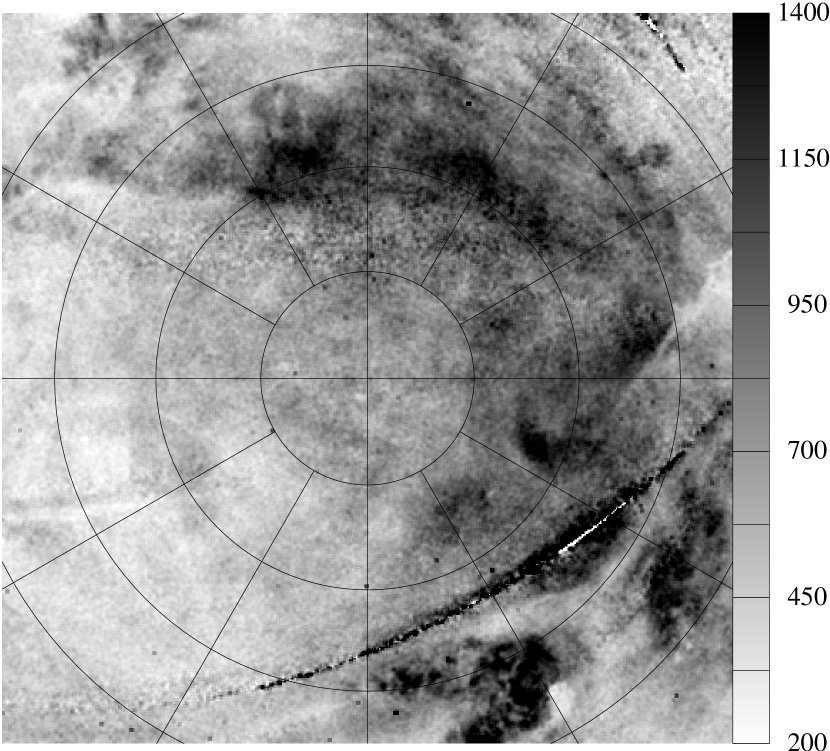
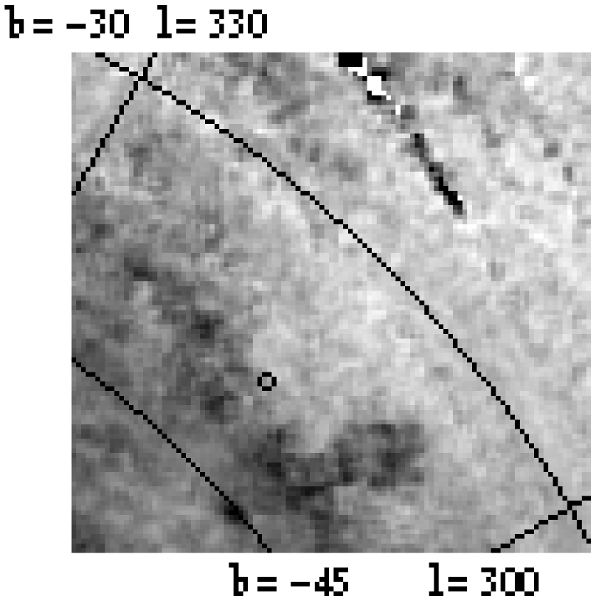
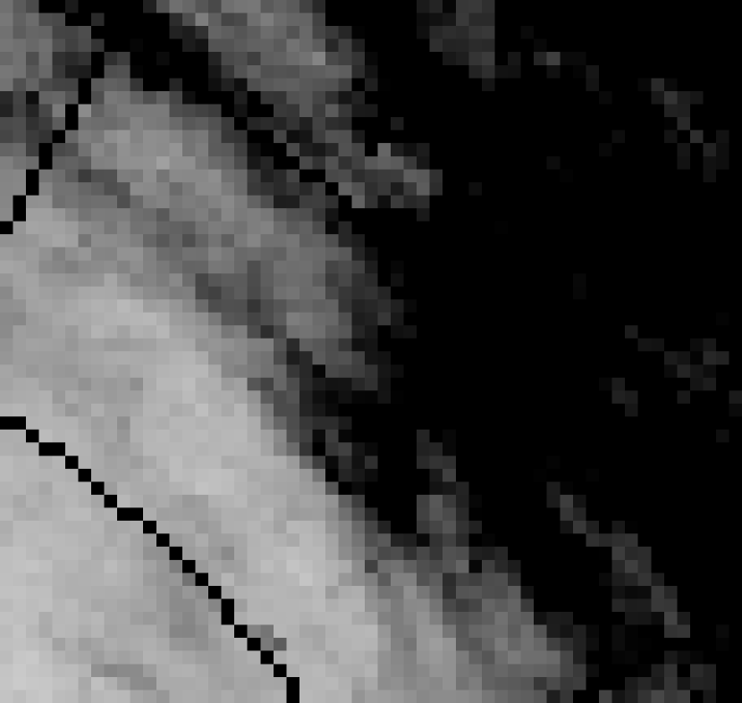
Figure 1: Top: The ROSAT $\frac{1}{4}$ keV surface brightness map of the southern Galactic pole reproduced from Snowden et al. (1997), courtesy of Steve Snowden. The Galactic latitude is $-90^{\rm{o}}$ at the center of the map and increases outward. Lines of latitude are drawn every 15^∘. The Galactic longitude is $0^{\circ}$ at the top of the map. Longitude increases counterclockwise, with meridians drawn every $30^{\circ}$. The units on the sidebar are $10^{-6}$ counts s^-1 arcmin^-2. The dark arc running across the lower right quadrant indicates a region lacking sufficient ROSAT All Sky Survey data. The $\frac{1}{4}$ keV surface brightness for $l=315^{\circ}$, $l=-41^{\circ}$ is approximately average for the region of the southern Galactic hemisphere away from the plane. Bottom Left: Enlargement of the upper right corner of the X-ray map. A circle is drawn around $l=315^{\circ}$, $b=-41^{\circ}$. Bottom Right: DIRBE-corrected IRAS 100 $\mu$m map, reproduced from Snowden et al. 1997.

Soft X-ray data provide some information on the conditions of the hot gas along the observed line of sight, although the plasma producing the soft X-rays is probably somewhat hotter or more highly ionized than the plasma producing the O VI photons. Within a $\sim 5^{\circ}$ radius of the FUSE pointing, the average ROSAT $\frac{1}{4}$ keV surface brightness is $850\times 10^{-6}$ counts s^-1 arcmin^-2 (Kuntz 2000). Figure 1 shows the Snowden et al. (1997) $\frac{1}{4}$ keV map of the sky; the surface brightness at the position of the FUSE pointing is similar to the average observed for latitudes $b<-30^{\circ}$. The map also shows that the pointing direction is not toward an unusual portion of the southern sky. The observed region lies between extended regions of above- and below- average soft X-ray intensities, where the X-ray intensity gradient appears to be associated with absorption by the Galaxy’s H I layer (see Figure 1).

IRAS maps of 100 $\mu$m emission (Wheelock et al. 1994) show that an irregular patch of far-infrared (FIR) cirrus, about 30^′ in diameter, overlaps our 30” $\times$ 30” FUSE field of view. Atomic hydrogen maps (21 cm) yield N${}_{\rm{HI}}\sim$ 4 $\times 10^{20}$ cm^-2, although, due to the coarse binning (Dickey & Lockman 1990; accessed through SkyView at http://skyview.gsfc.nasa.gov/skyview.html), significant variations are possible. Based on published photometry and spectral classification we have also derived estimates of the visual extinction in this region. Using a search radius of 60′, centered on our pointing direction, we find 8 stars with spectral classification in the Michigan Spectroscopic Survey (Houk & Cowley 1975) and B-V measurements from Tycho photometry (Hog et al. 2000). Their spectroscopic and parallax information is listed in Table 1. Using spectroscopic parallaxes we find weak evidence for an obscuring “cloud” at $\sim$200 pc causing a color excess of as much as ${\rm E(B-V)}\sim 0.07$ magnitude, with no evidence for further reddening out to $\sim 750$ pc. This reddening is consistent with the column density derived from the 21 cm data (Diplas & Savage 1994), and we assign it to the FIR (100 $\mu$m) cirrus patch.

Far-ultraviolet emission (e.g., from O VI 1032 and 1038 Å) originating from beyond the cirrus will be subject to scattering and absorption by the cirrus. However, because both the emission source and the cirrus are probably extended, many of the 1032 and 1038 Å photons scattered out of the beam may be replaced by 1032 and 1038 Å photons scattered into the beam. Because we do not know the details of either the source geometry or the FUV scattering characteristics in this direction, we can only estimate the effective amount of extinction experienced by photons originating from beyond the cirrus. In one limiting case, there are losses due to both scattering and absorption, so the average interstellar extinction curve can be applied to estimate the extinction near 1032 and 1038 Å. For E(B-V) $\leq$ 0.07 and R_V=3.1 (the standard value for the diffuse ISM), we find that the extinction curve and parameterization presented in Fitzpatrick (1999) yields A${}_{1035}\leq 0.99$ mag. Transforming this into an optical depth and applying the basic radiative transfer equation, this yields an estimated loss of intensity of $\leq 60\%$. In the other limiting case, all photons scattered out of the beam are replaced by photons scattered into the beam. In this case, there are no net losses due to scattering but there are losses due to absorption. For the cases in which scattering is inconsequential and absorption alone is very small or the sight line traverses a low density section of the cirrus, we take as the extreme lower limit a 0$\%$ loss in intensity. By combining these cases, we take as reasonable limits that between $40\%$ and $100\%$ of the 1032 and 1038 Å intensity that enters the cirrus from beyond will emerge from the cloud and arrive at the observer.

3 Observations and Data Reduction

The observations discussed here were acquired in 1999 September using the low resolution (LWRS; 30″ $\times$ 30″) aperture of the FUSE instrument. Summaries of the FUSE observatory and on-orbit characteristics can be found in Sahnow et al. (2000). The data sets used in this work are archived under the program identification I20509. This paper only presents data taken with detector 1 because detector 2 was off during much of the observations. After eliminating intervals when the spacecraft was in the South Atlantic Anomaly and editing out event bursts (Sahnow et al. 2000), the exposure durations with the 1A and 1B detector segments were 219 and 233 ksec, respectively. Of these, 101 and 99 ksec, respectively, were acquired while the satellite was in the night portion of its orbit. The differences between day and night data are discussed below.

The data were processed using version 1.7 of the standard CALFUSE pipeline (Sahnow et al. 2000; Oegerle, Murphy, & Kriss 2000), with four modifications: (1) the background noise originating in the detector was reduced by excluding counts which produced pulseheights outside the expected range for cosmic photons (the CALFUSE pipeline cutoffs were 4 and 12 in the standard arbitrary units), (2) the standard CALFUSE detector-background subtraction algorithm was not used, allowing us to calculate the uncertainties in our measurements more easily, (3) we extracted the spectra from the spatially corrected two-dimensional images of the detectors’ signal in units of counts reported as an intermediate CALFUSE pipeline data product, and in constructing the extraction windows, we used the the criterion that they must be extended far enough in the cross dispersion direction to at least encompass the entirety of each terrestrial airglow diffuse emission signal, (4) the LiF 1B point source effective area curve, which corrects for the thin shadow of the repeller grid seen in point source spectra over the $\sim 1155$ to $\sim 1170$ Å range (also known as the “worm”), was replaced with an effective area curve that does not include this correction. The relative wavelength scale of the resulting spectrum is accurate to five or six detector pixels, or about 0.035 Å in the LiF 1A spectrum. The absolute wavelength scale is less well known, and we discuss the determination of a wavelength (velocity) zero-point below. The intensity calibration was achieved using the best instrumental affective area estimates as of June 2000 (Sahnow et al. 2000). The uncertainties in the solid angle of the aperture and effective area calibration are the largest sources of systematic error. The LWRS’s solid angle is thought to be accurately known to about $10\%$, while the effective area calibration is thought to be accurate to $\sim 10\%$ for LiF 1A, SiC 1A, and SiC 1B, and $\sim 20\%$ for the LiF 1B outside of the region of the “worm.”

Figure 2 presents the spectra extracted from the detector 1 data in counts versus wavelength (i.e., no intensity calibration has been performed). LiF and SiC refer to the lithium fluoride and silicon carbide mirror and grating coatings used on the respective channels. The strongest emission lines seen in Figure 2 come from the Earth’s atmosphere. Across most of the bandpass, we see only noise due to the detector background, light scattered within the spectrograph, and cosmic background radiation. The small elevations in the intensity between $\sim 1045$ and $\sim 1055$ Å in the LiF 1A spectrum and between $\sim 1025$ and $\sim 1035$ Å in the SiC 1A spectrum are due to light scattered within the spectrograph during the day portion of the orbit. This scattered light makes it untenable to use the day time SiC 1A data for analysis of the O VI emission. The night-only portion of the data provides less than half of the total exposure time. For this reason and because the SiC 1A channel has a smaller effective area at 1032 Å than does the LiF 1A channel, the SiC 1A data are not used in the O VI analysis. However, the night SiC 1B data are used to search for S VI 933 and 944 Å and C III 977 Å emission since the LiF data do not cover these wavelengths. As can be seen in Figure 2, the LiF 1A data show a peak in the vicinity of 1032 A that is potentially an O VI line, and another near 1037-1038 A that potentially contains a C II line and the other O VI line.

We considered the possibility that some of the peaks observed in the 1030 to 1040 Å region of the LiF 1A spectrum could be due to light scattered within the spectrograph. Such scattering would be expected to distribute some light in the cross dispersion direction, as with the $\sim 1045$ to $\sim 1055$ Å contamination, which would be visible outside of the spectral extraction region. However, there is no excess of counts perpendicular to the dispersion direction in this region of the LiF 1A spectrum. Thus, we rule out this type of scattering.

We excluded the possibility that the observed 1032, 1037, and 1038 Å emission lines could have come from the Earth’s atmosphere because of their continued strong emission in the satellite-night portion of the observations. Atmospheric airglow emission (such as the H I Lyman-$\beta$ and O I emission lines at rest wavelengths of 1025.7, 1027.4, 1028.2, 1039.2, 1040.0, 1040.9 Å) are roughly an order of magnitude stronger during the satellite-day portions of the observation than during the satellite-night portions. In contrast, the O VI and C II emission features in our data have constant intensity levels between the satellite-night and satellite-day portions of the observation. Thus, the emission features at 1032, 1037, and 1038 Å are not due to terrestrial airglow (see Figure 3).

We examined the possibility that scattered solar emission lines could have produced the features observed in the LiF 1A data. The Sun’s ultraviolet spectrum has been recorded by the Solar Ultraviolet Measurements of Emitted Radiation (SUMER) instrument aboard the Solar and Heliospheric Observatory (SOHO). The two strongest emission lines common to the SUMER bandpass and the combined FUSE LiF 1A and LiF 1B bandpass are the O VI 1031.9 Å line and the 1175.7 Å member of the C III triplet (Curdt et al. 1997). In the solar spectrum, the C III 1175.7 Å line is 0.86 times as bright as the O VI 1032 Å line. Thus, if the 1032 Å photons observed by FUSE came from the Sun, then FUSE should have also observed 1175.7 Å emission with 86$\%$ the intensity level of the 1032 Å emission. But, the FUSE spectrum contains no emission features within at least 1 Å of 1175.74 Å. For $\lambda=1175.74\pm 0.2$ Å, the intensity recorded by FUSE, and measured with the techniques described below, is 360 $\pm$ 400(random) photons s^-1 cm^-2 sr^-1. This provides upper limits to the possible solar contamination of the LiF 1A spectrum at 1032 and 1038 Å of $420\pm 470$(random) and $210\pm 230$(random) photons s^-1 cm^-2 sr^-1, respectively.

The LiF mirrors are physically situated on the shadowed side of the satellite, while the SiC mirrors are on the sun-illuminated side. This motivated us to search for possible solar contamination in the SiC data. The C III 977 Å emission line observed in the solar spectrum was also found in the day time SiC 1B spectrum but was not found in the night time SiC 1B spectrum. The observed intensity is more than can be explained by terrestrial airglow. Thus, we conclude that the SiC 1 data taken during the day portion of the satellite’s orbit may contain solar contamination, but the data taken at night contains no significant contamination.

4 Spectral Analysis

4.1 O VI Emission

Table 2 presents the measured intensities and uncertainties, $\sigma$, the central velocities, the deduced intrinsic full width at half maximum values, and the implied kinetic temperatures for the two O VI features. The values given in Table 2 were determined as follows. The background continuum was found by fitting a polynomial to the spectrum outside of the H I Ly$\beta$ airglow, O I airglow, and next four strongest emission features (the 1032 Å O VI emission line, the 1038 Å O VI emission line, the 1037 Å C II emission line, and a spurious $\sim$1031 Å feature). The continuum was subtracted from the spectrum. The intensities of the O VI emission features were measured by summing the signal over each line. The statistical (random) $1\sigma$ uncertainty in the number of photons in each feature was calculated as the square root of the sum of the signal and background. The $1\sigma$ systematic uncertainty was calculated by adding in quadrature the $10\%$ uncertainties in the aperture solid angle and flux calibration. The wavelength scale was corrected using an interpolation pinned to the rest wavelengths of the four strongest nearby airglow H I and O I emission lines (Morton 1991, 2001) and the CALFUSE wavelengths at which these features were observed. The corrections applied to the 1032 and 1038 Å emission features were $-0.24$ and $-0.23$ Å, respectively. We then calculated the velocities relative to the geocenter and the Local Standard of Rest (LSR). The wavelength scale is probably accurate to within several detector pixels, or about 10 km s^-1, and the centroid determination is probably accurate to within about 10 km s^-1 as well. The line centroids were found by fitting Gaussian functions to the profiles. The observed widths are greater than the widths of the underlying cosmic spectrum because the FUSE instrument convolves the intrinsic spectrum with the instrumental point spread function and the large slit function. In an analysis of unblended O I and Ar I airglow lines in this and other data sets, we found that the instrumental effects are almost completely responsible for the the shapes and widths of the unblended airglow features (e.g., see the O I feature shown in Figure 4). Thus, we take the nearby 1039 Å O I airglow feature’s profile as the net instrumental function. We convolved this function with Gaussian functions of various widths, then compared the results with the observed O VI profiles in order to determine the intrinsic widths of the O VI emission lines. By equating the line dispersion with a thermal width we were able to calculate an upper limit on the kinetic temperature of the emitting plasma.

The measured intensities of the O VI 1032 and 1038 Å emission features are 2930$\pm$290(random)$\pm$410(systematic) and 1790$\pm$260(random)$\pm$250(systematic) photons cm^-2 s^-1 sr^-1, corresponding to detections at $10\sigma$ and $7\sigma$ levels of significance with respect to the random errors. Henceforth, the $\sigma$ associated with the random errors will be denoted by “(r)” and the $\sigma$ associated with the systematic errors will be denoted with by “(s)”. The velocity profiles of these lines are shown in Figure 4. For comparison, the (unresolved) O I airglow profile is also plotted. The 1032 and 1038 Å features have similar central velocities, observed and intrinsic widths, and the observed velocity profiles have roughly similar shapes. The agreement corroborates our conclusion that the 1032 and 1038 Å features are produced by a single species.

The observed ratio of the intensities in the 1032 Å and 1038 Å lines (calculated from unrounded values; the values in Table 2 were rounded to 3 significant digits) is 1.64$\pm$0.29(r). The systematic uncertainties affect the 1032 and 1038 Å emission line measurements in the same manner and thus the ratio of the 1032 and 1038 Å intensities is not affected by the systematic uncertainties. In the limit of the optically thin case, as the optical depth approaches zero, the ratio should approach that of the statistical weights, 2. In the optically thick case, self absorption may change the ratio. The resulting ratio depends on the optical depth and the geometry of the O VI-rich material. The ratio that we have observed lies 1.2 $\sigma$ below the theoretical optically thin value. The upper limits on the kinetic temperature surpass the temperature at which O VI is most abundant in collisional ionization equilibrium plasma, but the breadths of the O VI profiles could in large part be due to non-thermal processes such as turbulence or dispersion in bulk motions.

4.2 C II Emission

We have also observed emission from the 3s ${}^{2}S_{1/2}$ to 2p ${}^{2}P_{3/2}$ transition of C II ($\lambda=1037.02$ Å). The emission appears to be centered at a corrected LSR wavelength of 1037.16 Å. The emission probably arises from the ${}^{2}S_{1/2}$ to ${}^{2}P_{3/2}$ transition rather than the ${}^{2}S_{1/2}$ to ${}^{2}P_{1/2}$ transition to ground state C II ($\lambda=1036.34$ Å). This is probably because (1) the apparent wavelength is much closer to $1037.02$ Å than to $1036.34$ Å, (2) the A value for the ${}^{2}S_{1/2}$ to ${}^{2}P_{3/2}$ transition is more than twice that of the ${}^{2}S_{1/2}$ to ${}^{2}P_{1/2}$ transition, and (3) the ISM’s plentiful population of ground state C II should readily absorb 1036.34 Å photons.

Table 3 presents the observed intensity, $\sigma$, central LSR velocity, and width of the Gaussian fit to the 1037 Å feature. The emission feature is redshifted relative to rest, but to a slightly lesser degree than the O VI lines. The C II feature is also significantly narrower than the O VI features, as might be expected from gas in a lower ionization stage. The observed FWHM is similar to the instrumental FWHM for diffuse emission that fills the large aperture, i.e., the C II emission line is poorly resolved.

4.3 Search for H₂ Fluorescence between 1031 and 1038 Å:

Hydrogen molecules in high rotational states have several possible transitions that would produce 1032 to 1038 Å photons. We have applied two tests to confirm that the emission lines observed by FUSE are indeed those of the O VI doublet and C II (${}^{2}S_{1/2}$ to ${}^{2}P_{3/2}$) rather than fluorescing H₂. In the first test, we set limits on the strength of the H₂ lines in the vicinity of 1032 Å and 1038 Å by finding other lines in the FUSE bandpass that would be excited by the same mechanism and using the FUSE spectrum to measure their strengths. Morton & Dinerstein (1976), Sternberg (1989), and Abgrall et al. (1993a,b) list the following H₂ emission lines: Lyman (6,0) P(3) transition at 1031.19 Å, Werner (1,1) P(2) transition at 1031.36 Å, Werner (1,1) Q(3) transition at 1031.87 Å, Lyman (6,0) R(4) transition at 1032.35 Å, Lyman (5,0) R(1) transition at 1037.15 Å, and Lyman (5,0) P(1) transition at 1038.16 Å. In order for an H₂ molecule to make the Lyman (6,0) P(3) transition, the ambient radiation field must have first pumped the molecule to the J=2 rotational state, v^′ = 6 vibrational state, and B${}^{1}\sum_{u}$ electronic excitation state. The strength of the Lyman (6,3) P(3) (1172.38 Å) transition arising from the same upper state should be 58% as strong as the Lyman (6,0) P(3) transition at 1031.19 Å(Abgrall et al. 1993a). We have searched the wavelength-corrected FUSE spectrum for emission at this wavelength having the width of the nearest airglow line, finding an integrated intensity of -1300 $\pm$ 620 photons cm^-2 s^-1 sr^-1. Thus, fluorescing H₂ molecules probably are not contributing 1031.19 Å photons. We have applied this method to each of the H₂ transitions above. In every case, the signal is less than 2$\sigma$. We used the Sternberg (1989) model for our second test. In Sternberg’s spectrum of H₂ lines emitted by cool clouds bathed in ultraviolet light, the Q(1) Werner (0,0) line at $\sim 1009.77$ Å and the P(3) Werner (0,1) line at $\sim 1058.82$ Å should be at least 138% and 152% as bright as any of the H₂ emission lines between 1030 and 1040 Å. We have measured the intensities of these comparison lines, finding integrated intensities of 39 $\pm 110$ and 72 $\pm 170$ photons cm^-2 s^-1 sr^-1, respectively. Thus, H₂ fluorescent emission is unlikely to be responsible for the intensities observed near 1032, 1037, and 1038 Å.

4.4 Upper Limits on Other Emission Lines:

We searched the LiF 1A and 1B spectra for interstellar emission from C I at 1122.260 Å, Si II at 1023.700 Å, S III at 1015.502 Å, S IV at 1062.664 Å, and Fe III at 1122.524 Å and we searched the night time SiC 1B spectra for interstellar emission from S VI at 933.378 and 944.523 Å and C III at 977.020 Å. No evidence for emission from any of these lines was found. The resulting 3$\sigma$ upper limits are listed in Table 4.

5 Physical Characteristics

In this section, we derive equations that relate the observed intensities of the O VI emission lines, the optical depths of the emitting regions in these lines, the intrinsic intensities of their emission, and the column densities of the lines. Additional equations relating the intrinsic emission intensity and the column densities to the electron density, thermal pressure and physical extent of the emitting region or regions are also presented. We then calculate the physical characteristics for the following cases of interest. In cases $\#1a$ and $\#1b$, the above quantities are calculated from the observed line intensities and their ratio. In case $\#1a$, we assume that there is no extinction by the possible cirrus material. In case $\#1b$, we assume that the cirrus reduces the 1032 and 1038 Å intensities by $60\%$. The uncertainties in the values calculated for cases $\#1a$ and $\#1b$ are very large, primarily owing to the large uncertainties in the line ratio. Thus we also consider cases $\#2$, $\#3a$, and $\#3b$, which draw the O VI column density from assumptions about the physical scenario rather than the line ratio. In case $\#2$, the sole source of the observed emission is assumed to be the Local Bubble and therefore an estimate appropriate for the Local Bubble is taken for the column density. No cirrus extinction is assumed for case $\#2$ because the cirrus material is thought to lie beyond the Local Bubble. In cases $\#3a$ and $\#3b$, the observed emission is assumed to originate partly in the Local Bubble and partly in the Galactic thick disk and lower halo. Therefore an appropriate estimate is taken for the column density. In case $\#3a$, we assume that there is no extinction by the possible cirrus material. In case $\#3b$, we assume that the cirrus reduces the 1032 and 1038 Å intensities by $60\%$. Cases $\#2$ and $\#3$ are probably the most plausible.

After presenting the results for each of these cases, we discuss five significant assumptions made in this analysis (especially the assumptions of negligible scattering of 1032 and 1038 Å photons into the beam), consider their validity, and discuss the sensitivity of our results to these assumptions. Finally, we use the various derived physical characteristics to constrain the possible sources for the observed emission.

5.1 Derivations

Our first goal is to determine how the observed intensities in the 1032 and 1038 Å lines are related to the intrinsic intensities. By intrinsic intensity, we mean the intensity of photons produced in the plasma. This intensity would have been observed if resonant scattering and extinction by dust had not changed the number of photons heading toward our detector.

By using a self absorption analysis, we are able to link the observed and intrinsic intensities to one another via the optical depth term, and find a ready explanation for the difference between the observed line ratio and the optically thin value. Note, however, that the difference between the observed line ratio and the optically thin value is only marginally statistically significant. In the self absorption scenario, photons emitted by the O VI ions may be scattered out of the beam by interactions with other O VI ions within the emitting region and residing along the line of sight, while only negligible numbers of photons produced by other O VI ions in the emitting region are scattered into the beam. In section 5.3, we question this assumption and discuss how the calculated quantities would be affected if non-negligible numbers of 1032 and 1038 Å photons were scattered into the beam.

The standard radiative transfer equations governing emission produced within a slab of material for the case of negligible scattering into the beam and negligible extinction by dust are Spitzer’s (1978) equations (3-1), (3-2), and (3-3) for the case where no externally produced radiation is incident upon the slab and $j_{\nu}/\kappa_{\nu}$ is constant with respect to $\tau_{\nu}^{\prime}$. These equations yield the observed intensity per frequency interval for a given emission line:

$$I_{o\nu}=\int_{0}^{\tau_{\nu}}\frac{j_{\nu}}{\kappa_{\nu}}e^{-\tau_{\nu}^{\prime}}d\tau_{\nu}^{\prime}=\frac{j_{\nu}}{\kappa_{\nu}}(1-e^{-\tau_{\nu}})$$ (1)

and the intrinsic intensity per frequency interval:

$$I_{i\nu}=\int_{0}^{\tau_{\nu}}\frac{j_{\nu}}{\kappa_{\nu}}d\tau^{\prime}_{\nu}=\frac{j_{\nu}}{\kappa_{\nu}}\tau_{\nu},$$ (2)

where $\nu$ is the frequency, $I_{\nu}$ is the specific intensity per unit frequency, $j_{\nu}$ is the emissivity coefficient, $k_{\nu}$ is the absorption coefficient, $\tau^{\prime}_{\nu}$ is the optical depth variable, and $\tau_{\nu}$ is the total optical depth through the emitting region. Following Spitzer, in our radiative transfer derivations $I_{\nu}$ is in units of ergs cm^-2 s^-1 sr^-1 Hz^-1, $j_{\nu}$ is in units of ergs cm^-3 s^-1 sr^-1 Hz^-1, and $k_{\nu}$ is in units of cm^-1. However, when presenting the results, we give the specific intensity in units of photons cm^-2 s^-1 sr^-1 Hz^-1.

We combine Spitzer’s equations (3-16), (3-23), and (3-25) to yield an expression for $\tau_{\nu}$. The gas is assumed to be far from equivalent thermodynamic equilibrium though it may be in collisional ionizational equilibrium. Thus Spitzer’s $\frac{b_{k}}{b_{j}}$ can be taken as zero, because the populations of the upper levels are negligible. Thus,

$$\tau_{\nu}=N_{j}\frac{\pi e^{2}f_{jk}}{m_{e}c}<\phi(\Delta\nu)>,$$ (3)

where $N_{j}$ is the column density of ions in the $j$ state, $\Delta\nu=\nu-\nu_{o}$, $\nu_{o}$ is the frequency at line center, $<\phi(\Delta\nu)>$ is the line profile function (the path length-averaged normalized distribution with respect to frequency of the cross section per O VI ion), $e$ is the charge of the electron, $f_{jk}$ is the oscillator strength for the chosen transition, $m_{e}$ is the mass of the electron, and $c$ is the speed of light. From Spitzer’s equation (3-25), $\frac{\pi e^{2}}{m_{e}c}=2.654\times 10^{-2}$, where the units should be $\frac{\rm{cm}^{2}}{\rm{s}}$. If the particle velocity distribution is Maxwellian, then $<\phi(\Delta\nu)>=\frac{\lambda}{b\sqrt{\pi}}e^{-(\frac{\lambda\Delta\nu}{b})^{2}}$. Here $b$ is the velocity-spread parameter, $\Gamma_{v}$ is the FWHM velocity, and $b=0.6\Gamma_{v}$. If we define $\tau_{o}$ as the optical depth at line center, then

$$\tau_{\nu}=N_{j}\frac{\sqrt{\pi}e^{2}f_{jk}\lambda}{m_{e}cb}e^{-(\frac{\lambda\Delta\nu}{b})^{2}}=\tau_{o}e^{-(\frac{\lambda\Delta\nu}{b})^{2}}.$$ (4)

We now integrate equations (1) and (2) with respect to $\nu$ in order to determine $I_{o}$ and $I_{i}$. Assuming that $j_{\nu}/\kappa_{\nu}$ is constant over the frequency interval where $1-e^{-\tau_{\nu}}$ differs from $0$,

$$I_{o}=\frac{j_{\nu_{o}}}{\kappa_{\nu_{o}}}\int_{0}^{\infty}(1-e^{-\tau_{\nu}})d\nu=\frac{2j_{\nu_{o}}}{\kappa_{\nu_{o}}}\int_{0}^{\infty}(1-e^{-\tau_{o}e^{-(\frac{\lambda\Delta\nu}{b})^{2}}})d(\Delta\nu).$$ (5)

Equation (4) of Jenkins (1996) provides a solution to the integral in our equation (5) for $\tau_{o}\stackrel{{\scriptstyle<}}{{\sim}}15$: $F(\tau_{o})=\int_{0}^{\infty}[1-e^{(-\tau_{o}e^{-x^{2}})}]dx=\frac{\sqrt{\pi}}{2}\sum_{n=1}^{\infty}\frac{(-1)^{n-1}\tau_{o}^{n}}{n!\sqrt{n}}$. For $x=\frac{\lambda\Delta\nu}{b}$, we find

$$I_{o}=\frac{\sqrt{\pi}b}{\lambda}\frac{j_{\nu_{o}}}{\kappa_{\nu_{o}}}\sum_{n=1}^{\infty}\frac{(-1)^{n-1}\tau_{o}^{n}}{n!\sqrt{n}}=\frac{2b}{\lambda}\frac{j_{\nu_{o}}}{\kappa_{\nu_{o}}}F(\tau_{o}).$$ (6)

If there is dust between the emitting plasma and the observer, then equation (6) must be modified to account for the losses due to extinction. Equation (6) becomes:

$$I_{o}=\frac{a2b}{\lambda}\frac{j_{\nu_{o}}}{\kappa_{\nu_{o}}}F(\tau_{o}),$$ (7)

where $a$ is the ratio of the intensity that emerges at the near side of the dust to the intensity that impinges upon the far side of the dust. As discussed in section 2, if the O VI-rich gas is beyond the IRAS cirrus patch, then $a$ is likely between 0.4 and 1.0.

Assuming that $j_{\nu}/\kappa_{\nu}$ is approximately constant over the range of $\nu$ where $\tau_{\nu}\neq 0$, the integrated intrinsic intensity is:

$$I_{i}=\frac{j_{\nu_{o}}}{\kappa_{\nu_{o}}}\int_{0}^{\infty}\tau_{\nu}d\nu=\frac{2j_{\nu_{o}}}{\kappa_{\nu_{o}}}\int_{0}^{\infty}\tau_{o}e^{-(\frac{\lambda\Delta\nu}{b})^{2}}d(\Delta\nu)=\tau_{o}\frac{\sqrt{\pi}b}{\lambda}\frac{j_{\nu_{o}}}{\kappa_{\nu_{o}}}.$$ (8)

We will use the ratio of equation (7) to equation (8) to calculate the intrinsic intensities from the observed intensities. This requires knowing the optical depth for each emission line: $\tau_{o(1032)}$ and $\tau_{o(1038)}$. If the column density is known, then equation (4) can be used to determine each $\tau_{o}$. Otherwise, the optical depths can be estimated from the ratio of the observed intensities in the 1032 and 1038 Å lines in the following manner. The oscillator strength for the 1032 Å transition is twice that for the 1038 Å transition and the ratio of $j_{\nu}/\kappa_{\nu}$ is given by Spitzer’s equation (3-31), thus, $\tau_{o(1032)}$ is equal to $2\tau_{o(1038)}$ and $\frac{j_{\nu_{o}(1032)}}{\lambda_{(1032)}\kappa_{\nu_{o}(1032)}}/\frac{j_{\nu_{o}(1038)}}{\lambda_{(1038)}\kappa_{\nu_{o}(1038)}}$ is equal to $(\frac{\lambda_{(1038)}}{\lambda_{(1032)}})^{4}$. The resulting ratio of equation (7) for the 1032 Å line to equation (7) for the 1038 Å line is:

$$\frac{I_{{o(1032)}}}{I_{{o(1038)}}}=\frac{\lambda_{(1038)}^{4}F(2\tau_{o(1038)})}{\lambda_{(1032)}^{4}F(\tau_{o(1038)})}.$$ (9)

This can be solved for $\tau_{o(1038)}$.

Next we determine the average electron density from the intrinsic intensity and the column density. The following equation motivated our earlier derivations of the intrinsic intensity and column density. Shull & Slavin (1994) present a relation for the average electron density of an emitting region in which the kinetic temperature and emissivity per O VI ion are constant:

$$\langle n_{e}\rangle=\frac{4\pi}{\langle\sigma v\rangle_{e}}\;\frac{(I_{i5000})}{N_{OVI}}=$$ (10)

$$(0.00921\;{\rm cm}^{-3})\;\Biggl{[}\frac{5}{\bar{\Omega}_{OVI}(T)}\Biggr{]}\;T_{5}^{1/2}\;\exp\;\biggl{(}\frac{1.392}{T_{5}}\biggr{)}\;\frac{I_{i5000}}{N_{14}},$$

where $\langle\sigma v\rangle_{e}$ is the electron-impact excitation-rate coefficient for the 1032 and 1038 Å lines combined, $\bar{\Omega}_{OVI}(T)$ the Maxwellian-averaged collision strength for de-excitation of the O VI doublet, $T$ is the gas temperature, $T_{5}$ the gas temperature in $10^{5}$ K, $N_{14}$ the column density in units of $10^{14}$ cm^-2, and $I_{i5000}$ the intrinsic O VI doublet intensity in units of 5000 photons cm^-2 s^-1 sr^-1. Shull & Slavin present a parameterization of the Maxwellian-averaged collision strength: $\bar{\Omega}_{OVI}(T)=6.43[0.5584+(0.1363y-0.1158y^{2}+0.279)E_{1}(y)e^{y}+0.1158y]$, where $y=E_{o}/kT$ and $E_{1}(y)$ is the first exponential integral, $\int_{y}^{\infty}\frac{e^{-x}}{x}dx$.

The thermal pressure can also be calculated. Assuming a cosmic abundance of helium and complete ionization of both hydrogen and helium,

$$P_{th}/k=1.92n_{e}T.$$ (11)

We expect the relevant temperatures to be near $3.2\times 10^{5}$ K because this is the temperature at which the fraction of oxygen atoms in the O VI ionization state is greatest (Shapiro & Moore 1976). The O VI ions could exist within plasmas of a range of temperatures. For example, the fraction of oxygen atoms in the O VI ionization state is at least 10$\%$ of its maximum value in collisional ionizational equilibrium plasmas for temperatures between $2.2$ and $6.4\times 10^{5}$ K. The electron density calculated from equation (10) varies little across this range.

The depth of the emitting region ($\Delta l$ or $\int dl$) is related to the column density through $N_{OVI}=\int n_{OVI}dl$, where $n_{OVI}$ is the density of O VI ions. Thus, $\Delta l$ is approximately equal to $N_{OVI}/n_{OVI}$. The volume density of O VI ions can be found from $n_{OVI}=n_{e}\times\frac{n_{H}}{n_{e}}\times\frac{n_{O}}{n_{H}}\times\frac{n_{OVI}}{n_{O}}$, where $n_{e}$, $n_{H}$, and $n_{O}$ are the densities of electrons, hydrogen atoms, and oxygen atoms respectively. For a cosmic abundance of helium and complete ionization of both hydrogen and helium, $n_{e}$ is equal to $1.2n_{H}$. Using the Grevesse and Anders (1989) solar abundance of oxygen, $n_{O}$ is equal to $8.5\times 10^{-4}n_{H}$. According to the Shapiro and Moore (1976) collisional ionizational equilibrium curve for oxygen, the maximum value of $n_{OVI}/n_{O}$ is 0.26. This occurs at $T=3.2\times 10^{5}$ K. The resulting equation for $\Delta l$ is,

$$\Delta l=5400\times\frac{N_{OVI}}{n_{e}},$$ (12)

where $T$ is assumed to be $3.2\times 10^{5}$ K, $N_{OVI}$ is in cm^-2, $n_{e}$ is in cm^-3, and $\Delta l$ is in cm. Although most of the O VI ions probably reside within gas having nearly the maximum value of $n_{OVI}/n_{O}$, some of the ions may reside in hotter or cooler gas.

5.2 Calculated Values for the Physical Characteristics

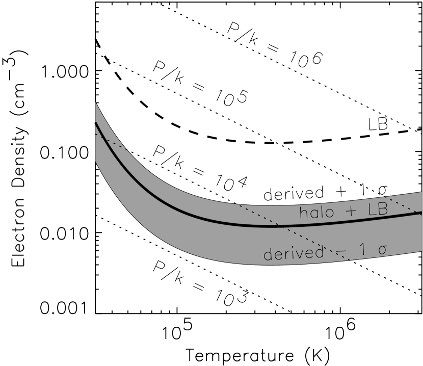
Figure 5: The electron density $n_{e}$ as a function of temperature for an O VI plasma, assuming values calculated directly from the data (case $\#1a$, shaded region), values calculated from the data and an assumed O VI Local Bubble column density (case $\#2$, dashed line), and values calculated from the data and an assumed Local Bubble plus thick disk and lower halo column density (case $\#3a$, thick solid line). Overplotted are lines of constant thermal pressure ($P_{th}/k=1.92n_{e}T$, dotted lines).

In this subsection, we use equations (4), (7), (8), (9), (10), (11), and (12) to relate the observed intensities, optical depths, intrinsic intensities, column densities, electron densities, thermal pressures, and approximate emitting depth. The results are presented in Table 5 and Figure 5. In case $\#1a$, we take $a=1.0$ and use the observed intensities and equation (9) to determine $\tau_{o(1038)}$, finding $\tau_{o(1038)}=0.79_{-0.61{\rm{(r)}}}^{+1.38{\rm{(r)}}}$. There is no systematic uncertainty in $\tau_{o}$ calculated from the ratio of the observed intensities. Then $\tau_{o(1032)}$ is calculated from $\tau_{o(1038)}$. We use the optical depths, observed intensities, and the ratio of equation (8) to equation (7) to calculate the intrinsic intensities for the emission lines. The resulting intrinsic intensity of the doublet is $7,100^{+19,100{\rm{(r)}}}_{-2,900{\rm{(r)}}}\pm 1000{\rm{(s)}}$ photons s^-1 cm^-2 sr^-1. We calculate the velocity parameter from the velocity FWHM in Table 2. We use the velocity parameter and $\tau_{o}$ to calculate the column density in the ground state, finding $N=5.1_{-3.9{\rm{(r)}}}^{+8.9{\rm{(r)}}}\times 10^{14}$. Note that due to the uncertainty in the observed line ratio, the uncertainty in $N$ is very large. We use the doublet intensity, column density, and equation (10) to calculate the electron density for $T=3.2\times 10^{5}$ K, yielding $n_{e}=0.0060^{+0.016{\rm{(r)}}}_{-0.0024{\rm{(r)}}}\pm 0.0008{\rm{(s)}}$. As equation (10) and Figure 5 show, the electron density varies little between $T=2\times 10^{5}$ and $2\times 10^{6}$ K. We use equation (11) to calculate the thermal pressure at this temperature, finding $P_{th}/k=3,700^{+9,900{\rm{(r)}}}_{-1,500{\rm{(r)}}}\pm 520{\rm{(s)}}$. Equation (12) is used to calculate the emitting depth if the gas is at this temperature, finding $\Delta l=4.6^{+15{\rm{(r)}}}_{-4.0{\rm{(r)}}}\pm{0.64}{\rm{(s)}}\times 10^{20}$ cm, or $150^{+480{\rm{(r)}}}_{-130{\rm{(r)}}}\pm{21}{\rm{(s)}}$ pc.

This process is repeated for $a=0.4$ in case $\#1b$. Table 5 presents the results for each case. In the table, $\Delta l$ is presented in units of parsecs. The calculated uncertainties are rather large for some of the tabulated characteristics. The main source of the propagated uncertainties in cases $\#1b$ and $\#1b$ is the relatively large uncertainty in the line ratio. As a result, it is instructive to examine cases in which the column density (and hence the ratio of observed intensities) is set by the assumption of a particular geometry. In case $\#2$, the emission is assumed to originate in the Local Bubble. For this case we take the absorption column density to be $N_{OVI}\approx 1.6\times 10^{13}$ cm^-2 (Shelton & Cox 1994). Only negligible extinction is expected, so $a$ is taken to be 1.0. From the column density, we determine the optical depths and the ratio of intensities observed in the 1032 Å and 1038 Å emission lines. The total observed intensity is assumed to be conserved. We then calculate the other quantities using the same method as in cases $\#1a$ and $\#1b$. The results are presented in Table 5 and Figure 5.

In cases $\#3a$ and $\#3b$, the observed emission is assumed to originate in part in the Local Bubble and in part the Galactic thick disk and lower halo. For these cases, we take the absorbing column density to be $N_{OVI}=2.0\times 10^{14}$ cm^-2 from Savage et al. (2000). Because the previously discussed cirrus may lie either closer than the thick disk/halo emission region or beyond it, the physical characteristics are calculated using $a=1.0$ (case $\#3a$) and $a=0.4$ (case $\#3b$). The calculations follow the same method as in case $\#2$ and are presented in Table 5 and Figure 5. Note that in this model, the Local Bubble, thick disk, and lower halo are assumed to have the same thermal pressure. This is the pressure calculated from the equations and listed in Table 5.

5.3 Caveats

In this analysis, we have made the following assumptions, which we will discuss in more detail in the remainder of this section. 1.) The contribution of 1032 and 1038 Å photons emitted by other O VI ions in the “cloud” but outside of the beam and scattered into the beam via interactions with O VI ions is assumed to be negligible when compared with the number of such photons scattered out of the beam via such interactions. 2.) The contribution due to scattering of background ultraviolet continuum photons is assumed to be negligible. 3.) Losses due to other types of particles interspersed with the O VI ions are assumed to be negligible (though the calculations do consider an external region of extincting particles). 4.) The emissivity per O VI ion is assumed to be constant. 5.) Furthermore, by using equations (10) and (11), we make the assumption that the temperature and $n_{OVI}/n_{O}$ ratio are near their values at the peak of the ion fraction curve constructed by Shapiro and Moore using collisional ionization equilibrium.

If the first assumption is not valid then the intrinsic doublet intensities will be less than the calculated values. The degree of scattering into the beam is not known. If the number of photons produced by the O VI “cloud” and scattered into the beam via interactions with O VI ions compensates exactly for the number produced by the O VI “cloud” and scattered out via interactions with O VI ions, then the intrinsic intensities would not follow equation (7), but would be equal to the observed intensities after correction for dust extinction. The results of such a scenario are within the error bars on our calculated doublet intensities in each of our cases (i.e. $\#1a$, $\#1b$, $\#2$, $\#3a$, and $\#3b$). If the number of photons produced by the O VI “cloud” and scattered into the beam due to interactions with O VI ions were to be even larger than the number produced by the O VI “cloud” and scattered out, then the true intrinsic intensity would be less than the observed intensity after correction for dust extinction. In this scenario, we would expect the 1032 Å intensity to be at least twice as strong as the 1038 Å intensity because O VI ions scatter 1032 Å photons more readily. Such a scenario is marginally excluded because the observed ratio of the 1032 and 1038 Å intensities ($1.64\pm 0.29(r)$) is at least 1.24 sigma from the theoretical value ($>$2). In cases $\#1a$ and $\#1b$, if some of the photons scattered out of the beam have been compensated for by photons scattered into the beam, then the true optical depths and column density would be greater than the calculated values. For cases $\#2$, $\#3a$, and $\#3b$, the column densities were assumed and the optical depths were found from them. If some of the light scattered out of the beam were replaced by light scattered into the beam, then the ratio of the observed to the intrinsic intensity would be less than that calculated from equations (7) and (8) using the $\tau_{o}$ calculated from the assumed column density. In all cases, if the intensity scattered into the beam is not negligible when compared with the intensity scattered out of the beam, then the true electron density and thermal pressure would be less than the calculated values.

It is difficult to evaluate the second assumption, primarily because the geometric relationship between the stellar continuum sources and O VI ions is not well known. The following is an order of magnitude estimate. We assume that the O VI ions on the line of sight are bathed in the incident ultraviolet continuum field, whose strength is: $I_{sci}=4.38\times 10^{-20}$ ergs s^-1 cm^-2 sr^-1 Hz^-1 (Mathis, Mezger, & Panagia 1983). The volumetric intensity absorbed by the O VI photons will be $I_{a\nu}=I_{sci}n_{o}\frac{\pi e^{2}f}{m_{e}c}\frac{\lambda}{b\sqrt{\pi}}e^{-(\lambda\Delta\nu/b)^{2}}$. The ions will quickly re-emit this volumetric intensity, but a fraction of the re-radiated photons will arrive at the observer while other photons will be scattered out of the beam due to absorption by intervening O VI ions or will be absorbed by other intervening particles. The observed intensity ($I_{sco}$) can be found by solving Spitzer’s equation (3-1) or our equation (1), where $I_{a\nu}$ is substituted for $j_{\nu}$ and where an extinction factor, $a$, is included. The result is

$$I_{sco}=\frac{a2b}{\lambda}{I_{sci}}F(\tau_{o}).$$ (13)

We use equation (13) to create rough estimates of the possible contribution of scattered ultraviolet continuum photons to the observed intensity. The results are presented in the last column of Table 5. The systematic uncertainties in $I_{sco}$ are bound to be large. As a result, we are not prepared to make confident corrections to the observed O VI intensities at this time. However, it is logical to recognize that if some scattered ultraviolet continuum photons are being observed, then the true intrinsic intensity, electron density, thermal pressure, and emitting depth are less than the values presented in Table 5. In particular, if the estimated scattering is used, then the doublet intensities, electron densities, and thermal pressures in the most plausible cases, cases $\#2$ and $\#3b$, would decrease from the quoted values by $4.0\%$ and $17\%$, respectively. The emission depths would increase by $4.0\%$ and $20\%$, respectively.

In the third assumption, there are no other absorbing particles interspersed with the O VI ions. If this assumption is false and if the calculated extinction by the cirrus is not an overestimate, then the effective extinction would be greater than assumed. Thus, the intrinsic intensities, electron density, and thermal pressure would be greater than the calculated values. The emitting region would be smaller than the calculated value.

In the fourth assumption, the emissivity per O VI ion is assumed to be constant. In case $\#3$ where some of the emission is from the Local Bubble and some is from the halo, the thermal pressure varies along the path length. Thus the electron density and emissivity vary along the path length. The higher pressure gas in the Local Bubble would be more emissive per ion than the lower pressure gas in the thick disk and halo. As a result, in case $\#3$, the pressure listed in Table 5 would lie between the pressure of the gas in the Local Bubble and the pressure of the gas in the thick disk and halo. This logic also applies to case $\#1$.

If the assumptions regarding the temperature and ionization state of the gas are invalid, then the electron density, thermal pressure, and emitting depth are affected. If the gas is near the specified temperatures but out of collisional ionizational equilibrium, then the emitting depths would be larger than calculated from equation (12). Alternatively, if the fraction of oxygen ions in the O VI stage is near the peak in the Shapiro and Moore curve, but the gas temperature is much lower (or somewhat higher) than assumed, then the emissivity would be lower (or higher) than assumed and so the calculated electron density would be higher (or lower) than assumed.

5.4 Possible Locations of the Emitting Gas

In this subsection, we critique possible emission sources. We first examine the possibility that the observed emission originates entirely in the Local Bubble. ROSAT observations of soft X-ray emission from the Local Bubble suggest that the thermal pressure is $\sim 15,000$ K cm^-3 (Snowden et al. 1998). This value was found by fitting the soft X-ray spectrum with model spectra for solar abundance, collisional ionization equilibrium plasma and is appropriate for the $\sim 10^{6}$ K, X-ray emitting plasma. Cool clouds within the Local Bubble have been shown to have lower thermal pressures (i.e. Jenkins (1998)). We assume that the difference between the thermal pressures of the hot and cool gas is balanced by other forms of pressure, such as magnetic or turbulent pressure. Hence, the thermal pressure in the cool gas does not constrain our analysis. The pressure of the soft X-ray emitting gas is within the range of pressures found for case $\#2$.

If we assume that the O VI-bearing gas is in pressure balance with the X-ray emitting gas and that the O VI ions predominately exist within gas of temperatures between 2.2 and $6.4\times 10^{5}{\rm{K}}$, then the electron density is about $\frac{15,000}{1.92\times(2.2{\rm{\ to\ }}6.4\times 10^{5}{\rm{K}})}=0.012$ to $0.036$ cm^-3. Using equation (10) with these temperatures and electron densities and the Shelton & Cox (1994) value for the Local Bubble column yields an intrinsic doublet intensity between $\sim 440$ and $\sim 1300$ photons cm^-2 s^-1 sr^-1. Not only is this range substantially lower than the intrinsic doublet intensity calculated for case $\#2$, it is well below the observed doublet intensity! Scattered ultraviolet continuum photons probably cannot account for the intensity discrepancy because the relatively small Local Bubble O VI column density is ineffective at scattering the assumed incident photon field. Thus, we conclude that the Local Bubble, which is assumed to be in pressure balance and collisional ionizational equilibrium, cannot account for the bulk of the observed O VI  photons. An additional source is needed.

The photons which do originate in the Local Bubble probably come from a thin zone of hot gas. Using a Local Bubble pressure of 15,000 K cm^-3 and equations (10), (11) and (12), we calculate the thickness of the O VI-bearing gas as a function of temperature. If the temperature is $T=3.2\times 10^{5}$ K, then the fraction of oxygen atoms in the O VI ionizational state is at its maximum and $\Delta l=1.1$ pc. If the temperature is $T=2.4\times 10^{5}$ K or $T=6.4\times 10^{5}$ K, where the abundance of O VI ions is $10\%$ of its maximum value, $\Delta l=7.9$ pc or 23 pc, respectively. Thus it is possible that the O VI ions reside in a thin shell on the edge of the Local Bubble. Such a structure is consistent with the lack of O VI column density towards stars located within the interior of the bubble (Oegerle et al. 2001).

If observed emission originates in the Local Bubble, thick disk, and halo, then the derived pressure should be between the thermal pressures of the hot gases in these regions. As mentioned above, the thermal pressure of the hot gas in the Local Bubble is thought to be about $\sim 15,000$ K cm^-3. The thermal pressure in the thick disk and halo ranges from $\sim 0$ at large distances from the Galactic midplane to $\sim 13,000$ K cm^-3 within 2 kpc of the plane in regions where the total pressure is predominately in the form of thermal pressure (Boulares & Cox 1990). The derived pressures for cases $\#3a$ and $\#3b$ are within the allowed range.

From Table 5, depending on dust extinction, the thickness of the emission zone would be 12 to 29 pc if $T=3.2\times 10^{5}$ K. If the temperature is between $2.4$ and $6.4\times 10^{5}$ K, then the values would be larger by a factor of up to 7 and 20, respectively. On a Galactic scale, these values are not large. It is possible that the O VI in the thick disk and lower halo resides in midscale structures scattered about the thick disk and lower halo. Such a scenario would be consistent with the large scale height (2.7 kpc) and high degree of inhomogeneity found in the Savage et al. (2000) mini-survey.

We now examine the expected velocity for the pointing direction. In general, the velocities of the highly-ionized material in this part of the sky can be understood by assuming that a thickened disk of highly-ionized material roughly corotates with the underlying thin disk of low-ionization gas (e.g., Lu et al. 1994; Sembach & Savage 1992). Our measured O VI velocities differ from the velocities expected from co-rotating gas within 10 kpc of the plane by over $100$ km sec^-1. This discrepancy does not rule out the possibility that most of the emitting material resides within the thick disk $/$ halo. It is quite plausible that the O VI resides within shock-heated gas traveling over $100$ km sec^-1 relative to the speed expected from galactic rotation.

A third hypothetical location for the observed material is high- or intermediate-velocity clouds and their environments, but this hypothesis appears to be contradicted by the 21 cm observations. Wakker et al. (2001) have presented Parkes H I 21 cm observations in the direction of the star HD 3175, which lies $\sim 14^{\circ}$ from the FUSE pointing, showing an H I intermediate-velocity cloud at $v_{\rm LSR}\approx+73$ km s^-1 with $N(\mbox{H I})\approx 10^{19}$ cm^-2. However, the H I spectra from the southern H I 21 cm emission survey of the Instituto Argentino de Radioastronomía (Arnal et al. 2000; see also Morras et al. 2000) show no evidence for an H I intermediate-velocity cloud over the velocity range $v_{\rm LSR}\approx+50$ to $+90$ km s^-1 within $\sim 1\fdg 5$ of of the FUSE pointing (R. Morras 2000, private communication).

6 Summary

We have observed emission by O VI ions in the Galaxy’s general diffuse ISM outside of supernova remnants or superbubbles. We have ruled out the possibilities that the observed photons are stellar, instrumental or terrestrial airglow. The observed intensities, velocities, and intrinsic widths are presented in Table 2. We have used the observed properties to estimate the column density, intrinsic intensity, average electron density, thermal pressure, and depth of the emitting gas. The results are presented in Table 5.

The doublet intensity is larger than expected for emission by the (assumed quiescent) Local Bubble alone. Thus, we surmise that some of the observed intensity must arise in the Galactic thick disk or lower halo. There are no H I clouds in the southern H I 21 cm emission survey of the Instituto Argentino de Radioastronomía near this direction at similar velocities. Thus, high velocity clouds are probably not the source of the observed emission. The emitting material appears to be confined to relatively shallow regions such as the edge of the Local Bubble or 10 to 600 pc thick structures in the Galactic halo.

Figure 2: The counts spectra from the $l=315^{\circ}$, $b=-41.3^{\circ}$ pointing. Each spectrum is logorithmically scaled in counts, includes satellite day and night data, and is binned by 11 pixels ($\sim 0.075$ Å for the LiF 1A). The strong, narrow peaks are terrestrial airglow emission lines. The elevations in the LiF 1A count rate at short wavelengths and the SiC 1A countrate at long wavelengths are due to elevated scattered light levels. The small elevations in the intensity between $\sim$1045 and $\sim$1055 Å in the LiF 1A spectrum and between $\sim$1025 and $\sim$1035 Å in the SiC 1A spectrum are due to a localized band of scattered light cutting across the spectrum.

Figure 3: The LiF 1A spectrum, binned over 11 pixels (corresponding to 0.075 Å or about one fifth of the width of the large aperture) and plotted relative to the uncorrected CALFUSE wavelengths. Top: spectrum from the satellite night portion of the data. Middle: spectrum from the satellite day portion of the data. Bottom: spectrum from the day and night data. The emission lines associated with the Earth’s atmosphere (each denoted by $\oplus$) are quite strong in the total and day-only spectra, but much weaker in the night-only spectra. The $\sim$1032 and $\sim$1038 Å emission features of interstellar O VI have similar brightnesses in the night-only and the day-only spectra. The 1037 Å feature of interstellar C II is also present in all spectra. The 1031 Å feature appearing in the total and day-only spectra is absent in the night-only spectra and is not statistically significant in the day-only data, thus is probably not cosmic.

Figure 4: The 1032 and 1038 Å O VI and 1039 Å O I profiles versus LSR velocity and binned by 5 detector pixels. Top: The intensity in the O VI 1032 Å emission feature. For plotting purposes, the curve has been shifted upwards by 65 photons s^-1 cm^-2 sr^-1 (km s^-1)^-1. Middle: Intensity in the O VI 1038 Å feature, shifted upwards by 30 photons s^-1 cm^-2 sr^-1 (km s^-1)^-1. The 1032 Å and 1038 Å features have similar central velocities, widths, and roughly similar envelopes. Bottom: To illustrate that the instrument optics convolve the intrinsic profile with a top hat function, the observed airglow O I 1039 Å profile, scaled by 0.3 and shifted to the right by 65 km s^-1, is also shown.

Table 1: Stars within 60 arcmin of $l=315.0^{\circ}$, $b=-41.3^{\circ}$

Star	Ang. Sep.	Sp. Class	Phot. Dist.	Par. Dist.	E(B-V)
	(arcmin)		(pc)	(pc)
HD214691	37.0	G5V	40	49$\stackrel{{\scriptstyle+2}}{{{}_{-2}}}$	0.05
HD213591	51.0	G0V	53	47$\stackrel{{\scriptstyle+2}}{{{}_{-2}}}$	-0.02
HD213928	53.0	F7/F8V	65	77$\stackrel{{\scriptstyle+5}}{{{}_{-5}}}$	0.01
HD214778	40.0	G2V	97	249$\stackrel{{\scriptstyle+119}}{{{}_{-61}}}$	-0.05
HD214522	59.0	F8/G0V	134		-0.02
HD213742	41.0	K1III	167	175$\stackrel{{\scriptstyle+22}}{{{}_{-17}}}$	0.07
HD216379	58.0	K2III	381	353$\stackrel{{\scriptstyle+190}}{{{}_{-92}}}$	0.07
HD215970	39.0	G8/K0III	741		0.02

Table 2: O VI Observations

Characteristic	O VI  1032 Å feature	O VI  1038 Å feature
Intensity (photons s-1 cm-2 sr-1)	2930	1790
Intensity (photons s-1 cm-2 sr-1)	2930	1790
$\sigma$ due to random uncertainties (photons s-1 cm-2 sr-1)	290	260
$\sigma$ due to systematic uncertainties (photons s-1 cm-2 sr-1)	410	250
Center LSR Velocity (km s-1)	$+70$	$+60$
Intrinsic FWHM (km s-1)	$\sim 110$	$\sim 110$
Kinetic Temperature (K)	$\lesssim 4\times 10^{6}$	$\lesssim 4\times 10^{6}$

Table 3: Characteristics of the C II Emission Feature

Characteristic	C II 1037 Å feature
Intensity (photons s-1 cm-2 sr-1)	1990
$\sigma$ due to random uncertainties (photons s-1 cm-2 sr-1)	260
$\sigma$ due to systematic uncertainties (photons s-1 cm-2 sr-1)	280
Center LSR Velocity (km s-1)	$+$40

Table 4: 3$\sigma$ Upper Limits for Other Transitions

Species	Rest Wavelength	3$\sigma$ Upper Limita
	(Å)	(photons s-1 cm-2 sr-1)
S VI	933.378	3600
S VI	944.523	3600
C III	977.020	2600
S III	1015.502	780
Si II	1023.700	390
S IV	1062.664	350
C I	1122.260	580
Fe III	1122.524	580

Note – $a$:   As described in the text, these measurements are also subject to the systematic uncertianties of $14\%$.