Probing the Intergalactic Medium with the Ly$\alpha$ forest along multiple lines of sight to distant QSOs

Abstract

We present an effective implementation of analytical calculations of the Ly$\alpha$ opacity distribution of the Intergalactic Medium (IGM) along multiple lines of sight (LOS) to distant quasars in a cosmological setting. The method assumes that the distribution of neutral hydrogen follows that of an underlying dark matter density field and that the density distribution is a (local) lognormal distribution. It fully accounts for the expected correlations between LOS and the cosmic variance in the large-scale modes of the dark matter distribution. Strong correlations extending up to $\sim 300$ kpc (proper) and more are found at redshift $z\sim 2\to 3$, in agreement with observations. These correlations are investigated using the cross-correlation coefficient and the cross-power spectrum of the flux distribution along different LOS and by identifying coincident absorption features as fitted with a Voigt profile fitting routine. The cross-correlation coefficient between the LOS can be used to constrain the shape-parameter $\Gamma$ of the power spectrum if the temperature and the temperature density relation of the IGM can be determined indepedently. We also propose a new technique to recover the 3D linear dark matter power spectrum by integrating over 1D flux cross-spectra which is complementary to the usual ‘differentiation’ of 1D auto-spectra. The cross-power spectrum suffers much less from errors uncorrelated in different LOS, like those introduced by continuum fitting. Investigations of the flux correlations in adjacent LOS should thus allow to extend studies of the dark matter power spectrum with the Ly$\alpha$ forest to significantly larger scales than is possible with flux auto-power spectra. 30 pairs with separation of 1-2 arcmin should be sufficient to determine the 1D cross-spectrum at scales of $60\,h^{-1}$ Mpc with an accuracy of about 30% (corresponding to a 15% error of the rms density fluctuation amplitude) if the error is dominated by cosmic variance.

1 Introduction

The current understanding of QSO spectra blueward of Ly$\alpha$ emission, the so-called Ly$\alpha$ forest, is based on the idea that the Ly$\alpha$ absorption is produced by the inhomogenous distribution of the Intergalactic Medium (IGM) along the line of sight (Bahcall & Salpeter 1965; Gunn & Peterson 1965). The IGM is thereby believed to be warm ($\sim 10^{4}$ K) and photoionized. The rather high flux of the ultraviolet background radiation results in a small neutral hydrogen fraction with Ly$\alpha$ optical depth of order unity which is responsible for a ‘fluctuating Gunn-Peterson effect’ (see e.g. Rauch 1998, for a review). Such a fluctuating Gunn-Peterson effect arises naturally in standard hierarchical models for structure formation where the matter clusters gravitationally into filamentary and sheet-like structures. The low-column density (${\rm N}_{\rm HI}\leq 10^{14.5}$ cm^-2) absorption lines are generated by local fluctuations in the IGM, which smoothly trace the mildly non-linear dark matter filaments and sheets on scales larger the Jeans scale of the photoionized IGM (Cen et al. 1994, Miralda-Escudé et al. 1996, Zhang et al. 1998).

This picture is supported by analytical studies based on simple models for the IGM dynamics. Various models of this kind have been proposed, based on either a local non-linear mapping of the linear density contrast, such as the lognormal model (Coles & Jones 1991), applied to the IGM dynamics (Bi, Börner & Chu 1992; Bi 1993; Bi, Ge & Fang 1995; Bi & Davidsen 1997, hereafter BD97), or on suitable modifications of the Zel’dovich approximation (Zel’dovich 1970) to account for the smoothing caused by gas pressure on the baryon Jeans scale (Reisenegger & Miralda-Escudé 1995; Gnedin & Hui 1996; Hui, Gnedin & Zhang 1997, Matarrese & Mohayaee 2001).

The most convincing support for this picture comes, however, from the comparison of simulated spectra produced from hydrodynamical numerical simulations with observed spectra (Cen et al. 1994; Zhang, Anninos & Norman 1995, 1997; Miralda-Escudé et al. 1996; Hernquist et al. 1996; Charlton et al. 1997; Theuns et al. 1998). The numerical simulations have been demonstrated to reproduce many observed properties of the Ly$\alpha$ forest very well. Simple analytic schemes, as the one developed here, can be calibrated by the results of numerical simulations. They then become an important complementary tool for studying the Ly$\alpha$ forest. They can be used to explore larger regions of model parameter space and can better account for the cosmic variance of large-scale modes. These are poorly probed by existing hydro-simulations which have to adopt relatively small computational boxes in order to resolve the Jeans scale of the warm photoionized IGM.

Observationally, the unprecedented high resolution observations of the Keck HIRES spectrograph and the UV spectroscopic capabilities of the HST have been instrumental in shaping our current understanding of Ly$\alpha$ forest. HIRES allowed to detect lines with column densities as low as ${\rm N}_{\rm HI}\sim 10^{12}$ cm^-2 while HST made a detailed analysis of the low-redshift Ly$\alpha$ forest at $z<1.6$ possible. From the study of absorption spectra along single lines of sight (LOS) to distant QSOs we have, for example, gained important information on the baryon density of the Universe (Rauch et al. 1997) and on the temperature and equation of state of the IGM (Schaye et al. 2000). Another important application is the determination of shape and amplitude of the power spectrum of the spatial distribution of dark matter at redshift $z\sim 3$, from the fluctuating Ly$\alpha$ flux, which places important constraints on the parameters of structure formation models (Croft et al. 1998, 1999, 2000; Nusser & Haehnelt 1999, 2000; White & Croft 2000; Narayanan et al. 2000).

In this paper, we will concentrate on the information which can be extracted from the expected flux-correlations in adjacent LOS (see Charlton et al. 1997 for an analysis of hydro simulations). Observations of multiple systems are an excellent tool to probe the actual 3D distribution of matter in the Universe and to give estimates of the size of the absorbing structurs. Another important application of this type of study is to constrain the global geometry of the Universe (Hui, Stebbins & Burles (1999) and McDonald & Miralda-Escudé (1999)).

There is a number of cases in which common absorption systems in spatially separated LOS have been observed. These are either multiple images of gravitationally lensed quasars (Foltz et al. 1984; Smette et al. 1992, 1995; Rauch et al. 1999) or close quasar pairs (Bechtold et al. 1994; Dinshaw et al. 1995, 1995, 1997; Fang et al. 1996; Crotts & Fang 1998; D’Odorico et al. 1998; Petitjean et al. 1998; Williger et al. 2000; Liske et al. 2000). The results concerning the typical size of the absorbing structures are somewhat controversial. Crotts & Fang (1998) analysed a total number of five QSOs in close groupings: a pair and a triplet, using Keck and HST data, with different separations ranging from 9.5 to 177 arcsec (corresponding to a proper distance of 40-700 $h^{-1}$ kpc in an Einstein-de Sitter Universe) in a redshift range $0.48<z<2.52$. For the strongest lines identified by Voigt profile fitting they found a tight correspondence between lines in different LOS up to a proper separation of $0.5-0.8\,h^{-1}{\rm Mpc}$. Their estimate of the size of the absorbers using a Bayesian model (Fang et al. 1996) with the assumption that the absorbers are spherical with uniform radius did, however, show a dependence on the separation of the QSO pair. This suggests that the assumption of a spherical absorber is not correct, and that the absorbers are elongated or sheet-like (Charlton et al. 1997; see also Rauch & Haehnelt 1995, for an independent argument). A similar analysis by D’Odorico et al. (1998) of several QSO pairs with a median redshift of $z=2.13$, gave a radius of a few hundred kpc. D’Odorico et al. used the same Bayesian model as Crott & Fang and found it impossible to distinguish between a population of disk-like absorbers and a population of spherical clouds with different radii. Petitjean et al. (1998) analysed HST observations of a QSO pair over a redshift range $0.833<z<1.438$, and obtained a typical size of the Ly$\alpha$ absorber of $500h^{-1}$ kpc. Liske et al. (2000) investigated a system of 10 QSOs concentrated in a field of 1-deg² over the redshift range $2.2<z<3.4$. They found correlations across lines of sight with proper separation $<3h^{-1}$ Mpc. Williger et al. (2000) investigated a grouping of 10 QSOs in the redshift range $2.15<z<3.37$ and found a correlation length up to 26 $h^{-1}$ comoving Mpc. More recently, Young et al. (2000) have analysed a triple system and have found a coherence length of $0.5-1$ Mpc for a redshift range $0.4<z<0.9$.

Here we will use an analytical method to calculate the Ly$\alpha$ opacity distribution of the IGM along multiple LOS to distant quasars in a cosmological setting. From these we calculate absorption spectra with varying transverse separation between LOS pairs. We then use the cross-correlation coefficient, as a measure of the characteristic size of the absorber, which better describes the complicated geometrical structure of the absorbers suggested by numerical simulations. We further investigate the virtues of the flux cross-power spectrum in constraining the underlying mass density field. To make connections with the observational studies mentioned above we also perform an analysis of coincident absorption lines as identified with the Voigt profile routine AUTOVP, kindly provided by Romeel Davé.

The plan of the paper is as follows. Section 2 presents the lognormal model for IGM dynamics and describes the algorithm which allows us to simulate spatially correlated LOS through the Ly$\alpha$ forest. In Section 3 we give the relations which are used to simulate the Ly$\alpha$ flux from the IGM local density and peculiar velocity fields and we use the cross-correlation coefficient and the cross-power spectra to quantify the flux correlations. In Section 4 we perform the coincidence analysis of absorption lines fitted with the Voigt-profile fitting procedure. In Section 5 we propose a new procedure for recovering the 3D dark matter power spectrum by integrating the 1D cross-spectra over the transverse separation and we show the main advantages in using the cross-spectra information. Section 6 contains a discussion and our conclusions.

2 Method

2.1 The lognormal model of the IGM

We implement here the model introduced by Bi and collaborators (Bi et al. 1992, 1995; Bi 1993; BD97), to simulate low column-density Ly$\alpha$ absorption systems along the LOS, which we then extend to simulate multiple LOS to distant QSOs. This simple model predicts many properties, such as the column density distribution function and the distribution of the b-parameter, which can be directly compared with observations (BD97). Recently, the BD97 model has been used by Roy Choudhury et al. (2000, 2001) to study neutral hydrogen correlation functions along and transverse to LOS. Feng & Fang (2000) also adopted the BD97 method to analyse non-Gaussian effects in the Ly$\alpha$ transmitted flux stressing their importance for the reconstruction of the initial mass density field.

The BD97 model is based on the assumption that the low-column density Ly$\alpha$ forest is produced by smooth fluctuations in the intergalactic medium which arise as a result of gravitational instability. Linear density perturbations of the intergalactic medium $\delta_{0}^{\rm IGM}({\bf x},z)$, can be related to DM linear overdensities by a convolution. In Fourier space one usually assumes

$$\delta_{0}^{\rm IGM}({\bf k},z)={\delta_{0}^{\rm DM}({\bf k},z)\over 1+k^{2}/k_{J}^{2}(z)}\equiv W_{\rm IGM}(k,z)D_{+}(z)\delta_{0}^{\rm DM}({\bf k})$$ (1)

where $D_{+}(z)$ is the linear growing mode of dark matter density fluctuations (normalized so that $D_{+}(0)=1$) and $\delta_{0}^{\rm DM}({\bf k})$ is the Fourier transformed DM linear overdensity at $z=0$. The low-pass filter $W_{\rm IGM}(k,z)=(1+k^{2}/k_{J}^{2})^{-1}$ depends on the comoving Jeans length

$$k_{J}^{-1}(z)\equiv H_{0}^{-1}\left[{2\gamma k_{B}T_{0}(z)\over 3\mu m_{p}\Omega_{0m}(1+z)}\right]^{1/2}\;,$$ (2)

with $k_{B}$ the Boltzmann constant, $T_{0}$ the temperature at mean density, $\mu$ the molecular weight of the IGM, $\Omega_{0m}$ the present-day matter density parameter and $\gamma$ the ratio of specific heats. Gnedin & Hui (1998) adopt a different and more accurate expression for the IGM filter $W_{\rm IGM}(k,z)$, which, however, does not allow a simple matching with the non-linear regime. More accurate window-function have also been proposed by Nusser (2000) and Matarrese & Mohayaee (2001). In what follows we take $T_{0}(z)\propto 1+z$, which leads to a constant comoving Jeans scale. This assumption should not be critical as the redshift intervals considered here are small.

Given the simple relation between the IGM and DM linear density contrasts, one gets the following relation between the corresponding linear power spectra, $P_{0}^{\rm IGM}(k,z)=D_{+}^{2}(z)W_{\rm IGM}^{2}(k,z)P(k)$, where $P(k)$ is the DM power spectrum linearly extrapolated to $z=0$.

To enter the non-linear regime, BD97 adopt a simple lognormal (LN) model (Coles & Jones 1991) for the IGM local density,

$$n_{\rm IGM}({\bf x},z)={\overline{n}}_{\rm IGM}(z)\left(1+\delta^{\rm IGM}({\bf x},z)\right)={\overline{n}}_{\rm IGM}(z)\exp\left[\delta_{0}^{\rm IGM}({\bf x},z)-{\langle(\delta_{0}^{\rm IGM})^{2}\rangle D_{+}^{2}(z)\over 2}\right]\;,$$ (3)

where ${\overline{n}}_{\rm IGM}(z)\approx 1.12\times 10^{-5}\Omega_{0b}h^{2}(1+z)^{3}$ cm^-3.

As stressed by BD97, the LN model for the IGM has two important features: on large scales, $k\ll k_{J}$, it reduces to the correct linear evolution, while on strongly non-linear scales, $k\gg k_{J}$, it behaves locally like the isothermal hydrostatic solution for the intra-cluster gas (e.g. Bahcall & Sarazin 1978), $n_{\rm IGM}\sim{\overline{n}}_{\rm IGM}\exp[-(\mu m_{p}\Phi_{0}/\gamma k_{B}T_{m})]$, where $\Phi_{0}$ is the linear peculiar gravitational potential.

The IGM peculiar velocity ${\bf v}^{\rm IGM}$ is related to the linear IGM density contrast via the continuity equation. As in BD97, we assume that the peculiar velocity is still linear even on scales where the density contrast gets non-linear; this yields

$${\bf v}^{\rm IGM}({\bf x},z)=E_{+}(z)\int{d^{3}k\over(2\pi)^{3}}e^{i{\bf k}\cdot{\bf x}}{i{\bf k}\over k^{2}}W_{\rm IGM}(k,z)\delta_{0}^{\rm DM}({\bf k})\;,$$ (4)

with $E_{+}(z)=H(z)f(\Omega_{m},\Omega_{\Lambda})D_{+}(z)/(1+z)$. Here $f(\Omega_{m},\Omega_{\Lambda})\equiv-d\ln D_{+}(z)/d\ln(1+z)$ (e.g. Lahav et al. 1991, for its explicit and general expression) and $H(z)$ is the Hubble parameter at redshift $z$,

$$H(z)=H_{0}\sqrt{\Omega_{0m}(1+z)^{3}+\Omega_{0{\cal R}}(1+z)^{2}+\Omega_{0\Lambda}}$$ (5)

where $\Omega_{0\Lambda}$ is the vacuum-energy contribution to the cosmic density and $\Omega_{0{\cal R}}=1-\Omega_{0m}-\Omega_{0\Lambda}$ ($\Omega_{0{\cal R}}=0$ for a flat universe).

2.2 Line of sight random fields

If we now draw a LOS in the ${\bf x}_{\parallel}$ direction, with fixed coordinate ${\bf x}_{\perp}$ , we obtain a set of one-dimensional random fields, which will be denoted by the subscript $\parallel$. Consider, for instance, the IGM linear density contrast: for a fixed ${\bf x}_{\perp}$ we can Fourier transform it w.r.t. the $x_{\parallel}$ coordinate and obtain

$$\delta^{\rm IGM}_{0\parallel}(k_{\parallel},z|{\bf x}_{\perp})=D_{+}(z)\int{d^{2}k_{\perp}\over(2\pi)^{2}}e^{i{\bf k}_{\perp}\cdot{\bf x}_{\perp}}W_{\rm IGM}(\sqrt{k_{\parallel}^{2}+k_{\perp}^{2}},z)\delta_{0}^{\rm DM}(k_{\parallel},{\bf k}_{\perp})\equiv D_{+}(z)\Delta^{\rm IGM}(k_{\parallel},z|{\bf x}_{\perp})\;.$$ (6)

Similarly, for the IGM peculiar velocity along the ${\bf x}_{\parallel}$ direction, we obtain

$$v_{\parallel}^{\rm IGM}(k_{\parallel},z|{\bf x}_{\perp})={\bf v}^{\rm IGM}(k_{\parallel},z|{\bf x}_{\perp})\cdot{\hat{\bf x}}_{\parallel}\equiv ik_{\parallel}E_{+}(z)U^{\rm IGM}(k_{\parallel},z|{\bf x}_{\perp})\;,$$ (7)

where ${\hat{\bf x}}_{\parallel}$ is the unit vector along the LOS and

$$U^{\rm IGM}(k_{\parallel},z|{\bf x}_{\perp})=\int{d^{2}k_{\perp}\over(2\pi)^{2}}e^{i{\bf k}_{\perp}\cdot{\bf x}_{\perp}}{1\over k_{\parallel}^{2}+k_{\perp}^{2}}W_{\rm IGM}(\sqrt{k_{\parallel}^{2}+k_{\perp}^{2}},z)\delta_{0}^{\rm DM}(k_{\parallel},{\bf k}_{\perp})\;.$$ (8)

2.2.1 Line of sight auto-spectra and cross-spectra

We now want to obtain auto and cross-spectra for these 1D Gaussian random fields along single or multiple LOS. Given a 3D random field $\psi({\bf x})$ with Fourier transform $\psi({\bf k})$ and 3D power spectrum $P(|k|)$, one can define the LOS random field $\psi_{\parallel}(x_{\parallel},{\bf x}_{\perp})$ as the 1D Fourier transform

$$\psi_{\parallel}(k_{\parallel}|{\bf x}_{\perp})\equiv\int{d^{2}k_{\perp}\over(2\pi)^{2}}e^{i{\bf k}_{\perp}\cdot{\bf x}_{\perp}}\psi(k_{\parallel},{\bf k}_{\perp})\;.$$ (9)

The cross-spectrum $\pi(|k_{\parallel}||r_{\perp})$ for our LOS random field along parallel LOS, separated by a transverse distance $r_{\perp}$, is defined by

$$\langle\psi_{\parallel}(k_{\parallel}|{\bf x}_{\perp})\psi_{\parallel}(k^{\prime}_{\parallel}|{\bf x}_{\perp}+{\bf r}_{\perp})\rangle=2\pi\delta_{D}(k_{\parallel}+k^{\prime}_{\parallel})\pi(|k_{\parallel}||r_{\perp})\;,$$ (10)

where $\delta_{\rm D}$ is the Dirac delta function and $\pi(k|r_{\perp})$ can be related to the 3D power spectrum as follows

$$\pi(k|r_{\perp})=\int{d^{2}k_{\perp}\over(2\pi)^{2}}e^{i{\bf k}_{\perp}\cdot{\bf r}_{\perp}}P(\sqrt{k_{\perp}^{2}+k^{2}})\;.$$ (11)

Integrating over angles and shifting the integration variable yields

$$\pi(k|r_{\perp})={1\over 2\pi}\int_{k}^{\infty}dqqJ_{0}(r_{\perp}\sqrt{q^{2}-k^{2}})P(q)\;,$$ (12)

where $J_{n}$ will generally denote the Bessel function of order $n$.

In the limit of vanishing distance between the two LOS $J_{0}\to 1$ and the above formula reduces to the standard relation for the LOS (1D) auto-spectrum in terms of the 3D power spectrum (Lumsden et al. 1989)

$$p(k)\equiv\pi(k|r_{\perp}=0)={1\over 2\pi}\int_{k}^{\infty}dqqP(q)\;.$$ (13)

The IGM linear density contrast and peculiar velocity along each LOS can be grouped together in a single Gaussian random vector field ${\bf V}(k_{\parallel}|{\bf x}_{\perp})$ with components $V_{1}\equiv\Delta^{IGM}$ and $V_{2}\equiv U^{IGM}$. One has

$$\langle V_{i}(k_{\parallel}|{\bf x}_{\perp})V_{j}(k_{\parallel}^{\prime}|{\bf x}_{\perp}+{\bf r}_{\perp})\rangle=2\pi~{}\delta_{D}(k_{\parallel}+k_{\parallel}^{\prime})\pi_{ij}(|k_{\parallel}||r_{\perp})\;,\ \ \ \ \ \ \ \ \ \ \ \ \ \ \ i,j=1,2\;,$$ (14)

where the $2\times 2$ symmetric cross-spectra matrix $\pi_{ij}(k|r_{\perp})$ has components

$$\pi_{11}(k|r_{\perp})={1\over 2\pi}\int_{k}^{\infty}dqqJ_{0}(r_{\perp}\sqrt{q^{2}-k^{2}})W_{\rm IGM}^{2}(q,z)P(q)\;,$$ (15)

$$\pi_{22}(k|r_{\perp})={1\over 2\pi}\int_{k}^{\infty}{dq\over q^{3}}J_{0}(r_{\perp}\sqrt{q^{2}-k^{2}})W_{\rm IGM}^{2}(q,z)P(q)\;,$$ (16)

$$\pi_{12}(k|r_{\perp})={1\over 2\pi}\int_{k}^{\infty}{dq\over q}J_{0}(r_{\perp}\sqrt{q^{2}-k^{2}})W_{\rm IGM}^{2}(q,z)P(q)\;.$$ (17)

For vanishing transverse distance between the lines, $J_{0}(0)=1$ and the auto-spectra components are given by $p_{ij}(k)\equiv\pi_{ij}(k|r_{\perp}=0)$, which we will also need in the following.

2.3 Correlation procedure

Our next problem is how to generate the two random fields $\Delta^{\rm IGM}$ and $U^{\rm IGM}$ in 1D Fourier space ($-\infty<k_{\parallel}<\infty$). These random fields have non-vanishing cross-correlations but unlike in 3D Fourier space they cannot be related by simple algebraic transformations.

We gan generally write any M-dimensional Gaussian random vector ${\bf V}$ with correlation matrix ${\bf C}$ and components $c_{ij}=\langle V_{i}V_{j}\rangle$, as a linear combination of another M-dimensional Gaussian random vector ${\bf X}$ with diagonal correlation matrix, which we can take as the identity ${\bf I}$ without any loss of generality. The transformation involves the M $\times$ M matrix ${\bf A}$, with components $\alpha_{ij}$, as follows: ${\bf V}={\bf A}{\bf X}$. One gets ${\bf C}={\bf A}{\bf A}^{T}$, i.e. $c_{ij}=\sum_{k}\alpha_{ik}\alpha_{jk}$. There is a slight complication because ${\bf V}$ is a random vector ${\it field}$ defined in 1D Fourier space. We can, however, extend the above formalism to vector fields, assuming that ${\bf X}$ is a Gaussian vector field with white-noise power spectrum,

$$\langle X_{i}(k_{\parallel})X_{j}(k_{\parallel}^{\prime})\rangle=2\pi~{}\delta_{ij}~{}\delta_{D}(k_{\parallel}+k_{\parallel}^{\prime})\;$$ (18)

($\delta_{ij}$ is the Kronecker symbol). We then have $V_{i}=\sum_{j=1}^{2}\alpha_{ij}X_{j}$ where 3 of the 4 $\alpha_{ij}$ components are determined by the conditions $\sum_{k=1}^{2}\alpha_{ik}\alpha_{jk}=p_{ij}$. The remaining freedom (due to the symmetry of the original correlation matrix) can be used to simplify the calculations. A simple choice of coefficients which solves our problem is

$$\alpha_{11}=\sqrt{p_{11}-p_{12}^{2}/p_{22}}\;,\ \ \alpha_{12}=p_{12}/\sqrt{p_{22}}\;,\ \ \alpha_{21}=0\;,\ \ \alpha_{22}=\sqrt{p_{22}}\;.$$ (19)

2.4 Multiple lines of sight

It is straightforward to extend our formalism to simulate the IGM properties along parallel LOS. Let ${\bf V}(k_{\parallel})$ and ${\bf W}(k_{\parallel})$ be two 1D Gaussian random vector fields obtained as in Section 2.3, each with the same set of coefficients $\alpha_{ij}$ but starting from two independent white-noise vector fields ${\bf X}$ and ${\bf Y}$ (i.e. such that $\langle X_{i}Y_{j}\rangle=0$). Then both ${\bf V}$ and ${\bf W}$ have the correct LOS auto-spectra by construction while their mutual cross-spectra vanish: $\langle V_{i}(k_{\parallel})W_{j}(k^{\prime}_{\parallel})\rangle=0$.

Let us further define a new vector ${\bf V}^{\prime}(k_{\parallel}|r_{\perp})$ with components $V_{i}^{\prime}=\sum_{k=1}^{2}\left(\beta_{ik}V_{k}+\gamma_{ik}W_{k}\right)$, such that its auto and cross-spectra components are given by,

$$\langle V_{i}(k_{\parallel})V_{j}(k_{\parallel}^{\prime})\rangle = \langle V^{\prime}_{i}(k_{\parallel}|r_{\perp})V^{\prime}_{j}(k_{\parallel}^{\prime}|r_{\perp})\rangle=2\pi~{}\delta_{D}(k_{\parallel}+k_{\parallel}^{\prime})p_{ij}(|k_{\parallel}|)\;,$$

$$\langle V_{i}(k_{\parallel})V^{\prime}_{j}(k_{\parallel}^{\prime}|r_{\perp})\rangle = 2\pi~{}\delta_{D}(k_{\parallel}+k_{\parallel}^{\prime})\pi_{ij}(|k_{\parallel}||r_{\perp})\;.$$ (20)

The vectors ${\bf V}$ and ${\bf V}^{\prime}$ will then represent our physical IGM linear fields on parallel LOS at a distance $r_{\perp}$. They will be statistically indistinguishable from those obtained by drawing two parallel LOS separated by $r_{\perp}$ in a 3D realization of the linear IGM density and velocity fields.

The transformation coefficients are determined by the equations $\sum_{k,\ell=1}^{2}\left(\beta_{ik}\beta_{j\ell}+\gamma_{ik}\gamma_{j\ell}\right)p_{k\ell}=p_{ij}$ and $\sum_{k=1}^{2}\beta_{ik}p_{kj}=\pi_{ij}$. Once again, due to the symmetry of the cross-spectra components, we can choose one of the four $\gamma_{ij}$ coefficients arbitrarily. The explicit form of $\beta_{ij}$ and chosen set of $\gamma_{ij}$ is

$$\beta_{11} = {\pi_{11}p_{22}-\pi_{12}p_{12}\over p_{11}p_{22}-p_{12}^{2}}\;,\ \ \ \ \ \ \ \ \ \ \ \ \ \ \ \ \beta_{12}={\pi_{12}p_{11}-\pi_{11}p_{12}\over p_{11}p_{22}-p_{12}^{2}}\;,$$

$$\beta_{21} = {\pi_{21}p_{22}-\pi_{22}p_{12}\over p_{11}p_{22}-p_{12}^{2}}\;,\ \ \ \ \ \ \ \ \ \ \ \ \ \ \ \ \beta_{22}={\pi_{22}p_{11}-\pi_{12}p_{12}\over p_{11}p_{22}-p_{12}^{2}}\;$$ (21)

and

$$\gamma_{11} = \pm\sqrt{{p_{22}\over A_{22}}{(A_{11}A_{22}-A_{12}^{2})\over(p_{11}p_{22}-p_{12}^{2})}}\;,\ \ \ \ \ \gamma_{12}={1\over\sqrt{p_{22}A_{22}}}\left[A_{12}\mp p_{12}\sqrt{A_{11}A_{22}-A_{12}^{2}\over p_{11}p_{22}-p_{12}^{2}}\right]\;,$$

$$\gamma_{21} = 0\;,\ \ \ \ \ \ \ \ \ \ \ \ \ \ \ \ \ \ \ \ \ \ \ \ \ \ \ \ \ \ \ \ \ \ \ \ \gamma_{22}=\sqrt{A_{22}/p_{22}}\;,$$ (22)

where

$$A_{11}=p_{11}-\left(\beta_{11}^{2}p_{11}+2\beta_{11}\beta_{12}p_{12}+\beta_{12}^{2}p_{22}\right)\;,$$ (23)

$$A_{12}=p_{12}-\beta_{11}\left(\beta_{21}p_{11}+\beta_{22}p_{12}\right)-\beta_{12}\left(\beta_{21}p_{21}+\beta_{22}p_{22}\right)\;,$$ (24)

$$A_{22}=p_{22}-\left(\beta_{21}^{2}p_{11}+2\beta_{21}\beta_{22}p_{12}+\beta_{22}^{2}p_{22}\right)\;.$$ (25)

With this technique we can produce large ensembles of spatially correlated LOS pairs with both high resolution and large redshift extent. In this way we can fully account for the effects of cosmic variance on LOS properties.

The same technique can be extended to obtain multiple LOS at the obvious cost of more and more complicated transformation coefficients. Alternatively, a two dimensional array of LOS in a region of the sky could be simulated. This will be described in a future paper. Here we only consider the case of LOS pairs.

3 Flux correlations in absorption spectra of QSO pairs

3.1 Simulating the flux distribution of the Ly$\alpha$ forest

To simulate the Ly$\alpha$ forest one needs the local neutral hydrogen density $n_{\rm HI}({\bf x},z)$ and the corresponding Ly$\alpha$ optical depth $\tau(z_{0})$. In the optically thin limit, assuming photoionization equilibrium, the local density of neutral hydrogen can be written as a fraction $f_{\rm HI}(T,J_{21},n_{\rm e})$ of the local hydrogen density $n_{\rm H}({\bf x},z)$, which in turn is a fraction $X\approx 0.76$ of the total baryon density $n_{\rm IGM}({\bf x},z)$. Here $\Gamma_{-12}$, the hydrogen photoionization rate in units of $10^{-12}$ s^-1, is defined in terms of the UV photoionizing background radiation as $4\times J_{21}$, where $J(\nu)=J_{21}(\nu_{0}/\nu)^{m}\times 10^{-21}{\rm erg}~{}{\rm s}^{-1}{\rm Hz}^{-1}{\rm cm}^{-2}{\rm sr}^{-1}$ with $\nu_{0}$, the frequency of the HI ionization threshold, and $m$ is usually assumed to lie between 1.5 and 1.8; $n_{\rm e}({\bf x},z)$ is the local number density of free electrons. In the highly ionized case ($n_{\rm HI}\ll n_{\rm IGM}$) of interest here, one can approximate the local density of neutral hydrogen as (e.g. Hui, Gnedin & Zhang 1997)

$$n_{\rm HI}({\bf x},z)\approx 10^{-5}~{}{\overline{n}}_{\rm IGM}(z)\left({\Omega_{0b}h^{2}\over 0.019}\right)\left({\Gamma_{-12}\over 0.5}\right)^{-1}\left(T({\bf x},z)\over 10^{4}{\rm K}\right)^{-0.7}\left({1+z\over 4}\right)^{3}\left(1+\delta_{\rm IGM}({\bf x},z)\right)^{2}\;.$$ (26)

The temperature of the low-density IGM is determined by the balance between adiabatic cooling and photoheating by the UV background, which establishes a local power-law relation between temperature and density, $T({\bf x},z)=T_{0}(z)(1+\delta^{\rm IGM}({\bf x},z))^{\gamma(z)-1}$, where both the temperature at mean density $T_{0}$ and the adiabatic index $\gamma$ depend on the IGM ionization history (Meiksin 1994; Miralda-Escudé & Rees 1994; Hui & Gnedin 1997; Schaye et al. 2000). The absorption optical depth in redshift-space at $u$ (in km s^-1) is

$$\tau(u)={\sigma_{0,\alpha}~{}c\over H(z)}\int_{-\infty}^{\infty}dy\,n_{\rm HI}(y)~{}{\cal V}\left[u-y-v_{\parallel}^{\rm IGM}(y),\,b(y)\right]dy\;,$$ (27)

where $\sigma_{0,\alpha}=4.45\times 10^{-18}$ cm² is the hydrogen Ly$\alpha$ cross-section, $H(z)$ is the Hubble constant at redshift $z$, $y$ is the real-space coordinate (in km s^-1), ${\cal V}$ is the standard Voigt profile normalized in real-space, $b=(2k_{B}T/mc^{2})^{1/2}$ is the velocity dispersion in units of $c$. For the low column-density systems considered here the Voigt profile is well aproximated by a Gaussian: ${\cal V}=(\sqrt{\pi}b)^{-1}\exp[-(u-y-v_{\parallel}^{\rm IGM}(y))^{2}/b^{2}]$. As stressed by BD97 peculiar velocities affect the optical depth in two different ways: the lines are shifted to a slightly different location and their profiles are altered by velocity gradients. The quantity $\Gamma_{-12}$ is treated as a free parameter, which is tuned in order to match the observed effective opacity $\tau_{\rm eff}(z)=-\ln\langle\exp{(-\tau)}\rangle$ (e.g. McDonald et al. 1999; Efstathiou et al. 2000) at the median redshift of the considered range ($\tau_{\rm eff}=0.12$ and $\tau_{\rm eff}=0.27$ at $z=2.15$ and $z=3$, respectively, in our case). We account for this constraint by averaging over the ensemble of the simulated LOS. The transmitted flux is then simply ${\cal F}=\exp(-\tau)$. Let us finally mention that Bi (1993) simulated double LOS with a simplified scheme which neglects the effects of peculiar velocities.

3.2 Absorption spectra of QSO pairs in cold dark matter models

Figure 1: Simulated QSO spectra for a SCDM model at $z=2.15$. The y-axis represents the flux, the x-axis is in km s^-1. Each of the bottom five panels has the correct correlation properties with regard to the top panel at proper distance $0.03$ Mpc/h, $0.06$ $h^{-1}$ Mpc, $0.12$ $h^{-1}$ Mpc, $0.24$ $h^{-1}$ Mpc, $0.48$ $h^{-1}$ Mpc, from top to bottom.

Figure 2: The same as in Figure 1 for a $\Lambda$CDM model, with the same random phases.

We have simulated a set of LOS pairs all based on the cold dark matter (CDM) model but with different values of the normalization, $\sigma_{8}$, vacuum energy content, $\Omega_{0\Lambda}=1-\Omega_{0m}$, Hubble constant $h=H_{0}/100{\rm\,km\,s^{-1}\,Mpc^{-1}}$ and spectral shape-parameter $\Gamma$. A linear power spectrum of the form $P(k)\propto k\,T^{2}(k)$ was assumed, with $T(k)$ the CDM transfer function (Bardeen et al. 1986):

$$T(q)=\frac{\ln(1+2.34q)}{2.34q}\times\left[1+3.89q+(16.1q)^{2}+(5.46q)^{3}+(6.71q)^{4}\right]^{-1/4}\;,$$ (28)

where $q=k/h\,\Gamma$. The shape-parameter $\Gamma$ depends on the Hubble parameter, matter density $\Omega_{0m}$ and baryon density $\Omega_{0b}$ (Sugiyama 1995):

$$\Gamma=\Omega_{0m}\,h\exp[-\Omega_{0b}-\sqrt{h/0.5}\,\Omega_{0b}/\Omega_{0m})]\;.$$ (29)

We have simulated a cluster-normalized Standard CDM model (SCDM) ($\Omega_{0m}=1$, $h=0.5$, $\sigma_{8}=0.6$, $\Omega_{0b}=0.019\,h^{2}$), a $\Lambda$CDM model ($\Omega_{0m}=0.3$, $\Omega_{0\Lambda}=0.7$, $h=0.65$, $\Omega_{0b}=0.019\,h^{2}$) and a $\tau$CDM model ($\Omega_{0m}=1$, $h=0.5$, $\sigma_{8}=0.6$, $\Omega_{0b}=0.019\,h^{2}$, $\Gamma=0.187$).

The redshift ranges of the Ly$\alpha$ forest are $1.90\leq z\leq 2.40$ ($3525$ Å$<\lambda<4133$Å) and $2.75\leq z\leq 3.25$ ($4556$ Å$<\lambda<5163$Å). We use 1D grids with $2^{14}=16,384$ equal comoving-size intervals. In the first case the box length is 538 comoving Mpc for the SCDM and 718 comoving Mpc for the $\Lambda$CDM model, while in the second case is 378 comoving Mpc for the SCDM and 518 comoving Mpc for the $\Lambda$CDM. These intervals have been chosen so that the size of the box, expressed in km s^-1, is the same for all the models in each redshift interval. In the low-redshift case our box size is 47690 km s^-1, while in the high-redshift one is 37540 km s^-1.

The adopted procedure to account for observational and instrumental effects follows closely that described in (Theuns, Schaye & Haehnelt 1999). We convolve our simulated spectra with a Gaussian with full width at half maximum of FWHM = 6.6 km s^-1, to mimic QSO spectra as observed by the HIRES spectrograph on the Keck telescope. We then resample each line to pixels of size 2 km s^-1. Photon and pixels noise is finally added, in such a way that the signal-to-noise ratio is approximately $50$ but it varies as a function of wavelength and flux of observed QSO spectra as estimated from a spectrum of $Q1107+485$.

Figures 1 and 2 show the transmitted flux for a sequence of LOS with varying transverse distance $r_{\perp}$, for SCDM and $\Lambda$CDM model respectively. In each sequence the first LOS is kept fixed (the one on the top) and the value of $r_{\perp}$ varies in the cross-spectra while the phases are kept constant; the second member of each pair has thus the required auto and cross-correlation properties. Notice that only pairs which include the first LOS have the required cross-correlation properties.

The figures are very similar because we use the same phases in both models, so that the differences can be better appreciated. Coherent structures extend out to hundreds of kpc/h proper (several comoving Mpc) in the direction orthogonal to the LOS. These can be understood as the signature of the underlying ‘cosmic web’ of mildly non-linear sheets and filaments (Bond, Kofman & Pogosyan 1996) in the dark matter distribution, which is smoothly traced by low-column density Ly$\alpha$ absorption systems.

3.3 Statistical analysis of the flux correlations

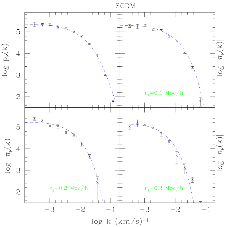
Figure 3: Auto-spectrum (top panel on the left) and three flux cross-spectra obtained with the definitions given in the text, for the SCDM model. The x-axis represents $\log k$, where $k$ is defined as $2\pi/v$, the y-axis is the log of auto-spectra and cross-spectra. The three cross-spectra have been obtained taking 10 QSO pairs whith three different proper separations ($0.1$ $h^{-1}$ Mpc, $0.2$ $h^{-1}$ Mpc, $0.3$ $h^{-1}$ Mpc). The dashed curve is the linear prediction of the 1D auto-spectrum and cross-spectrum as given in eq. (13) and in eq. (15). Error bars are the error of the mean value.

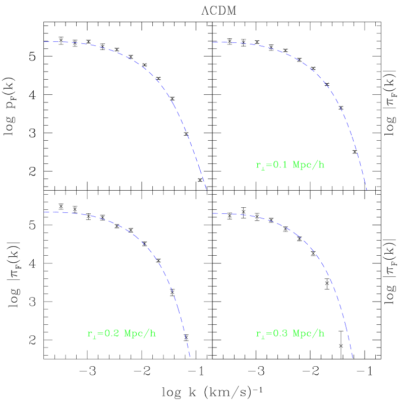
Figure 4: Same plot as in Figure 3 for a $\Lambda$CDM model

We compute the auto-spectra $p_{\cal F}(k)$ and the cross-spectra $\pi_{\cal F}(k|r_{\perp})$ of the flux for the two cosmological models using the definitions $p_{\cal F}(k)=\langle|{\cal F}_{0}(k)|^{2}\rangle$ and $\pi_{\cal F}(k|r_{\perp})=\langle Re\,({\cal F}_{0}(k){\cal F}_{1}^{*}(k,r_{\perp}))\rangle$, where ${\cal F}_{0}(k)$ and ${\cal F}_{1}(k)$ are the Fourier components of the flux along the two LOS at distance $r_{\perp}$ and the symbol $\langle\cdot\rangle$ denotes the ensemble average. In Figures 3 and 4 we plot the auto-spectrum (top panel on the left) and the three cross-spectra at proper distance $0.1$ $h^{-1}$ Mpc, $0.2$ $h^{-1}$ Mpc and $0.3$ $h^{-1}$ Mpc. The total number of simulated LOS pairs is 30. The results are ensemble averages of 10 pairs at each separation and the error bars represent the scatter of the mean value. The range of $k=2\pi/v$ ($v$ is the velocity in km/s) plotted here does not include the small scales (high $k$) strongly affected by pixel noise and non-linearity effects where the power spectra flattens again (Theuns, Haehnelt & Schaye 2000, McDonald et al. 2000). The dashed line represents the theoretical prediction of the linear power spectra as given by equation (15). The agreement is good over a wide range of wavenumbers $k$, roughly $-3\,\raise-2.0pt\hbox{\hbox to0.0pt{\hbox{$\sim$}\hss}\raise 5.0pt\hbox{$<$}\ }\log k\,\raise-2.0pt\hbox{\hbox to0.0pt{\hbox{$\sim$}\hss}\raise 5.0pt\hbox{$<$}\ }-1$. This is the interval we will use in Section 6 to recover the 3D power spectrum of the linear density field and is close to the range of k-wavenumbers used by Croft et al. (1999) from the analysis of observational data.

It is important here to stress that the simulated spectra have been produced in redshift-space, while the theory is in real-space. We have checked the difference by recomputing eq. (13) and eq. (15) considering also redshift-space distortions, i.e. using the distortion kernel proposed by Hui (1999), and the differences are negligible. Given this reasonably good agreement, all the following comparisons between the simulated spectra and the theory have been made without taking into account the redshift-space distortions in the theoretical equations.

We have also measured the flux cross-correlation coefficient $\chi(r_{\perp})$ as a function of separation, binning the data in bins with width $\Delta v$. We choose the following definition,

$$\chi(r_{\perp})=\frac{1}{N_{pix}}\frac{\sum_{i=1}^{N_{pix}}({\cal F}_{0}(i)-<{\cal F}_{0}>)({\cal F}_{1}(i)-<{\cal F}_{1}>)}{\sigma_{{\cal F}_{0}}\sigma_{{\cal F}_{1}}},$$ (30)

where ${\cal F}_{0}$ and ${\cal F}_{1}$ are the fluxes of the binned spectra of pairs with separation $r_{\perp}$, $N_{pix}$ is the number of pixels of the binned spectrum and $\sigma_{{\cal F}_{0}}$, $\sigma_{{\cal F}_{1}}$ the standard deviation of the two fluxes.

This function can be related to the auto and cross-spectra as follows,

$$\chi(r_{\perp})={\int_{0}^{\infty}dk~{}e^{-k^{2}/k_{\rm s}^{2}}\pi(k|r_{\perp})\over\int_{0}^{\infty}dk~{}e^{-k^{2}/k_{\rm s}^{2}}p(k)}\;,$$ (31)

where $k_{\rm s}^{-1}\propto(\Delta v)^{-1}$. Note that the flux cross-correlation coefficient does not depend on the amplitude but only on the shape of the power spectra. Using this function we can define a transverse coherence scale $r_{{\rm c}\perp}$ as the distance between two LOS at which $\chi(r_{{\rm c}\perp})=0.5$. Analytical estimates of $\chi(r_{\perp})$ for the various CDM models can be obtained by replacing $p$ and $\pi$ with the IGM linear density auto and cross-spectra $p_{11}$ and $\pi_{11}$ in the above relation.

We compare here three cosmological models, a SCDM, a $\Lambda$CDM and a $\tau$CDM model ($\Gamma\sim 0.2$) at seven angular distances (15, 30, 40, 55, 65, 80, 100 arcsec) at redshift $2.15$. This corresponds to different comoving distances $r_{\perp}$ in the three different cosmologies (e.g. Liske 2000),

$$r_{\perp}=\frac{c\,\theta}{H_{0}}\int_{0}^{z}\left[\Omega_{0m}(1+z^{\prime})^{3}+\Omega_{0\Lambda}\right]^{-1/2}\,d\,z^{\prime}\;\;\;\;\;$$ (32)

The IGM temperature at mean density and the temperature-density relation parameter are assumed to be $T_{0}=10^{4.2}$ K and $\gamma=1.3$, respectively.

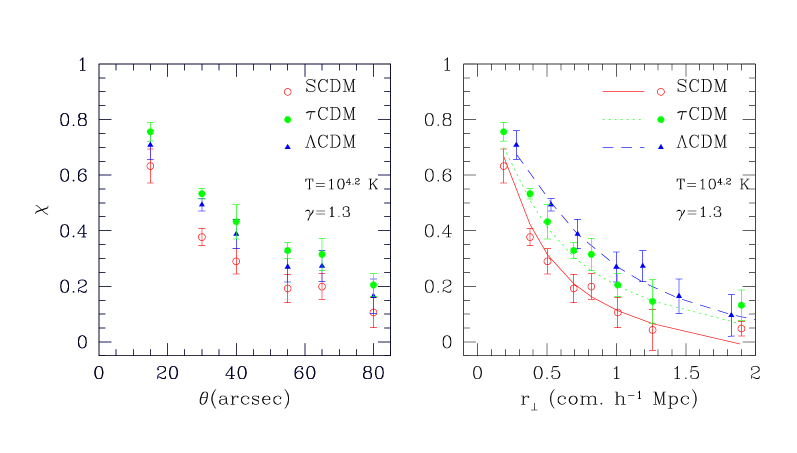
Figure 5: Cross-correlation coefficient $\chi$ plotted as a function of angular separation $\theta$ (left panel) and comoving separation $r_{\perp}$ (right panel). Points are the outputs of simulated QSO pairs for a SCDM (open circles) a $\tau$CDM with $\Gamma\sim 0.2$ (filled circles) and a $\Lambda$CDM model (triangles). The results are averaged over 8 pairs for each $\theta$ (15, 30, 40, 55, 65, 80). The curves in the right panel are the theoretical predictions of equation $(\ref{ccc_def})$. The dotted curve is for $\tau$CDM, the dashed is for $\Lambda$CDM while the solid curve is for SCDM. The error bars represent the scatter of the distribution.

We have generated 8 pairs of spectra for each angular separation in the usual way. The results are plotted in Figure 5 for the three models. The left and right panels show the cross-correlation coefficient against angular and comoving separation, respectively. The cross-correlation coefficient has been calculated directly from the whole spectrum (binned with $\Delta v\sim 3$ km s^-1). The three solid curves are calculated using equation $(\ref{ccc_def})$, where $\pi(k|r_{\perp})$ and $p(k)$ are replaced with the corresponding quantities for the IGM ($\pi_{11}$ and $p_{11}$). The agreement with the theoretical prediction (with $k_{s}\sim 2\pi/3$ km^-1 s) is reasonably good.

Using $\chi=0.5$ as the definition for the coherence length gives $0.10\pm 0.04$ $h^{-1}$ Mpc for SCDM, $0.13\pm 0.03$ $h^{-1}$ Mpc for $\tau$CDM and $0.17\pm 0.05$ $h^{-1}$ Mpc for $\Lambda$CDM (proper). The cross-correlation coefficient depends on the detailed shape of the IGM power spectrum at and above the Jeans length. In the SCDM model the power spectrum falls most steeply towards larger scales and this results in the shortest coherence length of the three models. The $\tau$CDM model with its flatter power spectrum on the relevant scales has a significatly larger coherence length. The $\Lambda$CDM model has an even larger coherence length due to the larger Jeans length for smaller $\Omega_{0m}$ at fixed temperature (eq. 2). However, the plot which can be directly compared with observations is the one on the left in Figure 5, which does not invoke any a priori assumption on the cosmological model. Unfortunately, the $\Omega_{0m}$ dependence becomes negligible if the cross-correlation coefficient is plotted against angular separation. The cross-correlation cofficient can, however, be used to constrain the shape of the DM power spectrum (which we have chosen here to paramerize with $\Gamma$) if the temperature $T_{0}$ and the temperature density relation coefficient $\gamma$ are determined indepedently.

We have also run simulations with a wider range of model parameters, changing $\Gamma$, $\Omega_{0m}$, $\sigma_{8}$ and the parameters describing the physics of the IGM, such as $T_{0}$, $\gamma$, $\Gamma_{-12}$. If $\tau_{eff}$ is fixed over the whole ensemble of simulations the dependencies on the amplitude of the power spectrum at that redshift and on $\Gamma_{-12}$ largely cancel.

The coherence length as defined above does not rely on assumptions about the shape of the absorbers. If the IGM indeed traces the filaments in the underlying dark matter distribution this should be a more adequate measure of the ‘characteristic size’ of the absorbers than the usually performed coincidence analysis of absorption lines fitted with a Voigt profile routine (see next section).

4 Coincidence analysis of Ly$\alpha$ absorption lines in QSO pairs

In this section we perform a coincidence analysis of absorption lines in the spectra along adjacent lines of sight (see Charlton et al. 1997 for a corresponding analysis of a hydrodynamical simulation). We have used the Voigt profile fitting routine AUTOVP (Davé et al. 1997) to identify and characterize the absorption lines. For this analysis we have generated absorption spectra of 5 QSO pairs in the range $1.9\leq z\leq 2.4$ for proper distances $0.05,0.1,0.2,0.4$ and $0.6$ $h^{-1}$ Mpc in the $\Lambda$CDM model only.

Charlton et al. (1997) demonstrated that for the filamentary and sheet-like absorping structures expected in hierachical structure formation scenarios the characteristic absorber ‘size’, as determined by counting ‘coincident’ and ‘anticoincident’ lines in QSO pairs, will depend on the separation of the QSO pair and on the column density threshold used. The characteristic size determined in this way is thus of little physical meaning and difficult to interpret. Nevertheless, such an analysis is useful in order to make connections with published observational studies which usually perform such an analysis.

Figure 6: The ratio of the number of coincidences to the number of coincidences plus anticoincidences, $f_{co}$, as a function of the proper separation of QSOs in $\Lambda$CDM model at a median redshift $z=2.15$. Left and right panel are for a velocity difference $\Delta v=50$ km/s and $\Delta v=150$ km/s, respectively. The three solid curves show $f_{co}$ for lines with a column density higher than $N_{\rm HI}=10^{12}$ cm^-2, $10^{13}$ cm^-2 and $10^{14}$ cm^-2 (from top to bottom). The three solid horizontal lines represent the level of random coincidences as estimated from $10$ pairs of uncorrelated LOS, for the same column density thresholds.

Figure 7: The same as in Figure 6 but at redshift $z=3$.

We adopt the definition of Charlton et al. (1997) based on the ‘hits-and-misses’ statistics described in McGill (1990). A coincidence is defined as the case in which an absorption line is present in both spectra within a given velocity difference $\Delta v$ and above some signal-to-noise ratio. An anticoincidence is defined when a line is present in one but not in the other spectrum. If there are two lines within $\Delta v$ we count only one coincidence and no anti-coincidence, as in Fang (1996). We also generate 5 uncorrelated LOS and compute the number of coincidences and anticoincidences in these 10 pairs to estimate the level of random coincidences.

In Figure 6 we plot the quantity $f_{co}$, the ratio of the number of coincidences to the sum of all coincidences and anticoincidences as a function of proper distance. The three curves are for different column density thresholds ($10^{12}$, $10^{13}$ and $10^{14}$ cm^-2) and the left and right panels are for $\Delta v=50,\,150$ km s^-1, respectively. The solid horizontal lines show the level of random coincidences as estimated from the ensemble average of $10$ uncorrelated spectra. The curves depend strongly on the choice of the velocity difference $\Delta v$.

In Figure 7 we plot the same quantities but for spectra with a median redshift $z=3$, i.e. the LOS span the range $2.75<z<3.25$. At fixed redshift, $f_{co}$ is larger if the velocity difference $\Delta v$ allowed for a coincidence is larger. This is easily understood as the chance to get a ‘hit’ becomes higher. There is also a significant trend with redshift. With increasing redshift both $f_{co}$ and the level of random coincidences increase, the latter by a factor of two. These findings are similar to those of Charlton et al. (1997) (their Figure 2). Our level of random coincidences is somewhat smaller than that in Charlton et al. (1997), probably due to a different temperature which results in a larger Jeans scale.

Figure 8: Column density of neutral hydrogen, $\log N_{\rm HI}$, for pairs of coincident absorption lines identified with the Voigt profile fitting routine AUTOVP in a $\Lambda$CDM model at $z=2.15$. A velocity difference of $\Delta v=50$ km/s was allowed for coincident lines. Four different proper separations are shown: $r_{\perp}=0.05$ $h^{-1}$ Mpc, top left panel; $r_{\perp}=0.1$ $h^{-1}$ Mpc, top right panel; $r_{\perp}=0.2$ $h^{-1}$ Mpc, bottom left panel and $r_{\perp}=0.4$ $h^{-1}$ Mpc, bottom right panel.

In Figure 8 we show scatter plots of the neutral hydrogen column densities of coincident lines above a column density threshold of $10^{12}\rm cm^{-2}$. For the smaller separations the column densities are well correlated while for larger distances the column density difference rapidly increases. This is again not surprising as for large separations the ‘coincidences’ occur mostly by chance. The same analysis has been done for lines found at $z=3$. The result is very similar to the one found at $z=2.15$.

The results presented in this section depend on details of the Voigt profile fitting and the velocity difference and column density threshold chosen to do the ‘hits-and-misses’ statistics. This makes it difficult to infer physically meaningful properties of the absorbers, as for example their characteristic size, with these techniques. The coherence length defined in the last section is more useful in this respect.

5 Recovering the 3D dark matter power spectrum using flux cross-spectra

5.1 A new method for obtaining the 3D dark matter spectrum from the flux auto-spectrum

If the effect of peculiar velocities, thermal broadening and instrumental noise on the flux fluctuations at small scales are neglected the transmitted flux at redshift $z$ in a given direction ${\hat{\theta}}$ can be approximated as (e.g. Croft et al. 1998; Theuns et al. 1999)

$${\cal F}({\hat{\theta}},z)=\exp\left[-A\left(1+\delta^{\rm IGM}\left({\bf x}({\hat{\theta}},z),z\right)\right)^{\beta}\right]\;,$$ (33)

where $\beta\approx 2-0.7(\gamma-1)$, while $A$ is a normalization constant of order unity which determines the mean flux in the considered redshift interval. Eq. (33) is valid only in redshift-space and the effect of peculiar velocity and thermal broadening increases the scatter in the relation between ${\cal F}$ and $\delta^{\rm IGM}$ (Croft et al. 1998).

If smoothed on a sufficiently large scale the IGM overdensity can be treated as a linearly fluctuating field. In this case the fluctuations of the flux, $\delta{\cal F}$, are simply related to the linear baryon density perturbations,

$$\delta{\cal F}({\hat{\theta}},z)\approx-A\beta\delta_{0}^{\rm IGM}\left({\bf x}({\hat{\theta}},z),z\right)\;.$$ (34)

Figure 9: $\pi_{F}$ as a function of $r_{\perp}$ (in proper $h^{-1}$ Mpc at $z=2.15$) for 4 different values of $k$: $k=0.169,0.561,1.005,1.806$ Mpc^-1 for SCDM model (left panel, from top to bottom) and $k=0.125,0.414,0.742,1.333$ Mpc^-1 for the $\Lambda$CDM model (right panel, from top to bottom). The dashed curve is the theoretical prediction given by eq. (15), not corrected for redshift-space distortions. The points are calculated for an ensemble of 30 realizations, 10 realizations for each separation: $r_{\perp}=0$ $h^{-1}$ Mpc (which gives the auto-spectrum) and $r_{\perp}=0.1,0.2,0.3$ $h^{-1}$ Mpc.

On large scales observed absorption spectra can thus be used to recover the 3D primordial power spectrum of DM perturbations. The standard procedure suggested by Croft et al. (1998, 1999, 2000) inverts the relation in eq. (13) to obtain the 3D power spectrum by differentiating the 1D auto-spectrum,

$$P(k)=-{2\pi\over k}{d\over dk}p(k)\;.$$ (35)

Alternative methods to measure the amplitude of DM fluctuations and their power spectrum have been proposed by Hui (1999) and by Nusser & Haehnelt (1999, 2000).

However, the 3D power spectrum can also be reconstructed by integrating the 1D cross-spectrum $\pi(k|r_{\perp})$ over the transverse separation between LOS pairs. Indeed, by inverse Fourier transforming eq. (11) on the plane spanned by ${\bf r}_{\perp}$, and integrating over angles, we find

$$P(k)=2\pi\int_{0}^{\infty}dr_{\perp}r_{\perp}J_{0}(r_{\perp}\sqrt{k^{2}-q^{2}})~{}\pi(q|r_{\perp})\equiv\int_{0}^{\infty}{dr_{\perp}\over r_{\perp}}~{}{\cal Q}(r_{\perp}|k,q)\;,\ \ \ \ \ \ \ \ q\leq k\;.$$ (36)

The above results also lead to a useful ‘consistency relation’ between the LOS auto-spectrum $p(k)$ and the cross-spectra $\pi(k|r_{\perp})$ along LOS pairs,

$$\pi(k|r_{\perp})=p(k)-r_{\perp}\int_{0}^{\infty}dqJ_{1}(qr_{\perp})p\left(\sqrt{q^{2}+k^{2}}\right)\;.$$ (37)

As a consequence of the assumed homogeneity and isotropy, the RHS of equation (36) does not depend on $q$; we can therefore simplify the integral by taking $q=k$,

$$P(k)=2\pi\int_{0}^{\infty}dr_{\perp}r_{\perp}\pi(k|r_{\perp})\;.$$ (38)

The flux cross-spectrum $\pi_{F}(k|r_{\perp})$ is plotted in Figure 9 as a function of $r_{\perp}$ for a SCDM (left panel) and a $\Lambda$CDM (right panel) model, from an ensemble of 30 pairs at different separations. The different set of points are for different values of $k$ in the range for which the agreement with theoretical predictions is good. The $r_{\perp}=0$ $h^{-1}$ Mpc point which represents the auto-spectrum is also shown. The 3D power spectrum can be obtained using eq. (38). To estimate $P(k)$ we can use the values of $\pi_{F}(k|r_{\perp})$ obtained from the simulations in the analytical expression. Also in this case the reconstruction procedure is based on eqs. which neglect the effects of redshift-space distortions, while the spectra have been produced in redshift space.

More generally the redundancy shown by the $q$-dependence of the integrand in the RHS of eq. (36) can be exploited to choose a weighting such that the dominant contribution to the integral comes from the separation range where the signal-to-noise ratio and/or the number of observed pairs is highest.

Figure 10: $Q$ as a function of ln(r_⟂) in $\Lambda$CDM model for three values of $k$: $k=0.1251,0.4142,0.7422$ Mpc^-1 (from top to bottom) and for two choices of $q$: $q=k$ in the left panel and $q=k/3$ in the right panel.

This point is made more clear by Figure 10, where the quantity ${\cal Q}$ is plotted as a function of the transverse separation $r_{\perp}$ for various values of $k$ and $q$. In Figure 10 the solid curves show the theoretical predictions for ${\cal Q}$ in a $\Lambda$CDM Universe: in the left panel for $q=k$; in the right panel for $q=k/3$. It is evident that the behaviour is very different: for $q=k$ the Bessel function ${\rm J_{0}}$ is equal to 1, while for $q=k/3$ it acts as a filter which takes both positive and negative values.

To simplify matters we dropped the explicit redshift dependence of the power spectra in the above discussion and used power spectra which were averaged over some redshift interval. The recovered 3D power spectrum will then generally depend on the median redshift of that interval. Moreover, the assumed isotropy is generally broken, e.g. due to the effect of peculiar velocities. A more refined treatment should thus account for various sources of anisotropy in the reconstruction procedure by applying for example the techniques proposed by Hui (1999), McDonald & Miralda-Escudé (1999) and Hui et al. (1999). These and other aspects of the power spectrum reconstruction will be discussed elsewhere.

A reconstruction procedure for the DM power spectrum based on eqs. (36) or (38) has an obvious advantage over the standard method based on eq. (35): one integrates rather than differentiates a set of generally noisy data. To investigate this we have performed the reconstruction of the initial 3D power spectrum in three different ways:

• differentiation of simulated 1D auto-spectra, based on eq. (35);

• integration of 1D cross-spectra, recovered from simulated 1D auto-spectra, based on eqs. (37) and (38);

• fitting of simulated 1D cross-spectra, based on eq. (12).

At first we generate 15 LOS and then compute the flux auto-spectra. We choose to smooth the auto-spectra with a polynomial function before using eq. (35) to recover the 3D power spectrum. In panel $(a)$ of Figure 11 one can see that the agreement with the theoretical prediction is good over a wide range of wave-numbers. The error bars represent the scatter over the distribution of the 15 recovered 3D power spectra. Almost all the $1\sigma$ error bars of the points match the continuous line which represents the 3D linear IGM power spectrum. We stress the fact that this technique has been used ‘directly’ on simulated fluxes, without the use of further assumptions, such as Gaussianization (e.g. Croft et al. 1998).

In panel $(b)$ of Figure 11 we report the results obtained with the second technique based on equations (37) and (38), using only the auto-spectra information. For each of the 15 flux auto-spectra we compute the cross-spectra for a large number of separations via eq. (37). Next we use these estimates in eq. (38), i.e. we integrate the 1D flux cross-spectra along the transverse direction. The agreement with linear theory of this ‘integration’ technique is very good. In this panel the error bars represent the scatter over the distribution of recovered 3D power spectra. The results obtained with these two techniques are basically equivalent provided we smooth the simulated data. In a sense this method provides a natural choice of a smoothing function. If we apply these two methods directly without any smoothing then ‘differentiation’ is less accurate in recovering the 3D dark matter power spectrum at large scales and ‘integration’ produces smaller error bars. Another significant result is that both methods fail to recover the 3D dark matter power spectrum for large wave-numbers ($k\,\raise-2.0pt\hbox{\hbox to0.0pt{\hbox{$\sim$}\hss}\raise 5.0pt\hbox{$>$}\ }0.1$ km^-1 s): at small scales, peculiar velocities, thermal broadening and nonlinear gravitational effects are responsible for a drop of the flux power spectrum below that predicted by linear theory.

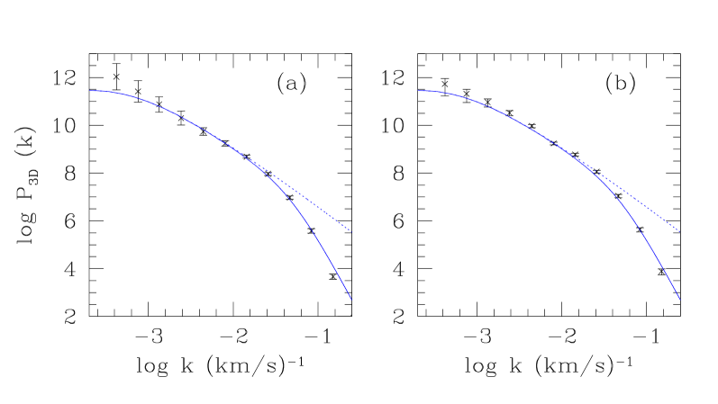
Figure 11: 3D power spectrum reconstruction. In panel $(a)$ points represent the 3D power spectrum obtained with ‘differentiation’, i.e. using eq. (35). In panel $(b)$ points represent the same quantity obtained with ‘integration’, i. e. using eqs. (37) and (38). The dotted curve is the 3D power spectrum of the dark matter, while the solid curve is the 3D power spectrum of the IGM.

Our third method uses eq. (12): we fit the simulated cross-spectra with a $\Lambda$CDM power spectrum with the amplitude as a free parameter and determine the best estimate of the amplitude by $\chi^{2}$ minimization. We thereby fitted only the part at small wave-numbers (scales larger than few Mpc) less affected by non-linear effects, peculiar velocities and Jeans length smoothing. A further advantage of using the cross-spectra is that in a set of N auto-spectra, there are $N\times(N-1)/2$ cross-spectra, so this second sample could in principle be significantly larger than the first. We proceed as follows. First we calculate the error in estimating the amplitude of the 3D power spectrum by using only 5 flux auto-spectra. Then, having generated a set of QSO pairs with given separations, we determine the minimum number of QSO pairs needed to recover the amplitude with the same accuracy and with a mean value compatible within $1\sigma$ with the amplitude recovered from the 5 flux auto-spectra. We find that from a set of 5 simulated flux auto-spectra it is possible to determine the logarithm of the amplitude with an accuracy of $1\%$. We find that at large separations one needs more pairs to give an accurate estimate of the amplitude. For separations smaller than 2 comoving Mpc we need less than 10 QSO pairs to reach the same accuracy and the same amplitude of the auto-spectra estimate. A detailed method that recovers not only the amplitude but also the slope of the 3D power spectrum, based on eq. (12) will be described in a future paper.

We conclude from our comparison that with the ‘integration’ technique the correct slope of 3D dark matter power spectrum can be inferred on scales larger than 1 comoving Mpc. This method is complementary to the usual ‘differentiation’ and is very accurate. Our ‘fitting’ technique for the flux cross-spectra of a set of QSO pairs can also constrain the 3D power spectrum.

5.2 Cross-spectra as a means of overcoming limitations of auto-spectra due to continuum fitting

As discussed by Croft et al. (1998, 2000) and Hui et al. (2000), at scales $k<0.005$ km^-1 s corresponding to about $10-15\,h^{-1}$ Mpc the errors in observed 3D flux auto-spectra as determined by a bootstrap analysis increase rapidly. Errors in the continuum fitting procedure are likely be the main contributor. In principle such continuum fitting errors can both increase or decrease the amplitude of the flux auto-spectrum.

Cross spectra should in principle not be affected by any modulation of the flux which is uncorrelated between adjacent LOS even though the shot noise will increase with increasing fluctuation amplitude. Continuum fitting should thus affect flux cross-spectra much less than flux auto-spectra.

In this subsection we verify that this is indeed the case and assess how many quasar pairs are needed to extend measurements of the DM spectrum to scales as large as $60\,h^{-1}$ Mpc or more. We first mimic the effect of errors in the continuum fitting procedure on flux auto and cross-spectra and then go on to demonstrate explicitly that continuum fitting may actually not be necessary for the analysis of flux cross-spectra.

To mimic the effect of continuum fitting errors we do the following. We take the continuum of the QSO $Q1422+231$ kindly provided by Michael Rauch (Rauch et al. 1997). From this we generate a series of spectra with continuum fitting errors by changing the amplitude of the Fourier modes of our analytical spectra at all k corresponding to scales larger than 15 comoving Mpc, i.e. the scales most likely affected by errors in the continuum fitting procedure. We add to the old amplitude a quantity which varies randomly between $-$ 10 % to 10 % of the amplitude of the corresponding Fourier mode of the continuum of $Q1422+231$. Then we calculate a new spectrum keeping all the phases of the Fourier modes of these continua in order to preserve the characteristic emission lines of the continuum of $Q1422+231$. We also shift the spectrum randomly in redshift to avoid correlations due to the charateristic emission lines. Similarly we produce spectra with different independent continua by randomly varying the large scale Fourier modes of the continuum of $Q1422+231$ by $\pm$ -15 %. In the following we will refer to the first set of spectra as the no continuum case and to the second as the continuum case. We have simulated spectra of 30 QSO pairs in a $\Lambda$CDM Universe with an angular separation of 100 arcsec in this way.

Examples of spectra of three QSO pairs with ‘continuum fitting errors’ are shown in Figure 12 (no continuum case). Our ‘continuum fitting errors’ are clearly visible by eye and are significantly larger than those that should be achievable with a careful continuum fitting procedure.

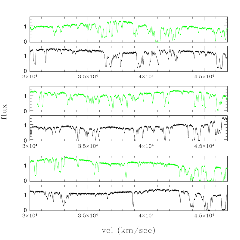
Figure 12: Spectra from three QSO pairs with continuum errors added as described in the text

We have computed flux cross-spectra and auto-spectra for the two samples. The results are reported in Figure 13, where we plot the value of the flux cross-spectra and auto-spectra computed from a given number of pairs, at two fixed values of $k=5\times 10^{-4}$ km^-1 s (left panels) and $k=10^{-3}$ km^-1 s (right panels). These correspond to scales of $60$ and $120\,h^{-1}$ Mpc, respectively. The upper panels refer to the no continuum case and the bottom ones to continuum one.

In all four cases shown here the flux auto-spectra (points) give values significantly larger than those of the linear prediction (dotted line), as determined by eq. (13). The flux cross-spectra (triangles), however, converge to the right mean value (continuous line) obtained from eq. (15), although the number of pairs needed is not small. This is due to the fact that the fluctuations in the continua of the QSO eventually cancel out when the spectra are cross-correlated, while they add in quadrature to the flux auto-spectrum.

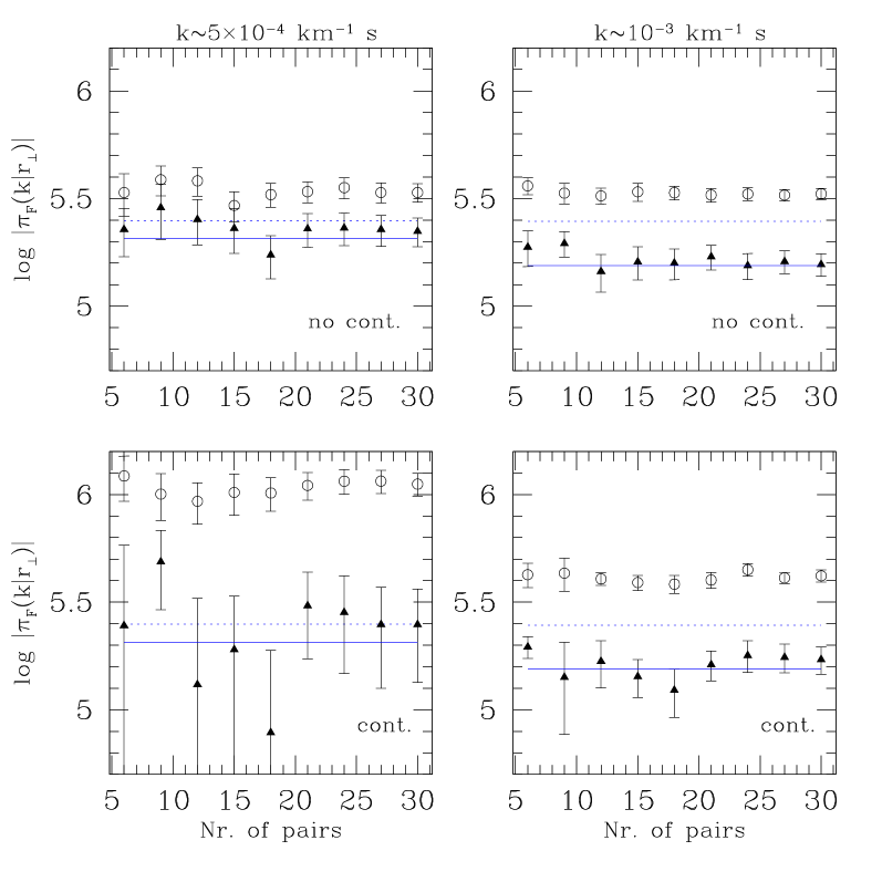
Figure 13: Flux cross-spectra (triangles) vs. number of QSO pairs. Points represent the flux auto-spectra. The solid curve is the theoretical prediction for the IGM linear density cross-spectrum, eq. (15), while the dotted curve is the theoretical prediction for the IGM linear density auto-spectrum, eq. (13). The left panels are for $k=5\times 10^{-4}$ km^-1 s, corresponding to a scale of about $60\,h^{-1}$ Mpc; the right panels are for $k=10^{-3}$ km^-1 s, corresponding to a scale of about 120 $h^{-1}$ Mpc. The upper panels refer to the no continuum case, in which no continuum is present and we mimic the errors introduced by the continuum-fitting. The bottom panels refer to the continuum case, in which we directly cross-correlate spectra without removing the continuum. Error bars are the error of the mean values.

The variations of the flux cross-spectrum around the mean value are due to the combined effect of cosmic variance and the shot noise due to the continuum fitting errors and the continuum fluctuations, respectively. At $k=10^{-3}$ km^-1 s the 1D flux cross-spectrum can be obtained with an accuracy of 2% in logarithmic units from 30 QSO pairs in both the continuum and the no continuum case. It should thus be possible to constrain the rms fluctuation amplitude of the matter density at scales of $60\,h^{-1}$ Mpc with an accuracy of about 15%. Such a measurement should not require continuum fitting. At even larger scale the errors for the continuum case start to blow up with 30 QSO pairs. A larger number of pairs would be required to beat down the shot noise.

Attempts to recover the 3D power spectrum on large scales using the flux auto-spectra clearly do not determine the correct value if continuum fitting errors are present. As demonstrated above it should, however, be possible to overcome this limitation by the use of flux cross-spectra.

A simple method to recover the right power spectrum for small wave-numbers could be based on eq. (12). We can parametrize the power spectrum and then compute the cross-spectra with $r_{\perp}$ equal to the separation of the pairs. The slope of the power spectrum at large scales can then be constrained by $\chi^{2}$ minimization. A more detailed discussion on the use of 1D cross-spectra for the determination of the DM power spectrum on all scales will be presented elsewhere.

6 Discussion and conclusions

We have presented an effective implementation of analytical calculations of the Ly$\alpha$ opacity distribution of the Intergalactic Medium (IGM) along multiple lines of sight (LOS) to distant quasars in a cosmological setting. We thereby assumed that the neutral hydrogen distribution traces the dark matter distribution on scales larger than the Jeans length of a warm photoionized IGM. Simulated absorption spectra with varying transverse separation between different LOS have been investigated. We have identified coincident absorption features as fitted with a Voigt profile fitting routine and calculated the cross-correlation coefficient and the cross-power spectrum of the flux distribution along different LOS to quantify the flux correlation.

As expected the correlation of the flux along adjacent LOS is sensitive to the detailed shape of the power spectrum on scales at and above the Jeans length. We have studied the dependence of the cross-correlation coefficient on the shape parameter $\Gamma$ of the assumed CDM model and on the Jeans scale which determines the small-scale cut-off of the power spectrum of the gas distribution due to pressure of the gas. We have confirmed previous results that the characteristic size of the absorbers inferred from simple hit-and-miss statistics of fitted absorption lines assuming spherical absorbers depends strongly on the column density threshold used and on the separation of the QSO pairs. This reiterates the point that the filamenatary and sheetlike distribution of the IGM suggested by numerical simulations makes the concept of spherical absorbers with a characteristic size of very limited use. Nevertheless, we obtain values which are in reasonable agreement with those derived from observations of multiple systems by Crotts & Fang (1998), Petitjean et al. (1998), D’Odorico et al. (1998), Young et al. (2000).

The cross-correlation coefficient can be used to define a ‘characteristic’ correlation length of the absorbers in a more objective way. We obtain $0.10\pm 0.04$ $h^{-1}$ Mpc for SCDM, $0.13\pm 0.03$ $h^{-1}$ Mpc for $\tau$CDM and $0.17\pm 0.05$ $h^{-1}$ Mpc for $\Lambda$CDM (all at $z=2.15$) as the scale where the cross-correlation coefficient falls to 0.5. This is about the Jeans length of the IGM at this redshift. We demonstrate that if the temperature and the slope of the temperature density relation can be determined indepedently then the cross-correlation coefficient can be used to constrain the shape parameter $\Gamma$ in a way which is independent of the amplitude of the power spectrum.

We furthermore propose a new technique to recover the 3D linear dark matter power spectrum by integrating over 1D flux cross-spectra. This method is complementary to the usual ‘differentiation’ of 1D auto-spectra and suffers different systematic errors. It can be used for the calculation of the cross-power spectrum from a given set of auto-power spectra. We show that it is mathematically equivalent to the usual ‘differentiation’ but offers a natural way of smoothing the data in the presence of noise.

The biggest advantage of the cross-correlation of the flux distribution of adjacent lines is its ability to eliminate errors which are uncorrelated in different LOS. The erroneous flux fluctuations introduced by the continuum fitting procedure, which is necessary to remove the non-trivial wave-length dependence of the quasar emission, are such an error which is largely uncorrelated. We demonstrate that, as expected, such uncorrelated errors affect the cross-power spectrum significantly less than the auto-power spectrum. This may render the tedious and somewhat arbitrary continuum fitting procedure unnecessary for the recovery of the dark matter power spectrum from the flux correlations in adjacent LOS.

Continuum fitting errors have been the main limitation of using flux auto-power spectra to constrain the DM power spectrum at scales larger than about $10h^{-1}$Mpc. When flux correlations of adjacent LOS are used the errors at large scales will be dominated by cosmic variance, residuals in the removal of the effect of peculiar velocities, the uncertainty in the temperature density relation, and possible temperature fluctuations of the IGM which result in opacity fluctuations due to the temperature dependence of the recombination coefficient. The errors due to cosmic variance and peculiar velocities will decrease with increasing number of LOS and flux correlations should thus allow to extend studies of the DM power spectrum with the Ly$\alpha$ forest to significant larger scale than is possible with flux auto-power spectra. We estimate that 30 pairs with separation of 1-2 arcmin are necessary to determine the 1D cross-spectrum at scales of $60\,h^{-1}$ Mpc, with an accuracy of about 30% if the error is dominated by cosmic variance.

References

- [] Alcock C., Paczyński B., 1979, Nature, 281, 358
- [] Bahcall J.N., Salpeter E.E., 1965, ApJ, 142, 1677
- [] Bahcall J.N., Sarazin C.L., 1978, ApJ, 219, 781
- [] Bardeen J.M., Bond J.R., Kaiser N., Szalay A.S., 1986, ApJ, 304, 15
- [] Bechtold J., Crotts A.P.S., Duncan R.C., Fang Y., 1994, ApJ, 437, L83
- [] Bi H.G., 1993, ApJ, 405, 479
- [] Bi H.G., Börner G., Chu Y., 1992, A&A, 266, 1
- [] Bi H.G., Davidsen A.F., 1997, ApJ, 479, 523
- [] Bi H.G., Ge J., Fang L.-Z., 1995, ApJ, 452, 90
- [] Bond J.R., Kofman L., Pogosyan D., 1996, Nature, 380, 603
- [] Cen R., Miralda-Escudé J., Ostriker J.P., Rauch M., 1994, ApJ, 437, L83
- [] Charlton J.C., Anninos P., Zhang Y., Norman M.L., 1997, ApJ, 485, 26
- [] Coles P., Jones B., 1991, MNRAS, 248, 1
- [] Croft R.A.C., Weinberg D.H., Katz N., Hernquist L., 1998, ApJ, 495, 44
- [] Croft R.A.C., Weinberg D.H., Pettini M., Hernquist L., Katz N., 1999, ApJ, 520, 1
- [] Croft R.A.C., Weinberg D.H., Bolte M., Burles S., Hernquist L., Katz N., Kirkman D., Tytler D., 2000, ApJ, submitted, astro-ph/0012324
- [] Crotts A.P.S., Fang Y., 1998, ApJ, 502, 16
- [] Davé R., Hernquist L., Weinberg D.H. , Katz N., 1997, ApJ, 477, 21
- [] Dinshaw N., Foltz C.B., Impey C.D., Weymann R.J., Morris S.L., 1995, Nature, 373, 223
- [] Dinshaw N., Impey C.D., Foltz C.B., Weymann R.J., Chafee F.H., 1994, ApJ, 437, L87
- [] Dinshaw N., Weymann R.J., Impey C.D., Foltz C.B., Morris S.L., Ake T., 1997, ApJ, 491, 45
- [] D’Odorico V., Cristiani S., D’Odorico S., Fontana A., Giallongo E. Shaver P., 1998, A&A, 339, 678
- [] Efstathiou G., Schaye J., Theuns T., 2000, Philosophical Transactions of the Royal Society, Series A, Vol. 358, no. 1772,p. 2049
- [] Fang Y., Duncan R.C., Crotts A.P.S., Bechtold J., 1996, ApJ, 462, 77
- [] Feng L.-L., Fang L.-Z., 2000, preprint astro-ph/0001348
- [] Foltz C.B., Weymann R.J., Röser H.-J., Chaffee F.H., 1984, ApJ, 281, L1
- [] Gnedin N.Y., Hui L., 1996, ApJ, 472, L73
- [] Gnedin N.Y., Hui L., 1998, MNRAS, 296, 44
- [] Gunn J.E., Peterson B.A., 1965, ApJ, 142, 1633
- [] Hernquist L., Katz N., Weinberg D.H., Miralda-Escudé J., 1996, ApJ, 457, L51
- [] Hui L., 1999, ApJ, 516, 525
- [] Hui L., Gnedin N.Y., Zhang Y., 1997, ApJ, 486, 599
- [] Hui L., Stebbins A., Burles S., 1999, ApJ, 511, L5
- [] Hui L., Burles S., Seljak U., Rutledge R. E., Magnier E., Tytler D., 2000, preprint astro-ph/0005049
- [] Kim T.-S., Cristiani S., D’Odorico S., 2001, preprint astro-ph/0101005
- [] Lahav O., Lilje P.B., Primack J.R., Rees M.J., 1991 MNRAS, 251, 128
- [] Liske J., 2000, MNRAS, 319, 557
- [] Liske J., Webb J.K., Williger G.M., Fernández-Soto A., Carswell R.F., 2000, MNRAS, 311, 657
- [] Lumsden, S. L., Heavens, A. F., Peacock, J. A., 1989, MNRAS, 238, 293
- [] Matarrese S., Mohayaee, R., 2001, preprint astro-ph/0102220
- [] McDonald P., Miralda-Escudé J., 1999, ApJ, 518, 24
- [] McDonald P., Miralda-Escudé J., Rauch M., Sargent W.L.W., Barlow A., Cen R., Ostriker J.P., 2000, ApJ, 543, 1
- [] McGill C., 1990, MNRAS, 242, 544
- [] Meiksin A., 1994, ApJ, 431, 109
- [] Miralda-Escudé J., Rees M., 1994, MNRAS, 266. 343
- [] Miralda-Escudé J., Cen R., Ostriker J.P., Rauch M., 1996, ApJ, 471, 582
- [] Narayanan V.K., Spergel D.N., Davé R., Ma C.P., 2000, preprint astro-ph/0001247
- [] Nusser A., 2000, MNRAS, 317, 902
- [] Nusser A., & Haehnelt M., 1999, MNRAS, 303, 179
- [] Nusser A., & Haehnelt M., 2000, MNRAS, 313, 364
- [] Petitjean P., Surdej J., Smette A., Shaver P., Mücket J., Remy M., 1998, A&A, 334, L45
- [] Porciani C., Matarrese S., Lucchin F., Catelan P., 1998, MNRAS, 298, 1097
- [] Rauch M., 1998, ARA&A, 36, 267
- [] Rauch M., Haehnelt M., 1995, MNRAS, 275L, 76R
- [] Rauch M., Sargent W.L.W. Barlow, T.A., 1999, ApJ, 515, 500
- [] Rauch M., Miralda-Escude J., Sargent W. L. W., Barlow T. A., Weinberg D. H., Hernquist L., Katz N., Cen R., Ostriker J. P., 1997, ApJ, 489, 7
- [] Reisenegger A., Miralda-Escudé J., 1995, ApJ, 449, 476
- [] Roy Choudhury T., Padmanabhan T., Srianand R., MNRAS, 2001, 322, 561
- [] Roy Choudhury T., Srianand R., Padmanabhan T., 2001, MNRAS, submitted, preprint astro-ph/00012498
- [] Schaye J., Theuns T., Rauch M., Efstathiou G., Sargent W.L.W., MNRAS, 2000, 318, 817
- [] Smette A., Robertson J.G., Shaver P.A., Reimers D., Wisotzki L., Köhler Th., 1995, A&AS, 113, 199
- [] Smette A., Surdej J., Shaver P.A., Foltz C.B., Chaffee F.H., Weymann R.J., Williams R.E., Magain P., 1992, ApJ, 389, 39
- [] Sugiyama N., 1995, ApJS, 100, 281
- [] Theuns T., Schaye J., Haehnelt M.G., 1999, MNRAS, submitted, preprint astro-ph/9908288
- [] Theuns T., Leonard A., Efstathiou G., Pearce F.R., Thomas P.A., 1998, MNRAS, 301, 478
- [] Williger G.M., Smette A., Hazard C., Baldwin J.A., McMahon R.G., 2000, ApJ, 532, 77
- [] White M., Croft R.A.C., 2000, preprint astro-ph/0001247
- [] Young P. A., Impey C. D., Foltz, C. B., 2000, preprint astro-ph/0010058
- [] Zel’dovich ya. B., 1970, A&A, 5, 84
- [] Zhang Y., Anninos P., Norman M.L., 1995, ApJ, 453, L57
- [] Zhang Y., Anninos P., Norman M.L., Meiksin A., 1997, ApJ, 485, 496
- [] Zhang Y., Meiksin A., Anninos P., Norman M.L., 1998, ApJ, 495, 63