Ultra-high energy cosmic rays from
annihilation of superheavy dark matter

Abstract

We consider the possibility that ultra-high energy cosmic rays originate from the annihilation of relic superheavy dark matter. We find that a cross section of $\langle\sigma_{A}v\rangle\sim 10^{-26}\textrm{cm}^{2}(M_{X}/10^{12}\,\textrm{GeV})^{3/2}$ is required to account for the observed rate of super-GZK events if the superheavy dark matter follows a Navarro–Frenk–White density profile. This would require extremely large-$l$ contributions to the annihilation cross section. We also calculate the possible signature from annihilation in sub-galactic clumps of dark matter and find that the signal from sub-clumps dominates and may explain the observed flux with a much smaller cross section than if the superheavy dark matter is smoothly distributed. Finally, we discuss the expected anisotropy in the arrival directions of the cosmic rays, which is a characteristic signature of this scenario.

, , and

1 Introduction

The nature of the dark matter and the origin of the ultra-high energy (UHE) cosmic rays are two of the most pressing issues in contemporary particle astrophysics. In this paper we explore a possible connection between these issues: dark matter is a very massive relic particle species (wimpzilla), and wimpzilla annihilation products are the ultra-high energy cosmic rays.

The dark matter puzzle results from the observation that visible matter can account only for a small fraction of the matter bound in large-scale structures. The evidence for dark matter is supported by mass estimates from gravitational lensing [1], by the peculiar velocities of large scale structures [2], by measurements of CMB anisotropy [3] and by measurements of the recession velocity of high-redshift supernovae [4]. Constraints from big-bang nucleosynthesis imply that the bulk of the dark matter cannot be baryonic, and most of the matter density of the universe must arise from particles not accounted for by the Standard Model of particle physics [5].

The existence of UHE cosmic rays of energies above the Greisen-Zatsepin-Kuzmin cutoff [6], $E_{\mathrm{GZK}}\simeq 5\times 10^{19}\,$eV, is a major puzzle because the cosmic microwave background constitutes an efficient obstacle for protons or nuclei of ultra-high energies to travel farther than a few dozen Mpc [6, 7]. This suggests that the observed extremely energetic cosmic rays with $E>E_{\mathrm{GZK}}$ should originate in our cosmic neighborhood. Furthermore, the approximately isotropic distribution of arrival directions makes it difficult to imagine that nearby astrophysical sources are the accelerators of the observed UHE cosmic rays (but for the opposite point of view, see [8]).

An interesting possibility is that UHE cosmic rays arise from the decay of some superheavy particle. This possibility has been proposed by Berezinsky, Kachelrieß and Vilenkin and by Kuzmin and Rubakov [9, 10], see also [11] for a discussion of this in the framework of string/M-theory, and [12] for a discussion in the framework of topological defects. The superheavy particles must have masses $M_{X}\geq 10^{12}\,$GeV. Although this proposal circumvents the astronomical problems, there are two issues to address: Some cosmological mechanism must be found for producing particles of such large mass in the necessary abundance, and the lifetime of this very massive state must be in excess of $10^{20}\,$yr, if we want these particles to be both dark matter candidates and sources of UHE cosmic rays.

The simple assumption that dark matter is a thermal relic limits the maximum mass of the dark matter particle. The largest annihilation cross section in the early universe is expected to be roughly $M_{X}^{-2}$. This implies that very massive wimps have such a small annihilation cross section that their present abundance would be too large if the wimps are thermal relics. Thus, one predicts a maximum mass for a thermal wimp, which turns out to be a few hundred TeV. While a thermal origin for wimps is the most common assumption, it is not the simplest possibility. It has been recently pointed out that dark particles might have never experienced local chemical equilibrium during the evolution of the universe, and that their mass may be in the range $10^{12}$ to $10^{19}$ GeV, much larger than the mass of thermal wimps [13, 14, 15, 16]. Since these wimps would be much more massive than thermal wimps, such superheavy dark particles have been called wimpzillas [16].

Since wimpzillas are extremely massive, the challenge lies in creating very few of them. Several wimpzilla scenarios have been developed involving production during different stages of the evolution of the universe.

wimpzillas may be created during bubble collisions if inflation is completed through a first-order phase transition [17, 18]; at the preheating stage after the end of inflation with masses easily up to the Grand Unified scale of $10^{15}$GeV [19] or even up to the Planck scale [20, 21, 22]; or during the reheating stage after inflation [15] with masses which may be as large as $2\times 10^{3}$ times the reheat temperature.

wimpzillas may also be generated in the transition between an inflationary and a matter-dominated (or radiation-dominated) universe due to the “nonadiabatic” expansion of the background spacetime acting on the vacuum quantum fluctuations. This mechanism was studied in details in Refs. [13, 23, 24]. The distinguishing feature of this mechanism is the capability of generating particles with mass of the order of the inflaton mass (usually much larger than the reheat temperature) even when the particles only interact extremely weakly (or not at all) with other particles, and do not couple to the inflaton.

The long lifetime required in the decay scenario for UHE cosmic rays is problematic if the UHE cosmic rays originate in single-particle decays. The lifetime problem can be illustrated in the decays of string or Kaluza–Klein dilatons. These particles can be decoupled from fermions [25], and therefore decay in leading order through their dimension-five couplings to gauge fields

$$\mathcal{L}_{I\Phi}=-\frac{\Phi}{4f}\ F^{\mu\nu}{}_{a}F_{\mu\nu}{}^{a}.$$ (1)

Here, $f$ is a mass scale characterizing the strength of the coupling, and in Kaluza–Klein or string theory, it is of order of the reduced Planck mass $m_{\mathrm{Pl}}=(8\pi G_{N})^{-1/2}\simeq 2.4\times 10^{18}\,$GeV. In heterotic string theory, e.g., $f=m_{\mathrm{Pl}}/\sqrt{2}\simeq 1.7\times 10^{18}\,$GeV [26]. If the number of the vector fields is $d_{G}$, we find the lifetime estimate from the dilaton–vector coupling of Eq. (1)

$$\tau_{\Phi} = \frac{32\pi f^{2}}{d_{G}m_{\phi}^{3}}$$

$$= \frac{1.9\times 10^{-22}\,\mbox{s}}{d_{G}}\left(\frac{10^{12}\,\mbox{GeV}}{m_{\phi}}\right)^{3}$$

$$\times\left(\frac{f}{1.7\times 10^{18}\,\mbox{GeV}}\right)^{2}.$$

If there are direct decay channels through first order couplings, superheavy particles decay extremely fast, even if the coupling is only of gravitational strength and dimensionally suppressed. Superheavy relic particles with a sufficiently long lifetime therefore require sub-gravitational couplings or exponential suppression of the decay mechanism due to wormhole effects [9], instantons [10], or magic from the brane world [27].

Motivated by the attractiveness of the decay scenario, we investigate the possibility that UHE cosmic rays may result from annihilation of relic superheavy dark matter.

Annihilation of dark matter in the halo has been a subject of much interest, with particular emphasis on possible neutralino signatures in the cosmic ray flux. A reasonable annihilation scenario for UHE cosmic rays is the production of two jets, each of energy $M_{X}$, which then fragment into a many-particle final state including leading particles of energies comparable to a significant fraction of $M_{X}$.

Assuming that the relic superheavy dark matter follows a Navarro–Frenk–White (NFW) density profile [28], in Sec. 2 we calculate the expected spectrum and the annihilation cross section required to account for the observed super-GZK events. We find that the necessary cross section exceeds the unitarity bound unless the annihilation involves very large angular momentum contributions or non-standard mechanisms, like, e.g., in monopolonium decay.

In Sec. 3 we consider the contribution from annihilation in sub-galactic clumps of dark matter. We find that annihilation in isothermal sub-galactic clumps may explain the UHE cosmic rays without violating the unitarity bound.

In Sec. 4 we discuss the expected anisotropy in arrival direction of UHE cosmic rays if the primary source is superheavy relic particle annihilation in sub-galactic clumps.

Sec. 5 contains our conclusions.

2 Annihilation in the smooth component

In calculating the UHE cosmic ray flux from a smooth superheavy dark matter distribution in the galactic halo, we assume a superheavy $X$-particle halo density spherically symmetric about the galactic center, $n_{X}(\mbox{\bf d})=n_{X}(d)$, where $d$ is the distance from the galactic center. We will assume $n_{X}(d)$ is given by an NFW profile [28]

$$n_{X}(d)=\frac{N_{0}}{d(d+d_{s})^{2}}.$$ (2)

Navarro’s estimate for the fiducial radius $d_{s}$ for the Milky Way is of order $25\,$kpc [29]. Dehnen and Binney have examined a flattened NFW profile as a special case of a whole class of halo models and give a value $d_{s}=21.8\,$kpc [30]. We will use $d_{s}=3d_{\odot}=24\,$kpc in our numerical estimates, where $d_{\odot}\simeq 8\,$kpc is the distance of the solar system from the galactic center.

The dimensionless parameter $N_{0}$ may be found by requiring that the total mass of the Galaxy is $2\times 10^{12}M_{\odot}$, which gives

$$N_{0}=\frac{8\times 10^{55}}{M_{12}}=\frac{2.8\times 10^{-9}}{M_{12}}\frac{\textrm{kpc}^{3}}{\textrm{cm}^{3}},$$

where $M_{12}=M_{X}/10^{12}\,\textrm{GeV}$.

For simplicity, we will assume that wimpzilla annihilation produces two leading jets, each of energy $M_{X}$, while decay of a wimpzilla produces two jets, each of energy $M_{X}/2$. The energy spectrum of observed UHE cosmic ray events from annihilation is

$$\mathcal{F} = 2\ \frac{d\mathcal{N}(E,E_{\textrm{\small jet}}=M_{X})}{dE}\ \langle\sigma_{A}v\rangle$$ (3)

$$\times\int d^{3}\!\mbox{\bf d}\ \frac{n_{X}^{2}(d)}{4\pi\left|\mbox{\bf d}-\mbox{\bf d}_{\odot}\right|^{2}}.$$

Here, $d\mathcal{N}(E,E_{\textrm{\small jet}})/dE$ is the fragmentation spectrum resulting from a jet of energy $E_{\textrm{\small jet}}$. For comparison, the energy spectrum of observed UHE cosmic ray events from wimpzilla decay is

$$\mathcal{F} = 2\ \frac{d\mathcal{N}(E,E_{\textrm{\small jet}}=M_{X}/2)}{dE}\ \Gamma_{X}$$

$$\times\int d^{3}\!\mbox{\bf d}\ \frac{n_{X}(d)}{4\pi\left|\mbox{\bf d}-\mbox{\bf d}_{\odot}\right|^{2}},$$

where $\Gamma_{X}$ is the decay width of the wimpzilla.

Extrapolations and approximations to the fragmentation function $d\mathcal{N}(E,E_{\textrm{\small jet}})/dE$ have been reviewed in [31]. Birkel and Sarkar applied the Herwig Monte Carlo program to calculate the spectrum from wimpzilla decay [32], and Fodor and Katz employed a numerical integration of the DGLAP evolution equations [33]. The resulting spectrum in the interesting range between $10^{19}\,$GeV and $10^{20}\,$GeV is similar to the spectrum from the modified leading logarithmic approximation (MLLA) [34], which was employed by Berezinsky et al. in their proposal of UHE cosmic rays from decay of superheavy dark matter decay [9].

We also use the MLLA limiting spectrum in the results of Fig. 1. The salient features of the results can be understood by making the simple approximation that most of the content of the jet is pions, with a spectrum in terms of the usual variable $x\equiv E/E_{\textrm{jet}}$ (of course, $0\leq x\leq 1$),

$$\frac{d\mathcal{N}(x)}{dx} = \frac{15}{16}x^{-3/2}(1-x)^{2}$$

$$\sim \frac{15}{16}x^{-3/2}\ \ (x\ll 1).$$

Using this fragmentation approximation, the scaling of the flux with $M_{X}$ can be found to be

$$\mathcal{F} \propto M_{X}^{1/2}\langle\sigma_{A}\rangle M_{X}^{-2}\ \ (\textrm{annihilation})$$ (4)

$$\propto M_{X}^{1/2}\Gamma_{X}M_{X}^{-1}\ \ (\textrm{decay}).$$

The factor of $M_{X}^{1/2}$ is from the fragmentation function, and the factors of $M_{X}^{-2}$ or $M_{X}^{-1}$ arise from $n_{X}^{2}$ or $n_{X}$, respectively. Therefore, for a given $\mathcal{F}$, the necessary cross section scales as $M_{X}^{3/2}$ in the annihilation scenario and the necessary decay width scales as $M_{X}^{1/2}$ in the decay scenario.

Calculating the resulting UHE cosmic ray flux in the annihilation model, and comparing it to the similar calculation in the decay scenario, we obtain the results shown in Fig. 1.

Figure 1: UHE cosmic ray spectra from superheavy particle annihilation (upper panel) or decay (lower panel). For both figures the solid lines are for $M_{X}=10^{12}\,$GeV and the dashed lines are for $M_{X}=10^{14}\,$GeV. For annihilation, the solid curve is for $\langle\sigma_{A}v\rangle=6\times 10^{-27}\,\textrm{cm}^{2}$ and the dashed curve corresponds to $\langle\sigma_{A}v\rangle=10^{-25}\,\textrm{cm}^{2}$. In the decay case, the solid curve is for $\Gamma_{X}^{-1}=10^{20}\,$yr and the dashed curve is for $\Gamma_{X}^{-1}=8\times 10^{20}\,$yr.

The shape of the spectrum is determined by the mass of the wimpzilla and the overall normalization can be scaled by adjusting $\langle\sigma_{A}v\rangle$ or $\Gamma_{X}$. Clearly, in order to produce UHE cosmic rays in excess of $10^{20}\,$eV, $M_{X}$ cannot be much smaller than $10^{12}\,$GeV. In order to provide enough events to explain the observed UHE cosmic rays, $\langle\sigma_{A}v\rangle$ has to be in the range $10^{-25}\,\textrm{cm}^{2}$ to $10^{-27}\,\textrm{cm}^{2}$.

This is well in excess of the unitarity bound to the $l$-wave reaction cross section [35, 36, 37]:

$$\sigma_{l}v \leq \frac{4\pi}{M^{2}v}(2l+1)\simeq\frac{1.5\times 10^{-47}}{M_{12}^{2}}$$

$$\times(2l+1)\frac{100\,\textrm{km s}^{-1}}{v}\ \textrm{cm}^{2}.$$

The unitarity bound essentially states that the annihilation cross section must be smaller than $M_{X}^{-2}$. However, as emphasized by Hui [37], there are several ways to evade the bound. The annihilation cross section may be larger if there are fundamental length scales in the problem larger than $M_{X}^{-1}$. One example of a fundamental length scale might be the physical size of the particle. In this case, the scale for the annihilation cross section could be related to the size of the particle. Another possibility for the scale of the annihilation cross section might be the range of the interaction. If the interaction has a range $\lambda$, then one might imagine that the scale for the cross section is $\lambda^{2}$.

A related issue is the typical energy of the annihilation products. In this paper we assume that annihilation produces two jets, each with energy approximately $M_{X}$. It is easy to imagine that with the finite-size effects discussed above, there is the possibility that annihilation will produce many soft particles, rather than essentially two particles each of energy $M_{X}$.

An example that suits our needs is the annihilation of a monopole-antimonopole pair. Assume the monopole mass is $M_{M}$. In the early universe, the annihilation cross section is roughly $M_{M}^{-2}$ [38]. It is this cross section that would determine the present monopole abundance. However, monopole-antimonopole annihilation in the present universe is another matter [39]. In the late universe, monopoles and antimonopoles can capture with a large cross section and form monopolonium, a monopole–antimonopole Rydberg state. It may take as long as the age of the universe for the state to lose energy by radiation, becoming smaller and more tightly bound. Eventually the state will have a size of the inner core of the monopole (for a GUT monopole, about $\alpha/M_{M}$). Then the monopole-antimonopole annihilates in a final burst of radiation.

The annihilation spectrum of monopolonium contains many particles. There are many low-energy photons radiated during the long decay period, followed by a rapid burst of high-energy jets ($E\sim\alpha M_{M}$) in the final death throes of annihilation.

The monopolonium example also illustrates that the early-universe annihilation cross section may be many orders of magnitude different than the present annihilation cross section. However, for magnetic monopoles the Parker bound on their abundance imposes a further constraint [40]. This arises from the requirement that magnetic monopoles must not cause too much depletion of the galactic magnetic field and seems to rule out a noticeable UHE cosmic ray flux from their annihilation in the halo [41].

The monopolonium example is an existence proof that the annihilation cross section may be many orders of magnitude larger than $M_{X}^{-2}$, while annihilation products can have energy of order $M_{X}$. While it is an existence proof, it also illustrates that the combined conditions of $\sigma_{A}\gg M_{X}^{-2}$ and $\langle E\rangle\sim M_{X}$ probably requires some unusual interactions of the dark matter. Of course we know essentially nothing about the interactions of dark matter, in particular its self-interactions, which may not be communicated to the visible sector.

We regard the requisite size of the annihilation cross section to be the most unattractive feature of our proposal.

3 Annihilation in the clumped component

So far we have assumed that the galactic dark matter is smoothly distributed. In this section we will consider the contribution from inhomogeneities in the galactic distribution.

We have modeled the smooth component of the dark matter by a NFW profile, Eq. (2). In addition to this smooth component, the dark matter may have a clumped component, as suggested by $N$-body simulations. Using the results of these simulations, the number of subclumps of mass $M_{cl}$ per unit volume at distance $d$ from the galactic center can be written in the form:

$$n_{cl}(d,M_{cl}) = n_{cl}^{0}\left(\frac{M_{cl}}{M_{H}}\right)^{-\alpha}$$

$$\times\left[1+\left(\frac{d}{R^{cl}_{c}}\right)^{2}\right]^{-3/2},$$

where $R^{cl}_{c}$ is the core radius of the subclump distribution in the galaxy, typically of order 10 to 20 kpc. The mass of the halo of the Galaxy is $M_{H}$. The normalization constant $n_{cl}^{0}$ can be calculated by requiring that the mass in the clumped component is a fraction $\xi$ of the halo mass $M_{H}$. From simulations, $\xi\sim 10\%$. The power index, $\alpha$, may also be found from simulations, with the result $\alpha\sim 1.9$. It is then easy to find

$$n_{cl}^{0}\approx\frac{(2-\alpha)\xi}{4\pi(R^{cl}_{c})^{3}\ln(R_{H}/R^{cl}_{c})M_{H}\eta^{2-\alpha}},$$

where $\eta$ is the ratio of the mass of the largest subclump to the halo mass, expected to be in the range 0.01 to 0.1, and $R_{H}$ is the radius of the halo.

Up to this point, all the discussion is independent of the density profile of the individual subclumps.

Let us now assume that the density profile of an individual subclump is an isothermal sphere, with radial profile

$$n_{X}(r)=n_{H}(d)\left(\frac{r}{r_{0}}\right)^{-2},$$ (5)

where $r_{0}$ is the radius of the individual subclump, defined as the radius at which the subclump density equals the density of the background halo at the distance $d$ from the galactic center.

If the subclump mass is $M_{cl}$, we can write

$$M_{cl}=4\pi M_{X}n_{H}(d)\int_{0}^{r_{0}}dr\,r^{2}(r/r_{0})^{-2},$$

from which we obtain

$$r_{0}=\left[\frac{M_{cl}}{4\pi M_{X}n_{H}(d)}\right]^{1/3}.$$ (6)

The rate of annihilation in an individual subclump at distance $d$ from the galactic center is

$$\mathcal{R}(M_{cl},d) = 4\pi n^{2}_{H}(d)\langle\sigma_{A}v\rangle r_{0}^{4}$$

$$\times\left(\frac{1}{3R_{min}}+\int_{R_{min}}^{r_{0}}\frac{dr}{r^{2}}\right)$$

$$\approx \frac{16\pi}{3}n^{2}_{H}(d)\langle\sigma_{A}v\rangle\frac{r_{0}^{4}}{R_{min}},$$

where $R_{min}$ is the minimum radius of a subclump (the inner radius where the profile is flattened by efficient annihilations).

One way to estimate $R_{min}$ would assume equality of the annihilation time scale

$$\tau_{A} = \left[n(r)\langle\sigma_{A}v\rangle\right]^{-1}$$

$$= \frac{1}{n_{H}(d)\langle\sigma_{A}v\rangle}\left(\frac{r}{r_{0}}\right)^{2}$$

with the radial infall time

$$\tau_{ff} = r_{0}/v(r_{0})$$

$$= \left[4\pi GM_{X}n_{H}(d)\right]^{-1/2},$$

see e.g. [42], where such an estimate was applied to the central core of the galaxy.

In the present setting this would yield a ratio

$$\left.\frac{R_{min}}{r_{0}}\right|_{\tau_{ff}=\tau_{A}}=\langle\sigma_{A}v\rangle^{1/2}\left[\frac{n_{H}(d)}{4\pi GM_{X}}\right]^{1/4}$$ (8)

and an annihilation rate in a subclump of mass $M_{cl}$ at distance $d$ from the galactic center:

$$\mathcal{R}(M_{cl},d) = \frac{4}{3}M_{cl}\langle\sigma_{A}v\rangle^{1/2}(4\pi G)^{1/4}$$

$$\times\left(\frac{n_{H}(d)}{M_{X}}\right)^{3/4}.$$

Now we can calculate the contribution of the clumped component in a similar manner as Eq. (3):

$$\mathcal{F} = \frac{d\mathcal{N}(E,M_{X})}{dE}\int d^{3}\mbox{\bf d}\ \frac{1}{2\pi\left|\mbox{\bf d}-\mbox{\bf d}_{\odot}\right|^{2}}$$ (9)

$$\times\int_{M_{min}}^{M_{max}}dM_{cl}\ n_{cl}(d,M_{cl})\mathcal{R}(d,M_{cl}).$$

As before we will use an NFW profile for $n_{H}(d)$ with $d_{s}=24\,$kpc.

Using $R_{c}^{cl}=15\,$kpc, $\eta=0.1$, and $\xi=0.1$, we find

$$\frac{\mathcal{F}_{\textrm{clumped}}}{\mathcal{F}_{\textrm{smooth}}} \simeq 2\times 10^{6}\left(\frac{M_{X}}{10^{12}\textrm{GeV}}\right)^{1/2}$$

$$\times\left(\frac{3\times 10^{-26}\,\textrm{cm}^{2}}{\langle\sigma_{A}v\rangle}\right)^{1/2}.$$

To understand the scaling of the events from subclumps, we can make the simple approximation that one is at the galactic center ($|\mbox{\bf d}_{\odot}|=0$). In the limit that the contributions come from $d\ll R^{cl}_{c}$ and $d\ll d_{s}$, we find

$$\mathcal{F}\propto\langle\sigma_{A}v\rangle^{1/2}M_{X}^{-1}.$$

Now, we take the density profile of the subclumps according to a NFW profile,

$$n_{X}(r)=n_{H}(d)\,\frac{r_{0}\left[r_{0}+r_{s}\right]^{2}}{r\left[r+r_{s}\right]^{2}},$$ (10)

where $r_{s}$ is the fiducial radius of the subclump and again $r_{0}$ is the radius of the subclump where $n_{X}(r)=n_{H}(d)$. We assume here that the ratio $r_{0}/r_{s}\gg 1$ is constant for all subclumps. The mass of the subclump can be written in terms of $r_{0}$ and $r_{s}$ as

$$M_{cl} = 4\pi M_{X}\int_{0}^{r_{0}}dr\,r^{2}n_{X}(r)$$

$$\simeq 4\pi M_{X}n_{H}(d)r_{0}^{3}\ln\left(\frac{r_{0}}{r_{s}}\right).$$

which provides the core radius $r_{0}$ for the subclump once we know $r_{s}$.

The rate of annihilations for one subclump is given by

$$\mathcal{R}(M_{cl},d) = 4\pi\langle\sigma_{A}v\rangle\int_{R_{min}}^{r_{0}}dr\,r^{2}n_{X}^{2}(r)$$

$$+(4\pi/3)R_{min}^{3}\langle\sigma_{A}v\rangle n^{2}_{H}(R_{min}),$$

which becomes

$$\mathcal{R}(M_{cl},d)\simeq\frac{4\pi}{3}\langle\sigma_{A}v\rangle\frac{r_{0}^{6}}{r_{s}^{3}}n_{H}^{2}(d).$$

To calculate $\mathcal{F}$ for NFW subclumps, we follow a procedure similar to Eq. 9, but with $\mathcal{R}(M_{cl},d)$ given above. Again expressing the flux in terms of the flux from the smooth component, we find

$$\frac{\mathcal{F}_{\textrm{clumped}}}{\mathcal{F}_{\textrm{smooth}}}\simeq 2\times 10^{3},$$

independent of $M_{X}$ or $\langle\sigma_{A}v\rangle$. Again, this result is represented in Fig. 2.

Figure 2: The ratio of events from the subclump component to the smooth component assuming either an isothermal or a NFW profile for the subclumps. This assumes the ratio (8)

The ratio of the fluxes from the subclump component and the smooth component are given in Fig. 2. Comparing Fig. 1 and Fig. 2, we see that for $M_{X}=10^{12}\,$GeV, to normalize the flux to the observed events would require a cross section $10^{3}$ times smaller than the isotropic case if the wimpzilla subclumps have an NFW profile.

For NFW subclumps the calculation of the flux has a natural cutoff at small $r$. This is not the case for isothermal subclumps, and the resulting flux could be very different with a different choice for $R_{min}$. For example, one might estimate $R_{min}$ by requiring detailed hydrodynamic balance between the infalling and the annihilating matter in the central core of the dark matter clumps. In general we can write for the change in density of a radially symmetric dark matter clump

$$\frac{\partial}{\partial t}n_{X}(r,t) = \frac{\partial}{\partial r}(n_{X}(r,t)v(r,t))$$

$$+\frac{2}{r}n_{X}(r,t)v(r,t)$$

$$-n_{X}^{2}(r,t)\langle\sigma_{A}v\rangle,$$

where $v(r,t)$ is the velocity of radial infall.

Detailed balance at $r=R_{min}$ amounts to the requirement

$$v(R_{min})=\frac{1}{3}R_{min}n_{X}(R_{min})\langle\sigma_{A}v\rangle.$$ (12)

Such a requirement was applied in [43] to estimate the core radii of neutralino stars.

For a particle of energy $E=0$ we find from energy conservation or from the quasi-stationary Euler equation in [43]

$$v^{2}(r)=-2U(r),$$

where the potential $U(r)$ in the clump can be calculated as a solution of the Poisson equation:

$$U(r) = \frac{2\pi GM_{X}}{r}$$

$$\times\int_{0}^{r_{0}}dr^{\prime}\,n_{X}(r^{\prime})r^{\prime}(|r-r^{\prime}|-r-r^{\prime}).$$

This yields

$$U(R_{min})\approx-4\pi GM_{X}n_{H}(d)r_{0}^{2}\ln\!\left(\frac{r_{0}}{R_{min}}\right)$$

and amounts to a ratio

$$\left.\frac{R_{min}}{r_{0}}\right|_{balance}\approx 0.1\langle\sigma_{A}v\rangle\left[\frac{n_{H}(d)}{72\pi GM_{X}}\right]^{1/2},$$

much smaller than what found in Eq. (8). With this estimate the rate of annihilation in an individual subclump at distance $d$ from the galactic center is

$$\mathcal{R}(d,M_{cl})\approx 80M_{cl}\left[\frac{2\pi Gn_{H}(d)}{M_{X}}\right]^{1/2},$$ (14)

and the flux is

$$\mathcal{F}_{\textrm{\small clumped}} \approx \frac{d\mathcal{N}(E,M_{X})}{dE}\times 4.2\,\mbox{m}^{-2}\,\mbox{s}^{-1}$$

$$\times\left(\frac{\xi}{0.1}\right).$$

This is by about a factor $10^{15}$ too large, and can be reconciled with the observed UHE cosmic ray spectrum only if the wimpzilla contribution to $\Omega_{dark}$ amounts only to a small admixture $\sim 10^{-15}$ of annihilating wimpzillas in sub-galactic dark matter clumps.

Note that this result is independent of the annihilation cross section $\langle\sigma_{A}v\rangle$, and therefore also complies with annihilation cross sections well below the $s$-wave unitarity limit. With the estimate (12) a small annihilation cross section implies a very small densely packed core region of the dark matter clumps. The high density increases the luminosity of the clumps and compensates for the small factor $\langle\sigma_{A}v\rangle$ in the local annihilation rate.

4 Predicted signals

The annihilation rate is very sensitive to the local density. This implies that if the UHE cosmic rays originate from dark matter annihilation and dark matter in our galaxy is clumped, the arrival direction of UHE cosmic rays should reflect the dark matter distribution.

The first possibility we considered is that the dark matter distribution is smooth and follows a NFW profile. In this case, the galactic center should be quite prominent. In Fig. 3 we illustrate the expected angular dependence of the arrival direction. The galactic center is prominent for the decay scenario where $\mathcal{F}\propto n_{X}$ [12], and even more prominent for the annihilation case where $\mathcal{F}\propto n_{X}^{2}$.

Figure 3: The angular dependence of events originating from annihilation or decay of the smooth component of dark matter that follows a NFW profile. In this figure, $\cos\theta=1$ corresponds to the direction of the galactic center.

Now if we assume that there are isothermal dark matter subclumps within the galaxy, then the density in the subclumps would be larger than the ambient background dark-matter density, and events originating from subclumps will dominate the observed signal.

The dominance of events from subclumps has two effects. The first effect is that a smaller annihilation cross section is required to account for the observed UHE flux. The second effect is that there will be a very large probability of detecting a nearby subclump.

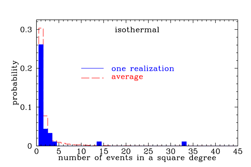
Figure 4: The probability of finding a certain number of events in a one square degree area of the sky

In Fig. 4 we present a histogram showing the number of occurrences of single and multiple events in arrival directions within a square degree. We generated many realizations of the expected subclump distribution, and calculated the flux from the subclumps that would result in about 100 detected events. We see that the average probabilities are quite reasonable, with most events in square degree areas with only one event, and a few pairs and triplets of events. However if we examine individual realizations containing about 100 events, we see that there is a large probability of a large number of events from single nearby subclumps. For instance, in the single realizations shown in Fig. 4, the isothermal subclumps result in a square degree bin with 14 events and a square degree bin with 33 events. If more than 100 events are observed with full sky coverage, the signature of subclumps will be unmistakable.

5 Conclusion

The origin of UHE cosmic rays from annihilation (or decay) of wimpzillas has the attractive feature of the simplicity of generating ultrahigh energies: simple conversion of rest mass energy.

UHE cosmic rays from decay of a smooth relic superheavy dark matter population in the halo requires a lifetime of about $10^{20}\,$years or a correspondingly reduced contribution of the superheavy relics to $\Omega_{dark}$.

In this paper we have examined the annihilation scenario: We found that unitarity limits very likely exclude an appreciable contribution to UHE cosmic rays from standard particle annihilation in the smooth halo component, but monopolonium decay is a possible counterexample to this conclusion.

We also found that annihilation of wimpzilla particles in sub-galactic clumps does not necessarily violate low-$l$ unitarity limits. Like the decay of wimpzillas of lifetime $\tau\sim 10^{10}\,$years, this would also imply $\Omega_{\mathrm{{\sc wimpzilla}}}\ll\Omega_{dark}$.

The annihilation proposal results in several striking predictions. While not discussed in this paper, the annihilation scenario suggests that the bulk of the UHE events are photons. This prediction, common to the decay scenario, seems to be already in conflict with a recent analysis of the composition of the old Haverah Park data, which indicate that no more than $55\%$ of events above $4\times 10^{19}$ eV are consistent with being photons [44]. However, this limit is weaker for events with energy above $10^{20}$ eV. Upcoming data with the large statistics of events required to determine the composition beyond any doubt will soon be available and will definitely test the viability of all the top down models of UHECRs.

The true characteristic signature of the annihilation scenario is the expected anisotropy in arrival direction. If the dark matter is smoothly distributed in the galaxy, the galactic center should be prominent. If the dark matter is clumped on sub-galactic scales, then the subclumps should be visible.

Thus, the annihilation scenario can be falsified by complete sky coverage. The Pierre Auger Observatory and future space based experiments, such as EUSO [45] and OWL [46] will be able to see the galactic center, and, by covering the southern sky, should be able to pick out subclumps if they are present.

Acknowledgement:
R.D. thanks Julio Navarro for a conversation on the NFW halo profile. P.B. and E.W.K. would like to thank Keith Ellis for discussion about QCD hadronization. The work of P.B. and E.W.K. was supported in part by NASA (NAG5-7092). The work of R.D. was supported in part by NSERC Canada.

References

- [1] Y. Mellier, F. Bernardeau, L. van Waerbeke, in Phase Transitions in Cosmology, edited by H. J. de Vega and N. Sanchez, World Scientific, Singapore 1998, pp. 273–287; E. E. Falco, C. S. Kochanek, J. A. Munoz, Astrophys. J. 494 (1998) 47; A. R. Cooray, J. M. Quashnock, M. C. Miller, Astrophys. J. 511 (1999) 562.
- [2] Y. Sigad, A. Eldar, A. Dekel, M. A. Strauss, A. Yahil, Astrophys. J. 495 (1998) 516; E. Branchini, I. Zehavi, M. Plionis, A. Dekel, MNRAS 313 (2000) 491.
- [3] S. Dodelson, L. Knox, Phys. Rev. Lett. 84 (2000) 3523; G. Efstathiou, CMB anisotropies and the determination of cosmological parameters, astro-ph/0002249; W. Hu, M. Fukugita, M. Zaldarriaga, M. Tegmark, Astrophys. J. 549 (2001) 669.
- [4] S. Perlmutter et al., Astrophys. J. 517 (1999) 565.
- [5] S. Burles, D. Tytler, Astrophys. J. 499 (1998) 699, Astrophys. J. 507 (1998) 732; S. Burles, K. M. Nollett, M. S. Turner, Big-bang nucleosynthesis predictions for precision cosmology, astro-ph/0010171.
- [6] K. Greisen, Phys. Rev. Lett. 16 (1966) 748; G. T. Zatsepin, V. A. Kuzmin, JETP Lett. 4 (1966) 78.
- [7] T. Stanev, R. Engel, A. Mücke, R. J. Protheroe, J. P. Rachen, Phys. Rev. D 62 (2000) 093005; M. Blanton, P. Blasi, A. Olinto, Astropart. Phys. 15 (2001) 275.
- [8] G. R. Farrar, T. Piran, Phys. Rev. Lett 84 (2000) 689.
- [9] V. Berezinsky, M. Kachelrieß, A. Vilenkin, Phys. Rev. Lett. 79 (1997) 4302.
- [10] V. A. Kuzmin, V. A. Rubakov, Phys. Atom. Nucl. 61 (1998) 1028.
- [11] K. Benakli, J. Ellis, D. V. Nanopoulos, Phys. Rev. D 59 (1999) 047301.
- [12] V. S. Berezinsky, P. Blasi, A. Vilenkin, Phys. Rev. D 58 (1998) 103515.
- [13] D. J. H. Chung, E. W. Kolb, A. Riotto, Phys. Rev. D 59 (1999) 023501.
- [14] D. J. H. Chung, E. W. Kolb, A. Riotto, Phys. Rev. Lett. 81 (1998) 4048.
- [15] D. J. H. Chung, E. W. Kolb, A. Riotto, Phys. Rev. D 60 (1999) 063504.
- [16] E. W. Kolb, D. J. H. Chung, A. Riotto, in Dark Matter in Astrophysics and Particle Physics 1998, edited by H. V. Klapdor-Kleingrothaus and L. Baudis, IoP Publishing, Bristol 1999, pp. 592–611.
- [17] J. D. Barrow, E. J. Copeland, E. W. Kolb, A. R. Liddle, Phys. Rev. D 43 (1991) 977.
- [18] A. Masiero, A. Riotto, Phys. Lett. B 289 (1992) 73.
- [19] E. W. Kolb, A. Riotto, I. I. Tkachev, Phys. Lett. B 423 (1998) 348.
- [20] D. J. H. Chung, Classical inflaton field induced creation of superheavy dark matter, hep-ph/9809489.
- [21] D. J. H. Chung, E. W. Kolb, A. Riotto, I. I. Tkachev, Phys. Rev. D 62 (2000) 043508.
- [22] G. F. Giudice, M. Peloso, A. Riotto, I. Tkachev, JHEP 9908 (1999) 014.
- [23] V. Kuzmin, I. Tkachev, JETP Lett. 68 (1998) 271, Phys. Rev. D 59 (1999) 123006, Phys. Rep. 320 (1999) 199.
- [24] D. J. H. Chung, P. Crotty, E. W. Kolb, A. Riotto, Phys. Rev. D 64 (2001) 043503.
- [25] R. Dick, Gen. Rel. Grav. 30 (1998) 435.
- [26] R. Dick, Fortschr. Phys. 45 (1997) 537.
- [27] J. L. Crooks, J. O. Dunn, P. H. Frampton, Astrophys. J. 546 (2001) L1.
- [28] J. F. Navarro, C. S. Frenk, S. D. M. White, MNRAS 275 (1995) 720, Astrophys. J. 462 (1996) 563.
- [29] J. F. Navarro, private communication.
- [30] W. Dehnen, J. Binney, MNRAS 294 (1998) 429.
- [31] P. Bhattacharjee, G. Sigl, Phys. Rep. 327 (2000) 109.
- [32] M. Birkel, S. Sarkar, Astropart. Phys. 9 (1998) 297.
- [33] Z. Fodor, S. D. Katz, Phys. Rev. Lett. 86 (2001) 3224.
- [34] Yu. L. Dokshitzer, V. A. Khoze, A. H. Mueller, S. I. Troyan, Basics of Perturbative QCD, Editions Frontières, Gif-sur-Yvette 1991.
- [35] S. Weinberg, The Quantum Theory of Fields Vol. 1, Sec. 3.7, Cambridge University Press, Cambridge 1995.
- [36] K. Griest, M. Kamionkowski, Phys. Rev. Lett. 64 (1990) 615.
- [37] L. Hui, Phys. Rev. Lett. 86 (2001) 3467.
- [38] J. P. Preskill, Phys. Rev. Lett. 43 (1979) 1365.
- [39] C. T. Hill, Nucl. Phys. B 224 (1983) 469.
- [40] E. N. Parker, Astrophys. J. 160 (1970) 383.
- [41] J. J. Blanco-Pillado, K. D. Olum, Phys. Rev. D 60 (1999) 083001.
- [42] V. S. Berezinsky, A. V. Gurevich, K. P. Zybin, Phys. Lett. B 294 (1992) 221.
- [43] V. Berezinsky, A. Bottino, G. Mignola, Phys. Lett. B 391 (1997) 355.
- [44] M. Ave, J. A. Hinton, R. A. Vazquez, A. A. Watson, E. Zas, Phys. Rev. Lett. 85 (2000) 2244.
- [45] See http://www.ifcai.pa.cnr.it/EUSO/
- [46] R. E. Streitmatter, Proceedings of the Workshop on Observing Giant Cosmic Air Showers from eV Particles from Space, eds. Krizmanic, J. F., Ormes, J. F., and Streitmatter, R. E. (AIP Conference Proceedings 433, 1997).