Topics in Basic Maser Theory

Abstract

This review covers some of the developments in basic theory of astronomical masers over the past ten years. Topics included are the effects of three dimensional geometry and polarization, with special emphasis on the differences between maser and non-maser radiation.

Physics & Astronomy Department, University of Kentucky, Lexington, KY 40506, USA; moshe@pa.uky.edu

1. Maser Absorption Coefficient in Three Dimensions

The absorption coefficient $\kappa$ describes the coupling between particles and radiation and serves as the foundation of maser theory. The appropriate expression, taking proper care of the Doppler matching between particles with thermal velocity distribution and photons with a given wave vector k (aligned with the $z$-axis) and frequency $\nu$, was developed by Litvak (1973). It can be written as

$$\hbox{$\kappa$}({\bf k})={c\over\nu_{0}}\int\!\!{\hbox{$\kappa$}_{0}(\hbox{${\bf v}_{\rm k}$})\over 1+I(\hbox{${\bf v}_{\rm k}$})/\hbox{$J_{s}$}}\ dv_{x}dv_{y}\,,$$ (1)

where

$$\hbox{${\bf v}_{\rm k}$}=(v_{x},v_{y},v_{z}=c[\nu-\nu_{0}]/\nu_{0}),\qquad I(\hbox{${\bf v}_{\rm k}$})={1\over 4\pi}\int I(\bf k^{\prime})\delta(\nu^{\prime}-\nu_{0}+\hbox{${\bf v}_{\rm k}$}\cdot{\bf k^{\prime}})d^{3}{\bf k^{\prime}}.$$

Here $I(\bf k)$ is the intensity for wave vector k, $J_{s}$ is the saturation intensity and $\hbox{$\kappa$}_{0}(\bf v)$ is the unsaturated absorption coefficient (proportional to the density of particles with thermal velocity v). Unfortunately, this expression was soon ignored and largely forgotten (except for a couple of papers by Bettwieser & Kegel 1974 and Bettwieser 1976) because shortly thereafter Goldreich & Kwan (1974) introduced the much simpler expression

$$\hbox{$\kappa$}_{\nu}={\hbox{$\kappa$}_{0\nu}\over 1+J_{\nu}/\hbox{$J_{s}$}}\,,$$ (2)

where

$$\hbox{$\kappa$}_{0\nu}={c\over\nu_{0}}\int\!\!\hbox{$\kappa$}_{0}(\hbox{${\bf v}_{\rm k}$})\ dv_{x}dv_{y}\,,\qquad J_{\nu}=\int I_{\nu}{d\Omega\over 4\pi}\,.$$

This expression gives the correct result for linear masers, where photon and particle motions are aligned, and because maser radiation is tightly beamed, Goldreich & Kwan reasoned that it should be adequate for all masers. It became the standard for all subsequent theory, including 3D geometries, even though it was not derived from the proper equation 1. It took many years until Neufeld (1992) recognized the internal inconsistency in this approach: in deriving the standard expression (2) the maser beaming angle is assumed to vanish, yet this very expression is used to solve the maser structure in any given geometry and derive the beaming angle for that geometry.

Fortunately, the standard expression proved to be mostly adequate. Since maser radiation is tightly beamed, equation 1 can be handled with the aid of a series expansion in the beam width and the leading term in such a series reproduces the standard expression 2 (Elitzur 1994). The standard theory provides the correct description of three dimensional masers and its results remain intact but only within the frequency core $|x|\mathrel{\hbox{\hbox to0.0pt{\hbox{\lower 4.0pt\hbox{$\sim$}}\hss}\hbox{$<$}}}\hbox{$x_{s}$}\hbox{$\Delta\nu_{D}$}$, where $\Delta\nu_{D}$ is the Doppler width, $x=(\nu-\nu_{0})/\hbox{$\Delta\nu_{D}$}$ and $x_{s}$ is a dimensionless parameter. For typical pumping schemes $x_{s}$ is $\sim$ 2 in spherical masers, $\sim$ 2.5–3 in disk masers and $\sim$ 3–5 in cylindrical masers. For frequencies outside this core region, interaction with core rays that are slightly slanted to the direction of propagation suppresses photon production. Observed maser radiation is effectively confined to the core region, frequencies in the suppressed domain are essentially unobservable. In practice, suppression only affects extreme maser outbursts. Their profiles change in such a way that when fitted with a Gaussian they mimic line narrowing in proportion to $(\ln F_{0})^{-1/2}$, where $F_{0}$ is the flux at line center, in contrast with the standard theory where such behavior is confined to unsaturated amplification. Such an inverse correlation between intensity and linewidth has been detected in a number of H₂O maser flares in star-forming regions (e.g. Mattila et al 1985, Rowland and Cohen 1986, Boboltz et al 1993, Liljestrom 1993).

1.1. Linewidths in 3D Masers

Maser radiation is tightly beamed, therefore the intensity $I_{\nu}$, angle-averaged intensity $J_{\nu}$ and flux $F_{\nu}\ (=\int\mu I_{\nu}d\Omega)$ are related via

$$F_{\nu}=4\pi J_{\nu}=I_{\nu}\hbox{$\Omega_{b}$}$$ (3)

where $\Omega_{b}$ is the beaming solid angle. Saturated masers display two types of beaming (Elitzur, Hollenbach & McKee 1992). In matter-bounded masers, whose prototype is the filamentary maser, the beaming angle is controlled by the matter distribution and the maser observed size is equal to its physical size. The beaming angles of such masers are frequency independent, therefore the frequency profiles are the same for $F_{\nu}$ and $I_{\nu}$. In amplification-bounded masers, whose prototype is the spherical maser, the beaming angle is controlled by the amplification process and the observed size is significantly smaller than the physical size. Because the amplification is strongest at line center the beaming is tightest there; the beaming angle increases with frequency shift from line center and the spectral shapes of $F_{\nu}$ and $I_{\nu}$ are different from each other.

With the standard expression for the absorption coefficient (2), it is easy to show that the flux of a saturated maser increases with length $\ell$ according to $F_{\nu}\propto\hbox{$\kappa$}_{0\nu}\hbox{$J_{s}$}\ell$ independent of the geometry (Elitzur 1990). Even with the full, proper equation 1, the standard theory remains applicable at the core of the line so this result too is valid there. Therefore, in any saturated maser the frequency profile of the flux always obeys $F_{\nu}\propto\hbox{$\kappa$}_{0\nu}\propto\exp(-x^{2})$, i.e., the flux spectral shape displays the full Doppler width $\Delta\nu_{D}$. On the other hand, the intensity obeys $I_{\nu}\propto F_{\nu}/\hbox{$\Omega_{b}$}$, therefore its spectral pprofile will reflect also the frequency dependence of $\Omega_{b}$. The result is $I_{\nu}\propto\hbox{$\kappa$}_{0\nu}^{\alpha}\propto\exp(-\alpha x^{2})$ where $\alpha$ is the dimensionality of the geometry; $\alpha$ is 1 for linear or filamentary masers, 2 for planar masers such as disks and 3 for fully 3D structures such as spheres. The width of the brightness spectral shape is thus

$$\Delta\nu={\hbox{$\Delta\nu_{D}$}\over\sqrt{\alpha}}.$$ (4)

In particular, the intensity linewidth of a saturated planar maser (the most likely geometry for shock induced masers) is 40% smaller than the Doppler width.

2. Polarization

Thermal radiation is generated in spontaneous decays, maser radiation in stimulated emission. This fundamental difference has profound implications, especially for polarization.

The stimulated emission process is the inverse of radiation absorption. Absorption is a purely classical process, therefore the same applies also to stimulated emission. Since line radiation involves discrete energy states, the particle properties must be described with quantum mechanics. But the radiation wavelength is many orders of magnitude larger than particle dimensions so there is no need to quantize also the radiation field. The interaction of matter with maser radiation is adequately described with a hybrid, semi-classical approach (Litvak 1970; Goldreich, Keeley, & Kwan 1973, GKK hereafter): The radiation field is described by standard classical electromagnetic waves. The energy levels are eigenstates of the system Hamiltonian, treated by quantum theory. Interaction with the radiation field, treated as a perturbation, causes transitions between the energy levels. The transition rates for both absorption and stimulated emission are obtained from the product of the (quantum) matrix element of the transition dipole moment with the (classical) intensity of the radiation field. Since this is a complete description, not merely a classical analog, an important consequence is that there are no properties of the radiation generated in stimulated emission that are peculiar to the quantum theory; we must be able to fully deduce all of them from purely classical concepts as applied to propagating electromagnetic waves.

In contrast, spontaneous emission is a purely quantum process. It has no classical analog since the initial state is devoid of radiation and thus cannot interact with any electromagnetic wave. Spontaneous decays do not occur even in standard treatments of quantum theory because the energy levels are stationary states of the system Hamiltonian, completely stable in the absence of external perturbations. This process occurs only when quantization of the electromagnetic field is taken into considerations, and can be interpreted as scattering off vacuum fluctuations. Spontaneous emission can be analyzed only in terms of the photon description of the radiation field.

Induced Photons

When stimulated emission is described in terms of photons, energy and momentum conservation imply that the induced photon has the same frequency and direction as the parent photon. However, contrary to some widespread misconceptions, the induced photon does not have the same

1. Phase: The argument of the oscillatory behavior of any wave is its phase $\phi=\phi_{0}+\omega t-\,{\bf k\!\cdot\!r}$, where $\omega$ is the angular frequency and k is the wave vector. An electromagnetic wave has a phase, a photon does not. The uncertainty principle leads to the relation $\Delta n\Delta\phi\geq 1$ between phase and photon number. The phase of a state with a well-defined number of photons is completely undetermined. Phases are meaningless when dealing with photon numbers, in particular they are irrelevant in spontaneous emission.

2. Polarization: The induced photon polarization is not necessarily equal to that of the parent photon. Instead, it is determined by the change in magnetic quantum number $m$ of the interacting particle. $\Delta m$ = 0 transitions couple to photons linearly polarized along the quantization axis, $\hbox{$\Delta m$}=\pm 1$ transitions couple to photons that are right- and left-circularly polarized in the plane perpendicular to the quantization axis. Consider the interaction of a linearly polarized photon with particles in the upper level of a spin $1\to 0$ transition. When the interacting particle is in the $m=0$ state it executes a $\Delta m$ = 0 transition and the induced photon, too, is linearly polarized. But this is not the case when the particle is in one of the $|m|$ = 1 states. The linearly polarized photon, which can also be described as a coherent mixture of two circularly polarized photons, will now induce a $|\hbox{$\Delta m$}|=1$ transition and the induced photon is circularly polarized. Induced emission preserves polarization only when the magnetic transitions do not overlap.

2.1. Polarization in Spontaneous Decays

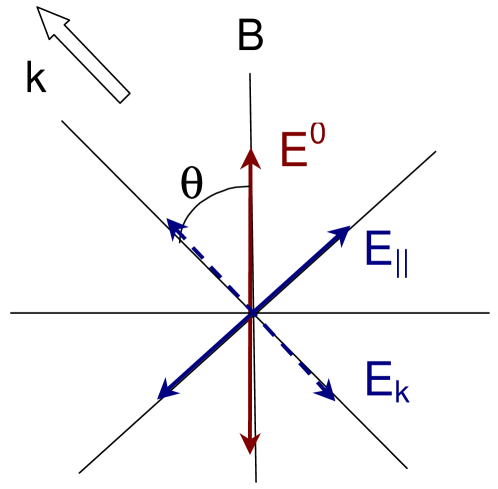
Figure 1.: Polarization in $\Delta m$ = 0 spontaneous emission.

From Maxwell’s equations, the electric field of an electromagnetic wave is always perpendicular to the propagation direction. This seemingly simple transverse condition is a rather peculiar constraint, hard to reconcile with the properties of the quantized particles that emit line radiation. Figure 1 shows the geometry for a $\Delta m$ = 0 spontaneous decay. The quantization axis is denoted by $B$. The electric field generated in the transition, with an amplitude $E^{0}$, is always parallel to this axis. The photons propagate in the direction marked by the double arrow at an angle $\theta$ from $B$, the corresponding axis is denoted $k$. The component of the electric field along the axis parallel to the projection of $B$ on the plane of the sky is $\hbox{$E_{\|}$}=E^{0}\sin\theta$. What about the component along the direction of propagation, $E_{k}$? Is it $E^{0}\cos\theta$ as the geometry dictates? Or is it 0 as required by the transverse condition? How can we reconcile these conflicting results? The answer is that we cannot as long as we apply classical reasoning. The resolution of this conflict is rooted in the quantum nature of spontaneous emission, which has no classical analog. Because of the uncertainty principle, only one component of any vector can be determined whenever the magnitude of that vector is known, the other two remain undetermined; recall the properties of angular momentum. The longitudinal component can be ignored in spontaneous emission—quantum mechanics can be counted on to take care of the transverse condition $E_{k}=0$ and we can proceed directly to calculate the polarization. Denote by $I^{0}$ the intensity associated with the amplitude $E^{0}$ ($I^{0}\propto|E^{0}|^{2}$). Then the intensities measured by a linear antenna oriented parallel and perpendicular to the $B$-axis are, respectively, $\hbox{$T_{\|}$}=I^{0}\sin^{2}\theta$ and $\hbox{$T_{\bot}$}=0$. Therefore, the Stokes parameters of $\Delta m$ = 0 spontaneous emission are $I=\hbox{$T_{\|}$}+\hbox{$T_{\bot}$}=I^{0}\sin^{2}\theta$ and $Q=\hbox{$T_{\|}$}-\hbox{$T_{\bot}$}=I$, recovering the standard result of full linear polarization.

2.2. Fully Resolved Zeeman Pattern; $\hbox{$\nu_{B}$}\gg\hbox{$\Delta\nu_{D}$}$

When the magnetic field is sufficiently strong that the Zeeman shift $\nu_{B}$ exceeds the linewidth $\Delta\nu_{D}$, radiation is produced in pure $\Delta m$ transitions centered on the appropriate Zeeman frequencies. For the $\Delta m$ = 0 transition we have just derived the polarization and it is straightforward to repeat these calculations for $\hbox{$\Delta m$}=\pm 1$ spontaneous emission. The results are summarized in table 1 for the classical Zeeman pattern. In that case there are three spectral lines centered on $\nu_{0}+\hbox{$\nu_{B}$}\hbox{$\Delta m$}$ ($\Delta m$ = 0, $\pm 1$), where $\nu_{0}$ is the line frequency in the absence of a magnetic field, with $I^{0}(\nu)=I^{+}(\nu+\hbox{$\nu_{B}$})=I^{-}(\nu-\hbox{$\nu_{B}$})$. Quantities listed in the first column are obtained for each transition from the product of the intensity heading the transition column with the appropriate trigonometric factor. The intensities that would be measured with right- and left-circular instrumental response are listed as $T_{r,\,l}$ and $V=T_{r}-T_{l}$. The parameter $U$ vanishes for all transitions with this choice of axes.

	$\sigma^{+}$	$\pi$	$\sigma^{-}$
	$\hbox{$\,{}^{1}\!/_{4}$}I^{+}$	$\hbox{$\,{}^{1}\!/_{2}$}I^{0}$	$\hbox{$\,{}^{1}\!/_{4}$}I^{-}$
$T_{\|}$	$2\cos^{2}\theta$	$2\sin^{2}\theta$	$2\cos^{2}\theta$
$T_{\bot}$	2	0	2
$T_{r}$	$(1+\cos\theta)^{2}$	$\sin^{2}\theta$	$(1-\cos\theta)^{2}$
$T_{l}$	$(1-\cos\theta)^{2}$	$\sin^{2}\theta$	$(1+\cos\theta)^{2}$
$I$	$2(1+\cos^{2}\theta)$	$2\sin^{2}\theta$	$2(1+\cos^{2}\theta)$
$Q$	$-2\sin^{2}\theta$	$2\sin^{2}\theta$	$-2\sin^{2}\theta$
$V$	$4\cos\theta$	0	$-4\cos\theta$

Table 1.: Polarizations for fully resolved Zeeman pattern, $\nu_{B}\gg\hbox{$\Delta\nu_{D}$}$

The results display the standard polarization properties of thermal radiation of fully resolved Zeeman components. And because each component can be considered an independent, isolated radiative transition that couples to a single sense of polarization, these results apply also to maser radiation even though they were derived for spontaneous emission. Indeed, these are the maser polarization properties derived by GKK, although from an entirely different approach. Thermal and maser polarizations are the same when the Zeeman pattern is fully resolved. The only difference between the two cases is the disparity between the $\pi$ and $\sigma$ maser intensities, reflecting their different growth rates (Elitzur 1996). This disparity predicts a preponderance of $\sigma$-components. However, the evidence is mounting that individual $\pi$-components are in fact never observed, a puzzle that currently has no explanation.

2.3. Overlapping Zeeman Components; $\hbox{$\nu_{B}$}\ll\hbox{$\Delta\nu_{D}$}$

The thermal and maser cases diverge now because the stimulated emission mixes the polarization components. Thermal emission is produced in spontaneous decays and must be considered in the photon picture; only intensities, i.e., photon numbers, are relevant. Maser radiation is generated in stimulated emission and its properties must be understood in terms of classical waves interacting with particles in quantized energy levels; both amplitudes and phases count.

Thermal Radiation

The various $\Delta m$ transitions produce spectral components with equal intensities but centered on frequencies slightly shifted from each other. The intensity $I^{0}$ of the $\Delta m$ = 0 component is an even function of $x$, centered on $x=0$. Introduce $\hbox{$x_{B}$}=\nu_{B}/\hbox{$\Delta\nu_{D}$}\ll 1$, then $I^{\pm}(x\pm\hbox{$x_{B}$})=I^{0}(x)$. The three components are produced independent of each other and the overall radiation field is an incoherent superposition of them. Within each component the transverse condition is obeyed independently and the photons are polarized as described in table 1. Adding up the Stokes parameters at every frequency across the line yields

$$I = I^{0}+I^{+}+I^{-}=2I^{0}$$

$$Q = Q^{0}+Q^{+}+Q^{-}=\left[I^{0}-\hbox{$\,{}^{1}\!/_{2}$}(I^{+}+I^{-})\right]\sin^{2}\theta=-{d^{2}I\over dx^{2}}\,(\hbox{$x_{B}$}\sin\theta)^{2}$$

$$V = V^{0}+V^{+}+V^{-}=(I^{+}-I^{-})\cos\theta={dI\over dx}\,\hbox{$x_{B}$}\cos\theta$$ (5)

The final expression in each case is the leading order result from a series expansion in $x_{B}$ of $I^{\pm}(x)$ around $I^{0}(x)$. The overall radiation field is polarized because it is the superposition of three polarized different intensities—because of the Zeeman shifts the intensities are slightly different at every given frequency. These differences are controlled by the parameter $x_{B}$, and so is the polarization. When $\hbox{$x_{B}$}\ \to 0$, the polarization disappears.

Overlapping Electromagnetic Waves

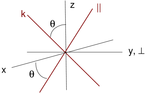
Figure 2.: Geometry of the wave and quantization frames.

At a given frequency and wave vector, each $\Delta m$ (= $0,\pm 1$) transition produces an electric vector with magnitude

$$E^{\Delta m}=|E^{\Delta m}|\,e^{i({\bf k\cdot r}-\omega t+\phi_{\Delta m})},$$ (6)

where the initial phase $\phi_{\Delta m}$ is random. The overall electric vector is ${\bf E}=\sum{{\bf E}^{\Delta m}}$ and must obey the transverse condition ${\bf E\cdot k}=0$. The geometrical setup is shown in figure 2. Particle quantization is defined with respect to the $x$-$y$-$z$ coordinate frame, with $z$ the quantization axis. In this frame, each component of E is uniquely associated with a specific $\Delta m$: the $z$-component couples only to $\Delta m$ = 0, so that $E^{0}=E_{z}$, the $x$- and $y$-components couple only to $\hbox{$\Delta m$}=\pm 1$, i.e., $E^{\pm}=2^{-1/2}(E_{x}\pm iE_{y})$. The wave propagation is along the $k$-axis, rotated by an angle $\theta$ from the quantization axis in the $x$-$z$ plane. Since the electric field is a proper vector, it can be decomposed in this frame too using straightforward, standard geometry. The transverse condition states that $E_{k}=0$ irrespective of the direction of propagation, and now we cannot rely on quantum considerations; this condition must be obeyed as a geometrical constraint on the three vector components of E (eq. 6). Given the amplitudes $|E^{\Delta m}|$, the condition $E_{k}=0$ becomes a relation among the phases $\phi_{\Delta m}$. For example, when $|E^{0}|=|E^{+}|=|E^{-}|$ the relation is

Figure 3.: 90^∘ flip of SiO linear polarization in TX Cam (Kemball & Diamond 1997)

$$\phi_{+}=-\phi_{-}\,,\qquad\phi\equiv|\phi_{\pm}|=\arccos\left(2^{-1/2}\cot\theta\right),$$ (7)

where the meaningless overall phase is set through $\phi_{0}=0$ (Elitzur 1991); one $\sigma$-component leads the $\pi$-component by the phase difference $\phi$ and the other must trail by the exact same amount. Only waves launched with these phase relations produce superpositions that are purely transverse so that they can be amplified by propagation in the inverted medium. The transverse components of these propagating waves are linearly polarized according to

$$q={Q\over I}=-1+{2\over 3\sin^{2}\theta}\ .$$ (8)

Whereas the thermal polarization arises from the superposition of different intensities, this one involves equal intensities but well defined phase relations among the amplitudes. The polarization arises because the independent constraints imposed by the particle interactions and the transverse condition must be reconciled simultaneously. Particle interactions (i.e., maser pumping) produce three independent fields corresponding to $\Delta m$ = $0,\pm 1$. The transverse condition dictates that only two independent fields propagate in any given direction, the longitudinal combination of the original fields must vanish. The resulting phase relation, and polarization, reflect the correlation that must exist to eliminate the longitudinal component of E. The linear polarization in eq. 8 depends only on propagation angle, it is entirely independent of $x_{B}$. Indeed, the only assumption in its derivation was the existence of a quantization axis in the source—the physical process behind this axis was never specified, in principle it need not be a magnetic field.

Equation 8 is immediately recognized as the polarization solution derived by GKK from an entirely different approach. Their assumption of equal pump rates for the different $m$-states is reflected in the equal $|E^{\Delta m}|$ taken here. The polarization becomes unphysical ($q>1$) for $\sin^{2}\theta<\hbox{$\,{}^{1}\!/_{3}$}$. Only unpolarized maser radiation can propagate there since the interference dictated by the transverse condition cannot be obeyed for equal $|E^{\Delta m}|$. The polarization changes sign at $\sin^{2}\theta=\hbox{$\,{}^{2}\!/_{3}$}$, where it vanishes. At smaller (larger) angles $q$ is positive (negative), corresponding to polarization along (perpendicular to) the quantization axis. The transition between positive and negative $q$ corresponds to a 90^∘ flip in the polarization direction. Such flips are commonly observed in SiO masers; an example is shown in figure 3. A natural explanation is a slight change in direction of the magnetic field, straddling the two sides of the transition angle $\theta=55\hbox{${}^{\circ}$}$.

It is important to note that the linear polarization will usually not exceed 33% because only the limited range $35\hbox{${}^{\circ}$}\leq\theta\leq 45\hbox{${}^{\circ}$}$ gives $|q|>\hbox{$\,{}^{1}\!/_{3}$}$. Propagation at $\theta>45\hbox{${}^{\circ}$}$ gives only $|q|\leq\hbox{$\,{}^{1}\!/_{3}$}$—along the field when $45\hbox{${}^{\circ}$}\leq\theta<55\hbox{${}^{\circ}$}$ and orthogonal to it when $\theta>55\hbox{${}^{\circ}$}$. The direction of the magnetic axis is generally not known a-priori. It can be determined with certainty only when the linear polarization exceeds 33%, in which case the field projection on the plane of the sky must be parallel to the polarization.

Maser Polarization

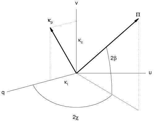
Figure 4.: The polarization vector ${\bf\Pi}$ and the vector $\kappa_{p}$ that controls its radiative transfer in the space defined by the normalized Stokes parameters $q=Q/I$, $u=U/I$ and $v=V/I$.

The preceding discussion provides a geometric derivation of the structure of polarization consistent with the fundamental physical processes that generate maser radiation. Equation 8 lists the only polarization consistent with the constraints that govern an interacting mixture of quantized particles and classical electromagnetic waves that have equal amplitudes in the quantization frame. In actuality, we cannot know these amplitudes beforehand and must derive them from a complete solution for the level populations coupled to the polarized radiation. The radiative transfer equation involves a matrix in the space of four Stokes parameter, presenting a rather complex problem. An elegant geometrical interpretation was derived by Litvak (1975). The polarization structure of any electromagnetic wave is defined by the 3-vector of its normalized Stokes parameters $\hbox{${\bf\Pi}$}=(q,u,v)$ (figure 4). The off-diagonal elements of the radiative transfer matrix are $\hbox{$\kappa_{l}$}\propto\hbox{$\,{}^{1}\!/_{2}$}(n_{1}^{+}+n_{1}^{-})-n_{1}^{0}$ and $\hbox{$\kappa_{c}$}\propto n_{1}^{+}-n_{1}^{-}$, where $n_{1}^{m}$ is the population of the magnetic $m$-state of the upper level. These elements can be combined to form another 3-vector $\mbox{\boldmath$\kappa_{p}$}=(\hbox{$\kappa_{l}$},0,\hbox{$\kappa_{c}$})$, then

$${d\hbox{${\bf\Pi}$}\over d\ell}=\left[\hbox{${\bf\Pi}$}\hbox{$\times$}\mbox{\boldmath$\kappa_{p}$}\right]\hbox{$\times$}\hbox{${\bf\Pi}$}\,.$$ (9)

The effect of radiative transfer is to rotate the polarization vector of each individual electromagnetic wave at the rotation velocity ${\bf\Pi}$$\times$$\kappa_{p}$; this velocity is different for different waves and changes as ${\bf\Pi}$ is rotating. Since waves are launched with arbitrary initial polarizations that subsequently rotate at different rates, the radiation field can be expected to remain unpolarized unless there is a stationary configuration whose polarization vector does not rotate. When such a configuration exists, the polarization vectors are locked once they enter it and that becomes the polarization of the overall radiation field.

Stationary polarization obviously occurs when $\hbox{${\bf\Pi}$}\ \|\ \mbox{\boldmath$\kappa_{p}$}$ . However, since the level populations are affected by the interaction with the maser radiation, $\kappa_{p}$ itself varies and is affected by ${\bf\Pi}$, therefore one must find a formalism to identify the stationary polarizations. It is straightforward to show that they are the eigenvectors of the radiative transfer matrix (Elitzur 1996). Two types of solutions exist for masers in a magnetic field. One type corresponds to the $\hbox{$x_{B}$}\gg 1$ case, the other to $\hbox{$x_{B}$}\ll 1$. The solution for the latter reproduces the GKK linear polarization (8) accompanied by the circular polarization

$$v={16x\hbox{$x_{B}$}\over 3\cos\theta}\,.$$ (10)

This polarization arises when the populations of the magnetic sub-states of each level become equal to each other as a result of maser radiative interaction, requiring a unique cooperation between the particles and the radiation that they amplify. It is reached only in masers with $\hbox{$J_{s}$}\gg S$, where $S$ is the source function, after the radiation has grown so that $J/\hbox{$J_{s}$}\mathrel{\hbox{\hbox to0.0pt{\hbox{\lower 4.0pt\hbox{$\sim$}}\hss}\hbox{$>$}}}\hbox{$x_{B}$}$. The condition $q^{2}+v^{2}\leq 1$ constrains the propagation directions for polarized maser radiation.

When the transition frequency varies, the Doppler width $\Delta\nu_{D}$ varies proportionately while the Zeeman splitting $\nu_{B}$ is unaffected. Therefore $x_{B}$ is inversely proportional to frequency, and the circular polarization decreases with the transition frequency when all other properties remain fixed. McIntosh, Predmore & Patel (1994) find that SiO circular polarization indeed decreases when the rotation quantum number, and with it transition frequency, increases. The linear polarization displays the opposite trend, increasing with rotation quantum number (McIntosh & Predmore 1993). Since the solution linear polarization is independent of transition wavelength, this is the expected behavior in the presence of Faraday depolarization, which is proportional to $\lambda^{2}$. The low rotation states are more severely affected because of their longer wavelengths and the linear polarization can be expected to decrease toward lower angular momenta, as observed. Although detailed calculations of Faraday rotation have yet to be performed for $\hbox{$x_{B}$}\ll 1$, McIntosh & Predmore find this to be the most plausible explanation of the data.

2.4. Limitations and Outstanding Issues

The theory presented here was developed for an idealized maser. The results depend in a crucial manner on the assumption of a constant direction for the quantization axis. They provide the maximal polarization that can be produced in a source that maintains a uniform direction for the magnetic field. Any curvature in the field lines along the propagation direction results in $\theta$ variations that destroy the phase coherence between the $\pi$- and $\sigma$-components, reducing the degree of polarization. In particular, Alfven waves introduce ripples in the field lines that destroy the polarization whenever the Alfven wavelength is shorter than the amplification length. Similarly, velocity blending will reduce circular polarization (Sarma, Troland & Romney, 2001) and linear polarization may also be reduced by Faraday rotation. As a result, the information that can be extracted from polarization alone is limited because the same polarization can be produced in a number of different ways. For example, a certain linear polarization can be attributed either to the maximal polarization at an appropriate angle $\theta$ or to a higher degree of polarization that was degraded either by curvature in the field lines or by Faraday depolarization.

Another fundamental assumption is that the only degeneracy of the maser levels involves their magnetic sub-states. When any of the levels includes additional degeneracy, so that magnetic sub-states of different levels overlap, the tight constraints responsible for the stationary solutions no longer apply and the polarization can be expected to disappear. Indeed, the energy levels of both H₂O and methanol involve hyperfine degeneracy and both masers are generally only weakly polarized. Exceptions do exist, though, and H₂O masers sometime display high polarization, notably during outbursts such as in Orion (e.g., Abraham & Vilas Boas 1994). This may involve the excitation of a single hyperfine component, in which case the general solutions derived here are applicable.

Incompleteness

The theory presented here is incomplete. The radiation field is an ensemble of waves launched with random polarizations. Subsequent maser amplification through particle interactions is accompanied by rotation of each polarization vector, and we have identified the stationary modes that do not rotate. However, we have not shown how the radiation field actually evolves into this solution, and this is considerably more difficult. Indeed, it is always simpler to identify the stationary limit of a statistical distribution than to demonstrate how this limit is actually attained. Demonstrations of the approach to Maxwellian of a particle velocity distribution or to Planckian of a photon distribution are considerably more difficult than the derivation of either functional form. The evolution of such ensembles requires numerical simulations of the type frequently performed in studies of plasma and laboratory lasers. This approach can be avoided in the analysis of thermal radiation polarization, where phases are meaningless. But the essence of the maser polarization solution is specific phase relations among waves generated in different $\Delta m$ transitions, and those cannot be captured by standard radiative transfer techniques—the very derivation of the radiative transfer equation from Maxwell’s equations is predicated on the assumption of random phases for different waves (cf Litvak 1970, GKK). A full simulation of the ensemble evolution of interacting particles and waves is the only way to study maser polarization growth. Such simulations have not yet been attempted for astronomical maser radiation. In addition to their inherent significance for demonstrating the approach to stationary polarization, these simulations are essential for a complete analysis of Faraday depolarization when $\hbox{$\nu_{B}$}\ll\hbox{$\Delta\nu_{D}$}$.

Acknowledgments.

The support of an IAU travel grant and NSF grant AST-9819368 is gratefully acknowledged.

References

- 1 Abraham, Z. & Vilas Boas, J.W.S. 1994, A&A 290, 956
- 2 Bettwieser, E. 1976, A&A 50, 231
- 3 Bettwieser, E. V. & Kegel, W. H. 1974, A&A 37, 291
- 4 Boboltz, D., et al 1993, in Astrophysical Masers, eds. G. Nedoluha and A. W. Clegg (Berlin: Springer Verlag), p. 275
- 5 Elitzur, M. 1990, ApJ 363, 638
- 6 Elitzur, M. 1991, ApJ 370, 407
- 7 Elitzur, M. 1994, ApJ 422, 751
- 8 Elitzur, M. 1996, ApJ 457, 415
- 9 Elitzur, M., Hollenbach, D.J. & McKee, C.F. 1992, ApJ 394, 221
- 10 Goldreich, P., Keeley, D.A. & Kwan, J.Y. 1973, ApJ, 179 111 (GKK)
- 11 Goldreich, P. & Kwan, J. 1974, ApJ 190, 27
- 12 Kemball, A.J., & Diamond, P.J. 1997, ApJ, 481, L111
- 13 Liljestrom, T. 1993, in Astrophysical Masers, eds. G. Nedoluha and A. W. Clegg (Berlin: Springer Verlag), p. 291
- 14 Litvak, M.M. 1970, Phys. Rev., A2, 2107
- 15 Litvak, M.M. 1973, ApJ 182, 711.
- 16 Litvak, M.M. 1975, ApJ, 202, 58
- 17 Mattila, K., et al 1985, A&A 145, 192
- 18 McIntosh, G. & Predmore, C. R. 1993, ApJ 404, L71.
- 19 McIntosh, G., Predmore, C. R. & Patel. N. A. 1994, ApJ 428, L29
- 20 Neufeld, D. 1992, ApJ 393, L37
- 21 Rowland, P. R. and Cohen, R. J. 1986, MNRAS 200, 233
- 22 Sarma, A., Troland, T.H. & Romney, J.D. 2001, ApJ Lett, to be published
- 23