Early galaxy evolution from deep wide field star counts

Star counts at high and intermediate galactic latitudes, in the visible and the near infrared, are used to determine the density law and the initial mass function of the thick disc population. The combination of shallow fields dominated by stars at the turnoff with deep fields allows the determination of the thick disc mass function in the mass range 0.2-0.8M_⊙. Star counts are compared with simulations of a synthesis population model. The fit is based on a maximum likelihood criterion. The best fit model gives a scale height of 800 pc, a scale length of 2500 pc and a local density of 10^-3 stars pc^-3 or 7.1 10^-4 M_⊙pc^-3 for Mv $\leq$ 8. The IMF is found to follow a power law dN/dm $\propto$ m^-0.5. This is the first determination of the thick disc mass function.

1 Introduction

Solving the problem of the origin of the thick disc of the Milky Way depends on accurate determination of its present characteristics. Overall analysis of density, kinematics and chemical properties help the understanding of the physical processes involved. A first step was obtained with the finding that the thick disc was probably formed by a merging event on the thin disc early in the early age of the Milky Way (Sommer-Larsen & Antonuccio-Delogu, 1993; Robin et al., 1996). This hypothesis was motivated by the kinematic findings (no gradient, no discontinuity between thin disc and thick disc in rotation and velocity dispersion) and abundances, in particular the [O/Fe] and [Mg/Fe] ratios. These ratios implies a sudden decrease in star formation rate between the thick disc and thin disc formation, lasting for at least 1 Gyr but not more than 3 Gyr (Gratton et al., 2000). More work is required to measure an accurate density law and to obtain a detailed description of the stellar population, such as the initial mass function and age.

The thick disc density law can reasonably be modeled by a double exponential, or a density law close to a sech². Star counts are presently unable to distinguish between these hypotheses. Even the determination of the scale height and the local density causes difficulties due to a slight degeneracy between these two parameters, as shown in various published results. Different analyses have resulted in either high scale height and small local density (for example, Reid & Majewski (1993): 1400 pc and local density of 2% of the disc) or small scale height and higher local density (Robin et al. (1996): 760 pc and density of 5.6%, Buser et al. (1999): 910 pc and 5.9%), with several intermediate results. The number of observed stars is derived by the integral of the density law over the line of sight. For an exponential density law, the mean distance of the stars in a complete sample is roughly twice the scale height. The thick disc dominates star counts at distances between 2 and 5 kpc over the galactic plane. However, photometric counts are not accurate enough to estimate the distances of stars at the turnoff with an accuracy of even a factor of two. Moreover no accurate determination of the local density has ever directly been done, even with Hipparcos, because of the small proportion of the thick disc locally with regard to the thin disc.

The determination of the initial mass function (IMF) of the thick disc is an important issue in the controversy about the universality of the IMF. Scalo (1998) and Kroupa (2001) find that it flattens at masses below 0.5M_⊙, either in our Galaxy or in the LMC. Whereas Scalo points out the difficulty measuring an IMF and argues that the uncertainties on the determination could be of the order of the apparent variations of the IMF, Kroupa analyzes in detail the variations of the IMF slope and concludes that star formation in higher metallicity environments appears to produce relatively more low-mass stars, i.e. a steeper slope at low masses. If confirmed, one should expect the thick disc to have a shallower IMF slope than the thin disc on average.

Until now no direct measurement of the thick disc IMF has been done. All along the main sequence, the thick disc population is easily distinguishable from the disc and the halo using a good temperature indicator like the V-I index, because at a given magnitude below the turnoff of the halo ($\simeq$ V $>$ 17), the blue side is dominated by the halo and the red side by the disc, with the thick disc in between. At high latitudes, thick disc stars become a sizeable population at magnitude about 14-15 in V in wide field star counts when a significant proportion of turnoff stars are detectable on the blue side of the colour distribution. One can reach the peak of the luminosity function (at about M_V=11) at magnitude 21 for stars at 1 kpc. By combining shallow star counts dominated by turnoff stars with deep photometry one should be able to compute the IMF slope on a large mass range, between the turnoff at about m = 0.8 M_⊙and the maximum near m = 0.2 M_⊙.

In this paper we address the problem of the thick disc density law together with its IMF. The two problems cannot be treated separately from star count analysis. We use a large set of stellar samples (described in section 2), in the visible and the near infrared, at shallow and deep magnitudes, to investigate the thick disc luminosity function, the local density and its scale height and scale length. This analysis has been feasible using a coherent model of population synthesis which takes into account the various photometric systems of the data, different basic hypotheses on the parameters to test, and allows us to disentangle the bias effects in star count samples (section 3). A maximum likelihood test is used to estimate the thick disc parameters (section 4). Results are given in section 5 and discussed in section 6.

2 Selected data sets

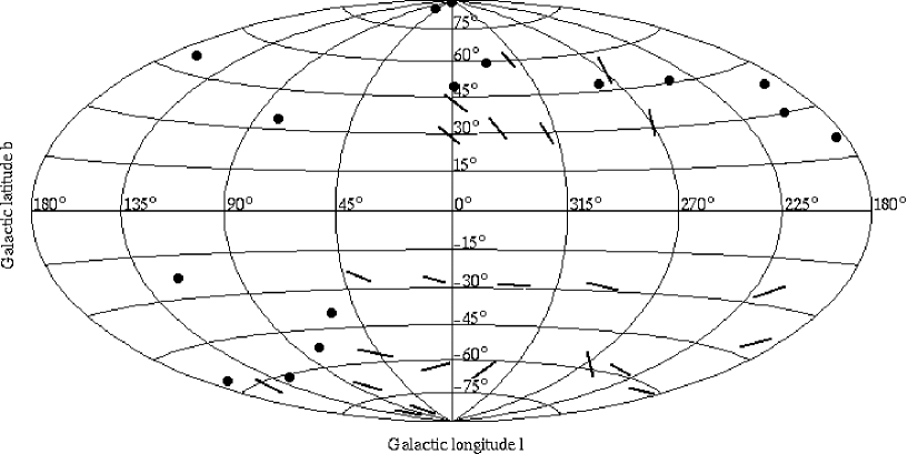
Figure 1: Galactic coordinates of the selected fields. Characteristics of the fields plotted with dots are given in table 1. The lines represent parts of DENIS strips.

Data sets at medium and high galactic latitudes have been selected. They combine shallow and deep star counts, in the visible and the near infrared. The main characteristics of visible data are summarized in table 1. The dots in figure 1 give their distribution in galactic coordinates. The shallow star counts are three wide fields from Ojha et al. (1996, 1999), one field from Chiu (1980) close to the galactic anticentre and one patch from the CNOC2 Field Galaxy Redshift Survey (Yee et al., 2000). The deep fields are one field from Borra & Lepage (1986), one field from Reid & Majewski (1993) close to the North Galactic Pole, six fields from the DMS (Hall et al., 1996; Osmer et al., 1998) used to search for quasars, two fields from Bouvier et al. (1998) dedicated to the study of Pleiades and Praesepe clusters, and another field near the North Galactic Pole (SA57) obtained at the CFHT by Crézé et al. (in preparation). This field is the deepest one. It is complete and free from significant galaxy contamination up to V=24.

We also used near infrared data in I and J bands from the Deep Near Infrared Survey of the Southern Sky: DENIS (Epchtein et al., 1997, 1999) reduced at the Paris Data Analysis Center. DENIS fields, named strips, are 12’ in right ascension and 30^∘ in declination. We have selected 26 strips distributed on the sky at latitudes greater than 30^∘, as shown by the lines in figure 1. At lower latitudes, the disc population becomes dominant compared to the thick disc population. Selected samples are portions of strips over which the density gradient in declination is negligible. They cover 1 to 3 square degrees and are complete up to I=17.5 or I=18, depending on the strip.

The absolute visual magnitude of thick disc stars in the selected samples covers a wide range, from M${}_{V}\simeq$ 4 up to 13. It peaks at M${}_{V}\simeq$ 4-5 in the DENIS fields, M${}_{V}\simeq$ 6-7 in the shallow fields, M${}_{V}\simeq$ 9-10 in the deep fields and M${}_{V}\simeq$ 12 in SA57.

3 The model of population synthesis

We have used a revised version of the Besançon model of population synthesis. Previous versions were described in Bienaymé et al. (1987a, b); Haywood et al. (1997); Robin et al. (2000).

The model is based on a semi-empirical approach, where physical constraints and current knowledge of the formation and evolution scenario of the Galaxy are used as a first approximation for the population synthesis. The model involves 4 populations (disc, thick disc, halo and bulge) each deserving a specific treatment. The bulge population, which is irrelevant for this analysis, will be described elsewhere.

3.1 The disc population

A standard evolution model is used to produce the disc population, based on a set of usual parameters : an initial mass function (IMF), a star formation rate (SFR) and a set of evolutionary tracks (see Haywood et al., 1997, and references therein). The disc population is assumed to evolve over 10 Gyr. A set of IMF slopes and SFRs are tentatively assumed and tested against star counts.

A revised IMF has been used in the present analysis, tuned with the most recent Hipparcos results: the age-velocity dispersion relation is from Gomez et al. (1997), the local luminosity function is from Jahreiss & Wielen (1997) and an IMF power law dN/dm $\propto$ m^-α is adjusted to it, giving a slope $\alpha$ = 1.6 in the low mass range 0.08-0.5M_⊙, in good agreement with Mera et al. (1996): $\alpha$ = 2$\pm$0.5 and Kroupa (2000a): $\alpha$ = 1.3$\pm$0.5. The scale height has been self-consistently computed using the potential obtained from the constraints on the local dynamical mass from Crézé et al. (1998). This aspect will be described elsewhere (Reylé et al., in preparation).

The evolutionary model fixes the distribution of stars in the space of intrinsic parameters : effective temperature, gravity, absolute magnitude, mass and age. These parameters are converted into colours in various systems through stellar atmosphere models corrected to fit empirical data (Lejeune et al., 1997, 1998). While some errors still remain in the resulting colours for some spectral types, the overall agreement is good in the major part of the HR diagram. For low mass stars in the near infrared, synthetic colours from Baraffe et al. (1998) have been used.

Since the Haywood et al. (1997) model is based on evolutionary tracks at solar metallicities, inverse blanketing corrections are introduced to give to the disc a metallicity distribution in agreement with the Twarog (1980) age/metallicity distribution (mean and dispersion about the mean).

3.2 The thick disc population

In the population synthesis process, the thick disc population is modeled as originating from a single epoch of star formation. We use Bergbush & VandenBerg (1992) oxygen enhanced evolutionary tracks. No strong constraint currently exists on the thick disc age. We assume an age of 14 Gyr. An age of 11 Gyr, which is slightly older than the disc and younger than the halo, does not give significantly different results.

The thick disc metallicity can be chosen between $-0.4$ and $-1.5$ dex in the simulations. The standard value $-0.7$ dex is usually adopted, following in situ spectroscopic determination from Gilmore et al. (1995) and photometric star count determinations (Robin et al., 1996; Buser et al., 1999). The low metallicity tail of the thick disc seems to represent a weak contribution to general star counts (Morrison, 1993). It was neglected here. An internal metallicity dispersion among the thick disc population is allowed. The standard value for this dispersion is 0.25 dex with no metallicity gradient.

The thick disc density law is assumed to be a truncated exponential: at large distances the law is exponential, at short distances it is a parabola (Robin et al., 1996). This formula, given in equation 1, ensures the continuity and derivability of the density law (contrary to a true exponential) and eases the computation of the potential.

$$\rho\propto\left\{\begin{array}[]{ll}\exp{(-\frac{R-R_{\small\sun}}{h_{R}})}*(1-\frac{1/h_{z}}{x_{l}*(2.+x_{l}/h_{z})}*z^{2})&\mbox{ if }z\leq x_{l}\\ \exp{(-\frac{R-R_{\small\sun}}{h_{R}})}*\exp({-\frac{z}{h_{z}})}&\mbox{ if }z>x_{l}\\ \end{array}\right.$$ (1)

Three parameters define the density along the z axis : $h_{z}$, the scale height, $\rho_{0}$ the local density and $x_{l}$ the distance above the plane where the density law becomes exponential. This third parameter is fixed by continuity of $\rho(z)$ and its derivative. It varies with the choice of scale height and local density following the potential.

3.3 The spheroid

We assume a homogeneous population of spheroid stars with a short period of star formation. We thus use the Bergbush & VandenBerg (1992) oxygen enhanced models, assuming an age of 14 Gyr (until more constraints on the age are available), a mean metallicity of $-1.7$ dex and a dispersion of 0.25 about this value. No galactocentric gradient is assumed. The colours are obtained from model atmospheres of Lejeune et al. (1997, 1998)

The density law and IMF slope is the one determined from deep star counts in numerous directions, as described in Robin et al. (2000). This is a power law dn/dm $\propto$ m^-1.9, an axis ratio of 0.7 and a local density of 1.64 10^-4 stars pc^-3, excluding the white dwarfs.

4 Data analysis method

Population synthesis simulations have been computed in each observed field using photometric errors as close as possible to the true observational errors, generally growing as a function of the magnitude and assumed to be Gaussian. Monte Carlo simulations were done in a solid angle larger or equal to the data in order to minimize the Poisson noise.

We then compared the number of stars produced by the model with the observations in the selected region of the plane (magnitude, colour) and computed the likelihood that the observed data fits the model (following the method described in Bienaymé et al., 1987a, appendix C).

The likelihood has been computed for a set of models, with varying thick disc parameters : scale height range 400 to 1400 pc, scale length range 2 to 4 kpc and the IMF slope $\alpha$ from -0.25 to 2. In place of the local density we used a new parameter to try to overcome the degeneracy between the scale height and the local density. Since the number of stars is expected to vary as the volume times the scale height times the local density, we used the following density parameter, df :

$$\mbox{df}=\mbox{local density}\times\mbox{scale height}^{2}$$

While this parameter does not reduce the degeneracy in shallow star counts (magnitude smaller than 20), it breaks the denegeracy in deeper counts, as can be seen in the likelihood contours in figure 2. The df parameter varies from 0 to 2.

The confidence limits of the estimated parameters are determined by the likelihood level which can be reached by random changing of the sample: a series of simulated random samples are produced using the set of model parameters. The rms dispersion of the likelihood about the mean of this series gives an estimate of the likelihood fluctuations due to the random noise. It is then used to compute the confidence limit. Resulting errors are not strictly speaking standard errors; they give only an order of magnitude.

5 Results

5.1 Luminosity and mass function

The IMF slope is best constrained when separately studying the fields, as the data do not cover the same mass range of thick disc stars. Shallow and deep fields give constraints on different parts of the luminosity function. Thick disc stars in DENIS fields have masses greater than 0.6M_⊙. The mass range of thick disc stars in deep counts is 0.2 to 0.6M_⊙. The deepest field towards the North Galactic Pole (SA57) is dominated by stars with masses between 0.2 and 0.4M_⊙. Figure 2 shows iso-contour likelihoods as a function of scale height h and density df for different IMF slopes, for DENIS fields, deep fields, and SA57, separately. An IMF slope $\alpha\geq$ 1.25 does not allow an acceptable solution for all the fields. However, a lower IMF slope, $\alpha$ = 0.5, gives an agreement for all three magnitude intervals.

Unlike DENIS fields, the best solution for deep fields is very sensitive to the IMF slope. This is also shown in figure 3 (solid lines). In a recent paper (Robin et al., 2000), we found an IMF slope $\alpha$ = 1.7 for the thick disc from analysis of a set of deep fields only. It appears now that a degeneracy between the parameters was not overcome and that the choice of a slightly larger scale height led to a higher IMF slope (dotted lines in figure 3). However, we lacked a wide enough mass range to put a strong constraint on it. The solution given in the previous paper is not viable when we compare it to the DENIS star counts (dotted lines in figure 3). The only acceptable solution for the combination of deep and shallow star counts is a smaller IMF slope.

We also tried to combine several IMF slopes in different mass intervals. The likelihood value is slightly better when $\alpha$ = 2 for DENIS fields and $\alpha$ = 1 for deep fields (see table 2). We tested an IMF with a change of slope at 0.6M_⊙(M_V = 8), m^-2 at higher masses and m^-1 at lower masses, but the global likelihood value is smaller than when considering a single power law m^-0.5 (table 2) and the best solutions for the DENIS, deep, and Sa57 fields are not in agreement.

Paresce & De Marchi (2000) emphasize that the IMF of globular clusters of similar abundances, such as 47 Tuc, have the shape of a lognormal distribution: it rises as m^-1.6 in the range 0.3-0.8M_⊙, then drops as m^-0.2 below 0.3M_⊙. We find that such a lognormal distribution does not give a single solution acceptable for the DENIS, deep, and Sa57 fields (see also table 2 for the likelihood values).

The fainter thick disc stars in the deep fields are in the mass range 0.2-0.5M_⊙. The deepest bin 22-24 in Sa57 contains thick disc stars with masses from 0.1 to 0.4M_⊙. This field alone does not give enough constraints to determine if an IMF with a change of slope around 0.3M_⊙would give a better agreement because of the sample size. Large scale surveys at this depth, like MEGACAM or VISTA projects, would be necessary to definitely choose between several power laws or a lognormal IMF.

5.2 Scale height and scale length

As shown in figure 4, our best fit model for all the fields together gives a scale height of 800 pc with df = 1. Iso-contours at 1, 2 and 3 $\sigma$ are also plotted. Assuming this scale height and density, the maximum likelihood is obtained for a scale length of 2500 pc, but smaller or greater values are still acceptable. We now consider separately the fields in the anticentre (135^∘ $\leq$ l $\leq$ 225^∘) and the center (l $\geq$ 315^∘ or l$\leq$ 45^∘), at medium galactic latitude ($|$b$|$ $\leq$ 50^∘) where the effects of the scale length are most important. Iso-contours at 1 $\sigma$ are plotted in figure 5 with solid lines for the centre fields and dashed lines for the anticentre fields, the scale length ranging from 2000 pc to 3500 pc. A scale length of 2500 pc gives the best agreement between the centre and anticentre fields. Disc scale length is about 2500 pc, from the most recent studies (Robin et al., 1992; Fux & Martinet, 1994; Ruphy et al., 1996). The thick disc one seems to be very similar. The lack of deeper fields close to the anticentre does not allow us to better constrain this parameter or to reveal the presence of a flare.

5.3 Sensitivity to other parameters

5.3.1 The Age of the thick disc

Considering a younger thick disc of 11 Gyr instead of 14 Gyr gives the same results over the scale height, density and scale length. The IMF slope that allows us to reconcile deep and shallow fields is slightly different, $\alpha$ = 0.75, but still within our error bars. However, the absolute likelihoods are not as good as the ones obtained with an age of 14 Gyr. This parameter should mainly be determined from the turnoff position with accurate enough counts in a homogeneous system. The color shift in I-J for a 8 Gyr to a 14 Gyr thick disc is only of 0.06 magnitude at the turnoff, out of reach at the DENIS precision.

5.3.2 The spheroid IMF

We have considered an IMF slope $\alpha$ = 1.9 for the spheroid, as derived by Robin et al. (2000) from the deep star counts. Even considering an IMF slope as low as $\alpha$ = 0.75 for the spheroid (Gould et al., 1998) does not change our results concerning the thick disc IMF slope. The best fit parameters are h = 850 pc and df = 1.1, well within our error bars.

5.3.3 Binary effects

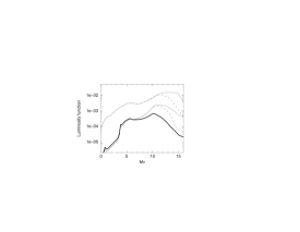
Figure 6: Upper curves: luminosity function in stars pc^-3 mag^-1 of the thin disc with an IMF slope $\alpha$ = 1.6. Solid line: single star luminosity function. Dashed line: system luminosity function. Lower curves: luminosity function of the thick disc. Solid thin line: single star luminosity function with $\alpha$ = 2. Dashed line: system luminosity function with $\alpha$ = 2. Thick line: single star luminosity function with $\alpha$ = 0.5.

The thin disc luminosity function that we used is a nearby luminosity function that does not take into account the fact that we may observe systems instead of single stars. Kroupa (2000b) showed that the difference between the nearby luminosity function and the system one comes from the binary fraction, nearby systems being computed as true single stars, while systems are not resolved in remote star counts. Hence, a correction is to be applied to the nearby luminosity function to take into account this effect in the counts. Following Kroupa, we applied a correction to the luminosity function used by the model in order to match the system luminosity function, as shown in figure 6 (upper curves). Only the deepest fields could be sensitive to this effect. When we apply this correction, the best fit thick disc parameters remain unchanged.

For the thick disc, the luminosity function considered in the model is the luminosity function of single stars. Knowing little about the binarity in the thick disc, we temporarily applied the same correction as for the thin disc on the luminosity function (see figure 6, lower curves). The best fit is obtained for the same density parameters h and df, but it slightly displaces the best IMF slope to $\alpha$ = 0.75. The likelihood values are slightly higher than those obtained with a single luminosity function (table 2).

6 Discussions and conclusions

We have estimated the thick disc density law parameters and mass function by using a wide set of data at high and intermediate galactic latitudes, in the visible and the near infrared. The best fit model has a scale height of 800 pc, a scale length of 2500 pc and a density of 10^-3 stars pc^-3 or 7.1 10^-4 M_⊙pc^-3 for Mv $\leq$ 8, that is 6.2% of the thin disc density. This result confirms the values obtained in 1996 from a smaller number of fields and mass ranges (Robin et al., 1996).

For the first time, we determined the thick disc mass function over a large mass range by the study of shallow star counts dominated by stars at the turnoff combined with deep star counts. The IMF of the thick disc seems to follow a power law dn/dm $\propto$ m^-0.5 in the mass range 0.2-0.8M_⊙. We found no evidence of a change of slope at lower masses, but we only have one field deep enough to constrain the IMF at low masses.

The only point of comparison for the thick disc mass function is the globular clusters of similar metallicities, where the conditions of star formation could be comparable. However, clusters are subject to bias with regard to the field because of possible mass segregation effects. From seven clusters, Piotto & Zoccali (1999) found a mean $\alpha$ of 0.89 at masses below 0.6M_⊙but the range covers 1.22 to 0.53, which is compatible with our measurements in the field.

Paresce & De Marchi (2000) found for similar clusters an indication of a lognormal IMF rather than a power law. If fitted by a power law in the mass range 0.3-0.8M_⊙, their IMF should be approximated by $\alpha$=1.6, but going down to $\alpha$=0.2 at m$<$0.3 M_⊙. The result clearly depends on the way an IMF, which globally is not a power law, is fitted in different mass intervals by portions of power laws. While our result seems not to favor a lognormal IMF compared to a power law slope in the mass range 0.2-0.8M_⊙, more data at lower masses may change our conclusion in the future.

Values of the spheroid IMF slope in the field range between 1.7$\pm$0.3 from a small local sample (Chabrier & Mera, 1997), 0.75 from HST star counts (Gould et al., 1998), and the higher value $\alpha$=1.9 determined from wide field star counts (Robin et al., 2000). However, the latter is valid at masses m$>$0.3M_⊙while the former go deeper to masses of about 0.1M_⊙and are less sensitive to higher masses because of the small size of the samples. A change of slope between intermediate masses and low masses, as found in the disc, may explain the apparent discrepancy, which is also partly due to the Poisson noise in these relatively small samples.

Scalo (1998) suggests it is not valid to rely upon a mean IMF, since variations are too high from one measurement to the other at the present time, but he identifies no tendency correlated with any physical parameter. On the other hand, Kroupa (2000a) finds that young clusters seem to have a steeper slope for m$<1$M_⊙and ancient globular clusters have $\alpha>0$ but closer to 0 than the field. He concludes that star formation produces relatively more low mass stars at later galactic epochs. His galactic field IMF for the disc has a slope of 1.3$\pm$0.5 at 0.1M_⊙$<$m$<$0.5M_⊙and 2.3$\pm$0.3 at 0.5M_⊙$<$m$<$1M_⊙.

If we consider the alpha-plot (figure 14 of Kroupa (2000a)), our measurement of a thick disc mass function similar to globular clusters seems to corroborate Kroupa’s conclusion. The thick disc mass function at low masses seems to be flatter than the thin disc and comparable with the spheroid. Figure 7 shows the alpha-plot versus metallicity for low-mass stars (m$<$3M_⊙), for which the effect is clearer. However, when taking into account other halo IMFs measured in the field, like Chabrier & Mera (1997), the correlation is less clear because of larger error bars due to the small size of the sample, as seen in the alpha-plot versus mass (figure 7). Clearly, the answer depends on a better determination of the IMF in the field, which can be done by exploring a larger mass range (going deeper) and having larger samples. This is promising in that several large scale surveys are on the way or planned for the near future.

Table 1: Characteristics of the selected fields.

Reference	Field	Area	Bands	Magnitude
	coordinates	(deg2)		range
Ojha et al. (1994a,b, 1996)	l=4∘, b=+47∘	15.5	B,V	V=15-17
	l=278∘, b=+47∘	20.8	B,V	V=16-18.5
	l=168∘, b=+48∘	7.13	B,V	V=15-18
Chiu (1980)	l=189∘, b=+21∘	0.10	B,V	V=18-20
Yee et al. (2000)	l=166∘, b=-55∘	0.39	V,I	V=17-20
Borra & Lepage (1986)	l=197∘, b=+38∘	0.25	B,V	V=20-22
Reid & Majewski (1993)	North Galactic Pole	0.30	B,V	V=19-22
DMS	l=129∘, b=-63∘	0.14	V,I	V=18-22
	l=248∘, b=+47∘	0.08	V,I	V=18-22
	l=337∘, b=+57∘	0.16	V,I	V=18-22
	l=77∘, b=+35∘	0.15	V,I	V=18-22
	l=52∘, b=-39∘	0.15	V,I	V=18-22
	l=68∘, b=-51∘	0.15	V,I	V=18-22
Bouvier et al. (1998)	l=117∘, b=-23∘	1.48	I,R	R=17-22.4
	l=206∘, b=+32∘	0.55	I,R	R=17-22
Sa57	l=69∘, b=+85∘	0.16	V,I	V=20-24

Table 2: Likelihood values obtained for the best fit parameters h and df when considering different thick disc IMF. The best fit parameters h and df are shown in figure 2 for the DENIS, deep and Sa57 fields in the case of an IMF following a single power law.

dn/dm	DENIS fields	deep field	SA57	all fields
m-0.5	-1830$\pm$200	-2500$\pm$150	-92$\pm$10	-5300$\pm$400
m-0.75	-1790	-2420	-88	-5250
m-1	-1760	-2370	-85	-5370
m-1.5	-1730	-2370	-79	-6260
m-2	-1730	-2480	-77	-8130
m-2 (m$>$0.6M⊙), m-1 (m$<$0.6M⊙)	-1730	-2570	-85	-7230
$\frac{1}{\mbox{m}}$exp-$\frac{[\mbox{log(m}/0.34)]^{2}}{2(0.4)^{2}}$ (lognormal)	-1710	-2510	-89	-6310
m-0.75 + binary correction	-1820	-2340	-87	-5100

Figure 2: Iso-contour likelihoods at 1 $\sigma$ as a function of scale height h and density df for different IMF slopes $\alpha$. Plus and dashed line: DENIS fields. Diamond and solid line: deep fields (V $\geq$ 20). Cross and dotted line: SA57.

Figure 3: Colour distributions of a DMS field in the magnitude bin I=20-22 and a DENIS field in the magnitude bin I=14-16. The dots show the observations. Thick lines are predicted number of stars by the model assuming $\alpha$ = 0.5, h = 800 pc and df = 1. Thin lines: $\alpha$ = 2, h = 800 pc, df = 1. Dotted lines: $\alpha$ = 1.7, h = 1100 pc, df = 0.7.

Figure 4: Iso-contour likelihoods at 1, 2, and 3 $\sigma$ as a function of scale height h and density df for all the fields together, considering an IMF slope $\alpha$ = 0.5.

Figure 5: Iso-contour likelihoods at 1 $\sigma$ as a function of scale height h and density df for different scale lengths l. Plus and solid line: fields towards the galactic centre. Diamond and dashed line: fields in the anticentre direction.

Figure 7: IMF slope $\alpha$ versus mass in M_⊙and metallicity. $\gamma$, $\Gamma$ and x are also power-law indices that may be used by other authors. Thin lines and filled symbols: globular clusters (triangles down: Paresce & De Marchi (2000), triangles up: Piotto & Zoccali (1999)). Thick lines and filled symbols: spheroid field stars (circles: Robin et al. (2000), diamonds: Chabrier & Mera (1997), squares: Gould et al. (1998)). plus: thick disc stars. Open circles: disc stars (Kroupa, 2001).