We examine the globular cluster systems (GCS) of a sample of 34 S0 galaxies from a WFPC2 snapshot survey in the V and I-bands. Of these 34 galaxies, 29 have measurable globular cluster systems. The mean color of the GCSs of individual galaxies vary from V-I=0.85 mag to V-I=1.17 mag. The average color of GCSs in all 29 S0 galaxies, V-I=1.00$\pm$0.07 mag, is similar to the value of V-I=1.04$\pm$0.04 derived for ellipticals in a companion paper. The mean metallicity of a cluster system is correlated to the luminosity (or mass) of the host galaxy, but is not dependent on the Hubble type. Our measurements of the local specific frequency, on the other hand, confirm that the cluster formation efficiency is a function of Hubble type. The mean local specific frequency of our sample within the WFPC2 field-of-view is 1.0$\pm$0.6, lower than S_N(Local)=2.4$\pm$1.8 derived for ellipticals in a similar analysis. Although we are able to confirm a bimodal color distribution in only one galaxy from the shallow ’snapshot’ images analyzed in this paper statistical tests suggest that 10-20$\%$ of S0s are bimodal at the present level of photometric accuracy. There are no significant trends in GCS properties with membership or location of the S0 host in a galaxy cluster. We have measured the turnover luminosity of the globular cluster luminosity function (GCLF) for the richest few GCSs and find the GCLF distances to be in agreement with other estimates. The globular clusters in S0 galaxies have average half-light radii of $\approx$2.6 pc which is similar to that of other galaxies, including our own.

1 Introduction

Globular clusters (GC) are among the most pristine objects in galaxies and hence provide invaluable insights into the chemical and kinematic conditions prevalent during the early epochs of galaxy formation. Just how early is presently a matter of some debate. Initial studies of the globular cluster systems of the Milky Way and other nearby galaxies led to the conclusion that all globular clusters are old, metal poor systems that were formed during the initial collapse phase of a protogalactic gas cloud. The subsequent discovery of metal rich GCSs and bimodal color (metallicity) distributions in some galaxies has led to much discussion about alternate mechanisms of globular cluster formation. Schweizer (1987) and Ashman $\&$ Zepf (1992) proposed that some GCs may be formed during the interaction or merger of galaxies. While Zepf $\&$ Ashman (1993) suggest that the bimodality in the color distribution is a natural consequence of the merger scenario, Forbes, Brodie & Grillmair (1997) favor multiple phases of cluster formation during the collapse of a gas cloud into a galaxy.

Only recently has it become possible to test these and other theories of globular cluster formation and evolution, due to the explosion in the number of observations of GCSs of external galaxies. However, much of the attention has been focused on cluster-rich ellipticals, with S0s being highly underrepresented in the sample of globular cluster systems studied to date. This is rather unfortunate since S0s may provide some essential clues to explain the small systematic differences between the GCSs of ellipticals and spirals, and may hold some of the keys to understanding the galaxy formation process. In this paper we attempt to rectify this imbalance by analyzing the cluster systems of 34 S0 galaxies from archival Hubble Space Telescope (HST) images. In a companion paper, Kundu & Whitmore (2001) (hereafter referred to as Paper I), we present a similar study of elliptical systems.

2 Observations and Data Reduction

This study is based on archival HST Wide Field and Planetary Camera 2 (WFPC2; hereafter WF=Wide Field Camera and PC=Planetary Camera) short exposure, ’snapshot’ images of nearby S0 galaxies. The list of program galaxies along with some salient information is presented in Table 1 (Note: Throughout this paper tables and figures are sorted by absolute magnitude of the host galaxy from Table 1, except in cases where distance-dependent effects are important, where they are sorted by distance). The galaxies were imaged with the F555W (1 image$\times$160s each) and F814W (2 images $\times$ 160s each) filters between Sep 6 1995 and May 3 1996.

We used the STSDAS utility GCOMBINE and the IRAF task COSMICRAYS to remove cosmic rays and hot pixels respectively from the F814W images, while we used only COSMICRAYS to reject cosmic ray events from the single F555W snapshots. We then identified cluster candidates using the technique described in detail in Kundu & Whitmore (1998). Briefly, DAOPHOT is used to identify sources using a low cutoff (1.5$\sigma$, where $\sigma$ is the standard deviation in the smoothest and faintest region of the image), then photometry is performed on each of the candidates, typically thousands per chip. The signal to noise for each detection is estimated by taking the ratio of the counts within a 0.5 pixel aperture to the rms noise in the sky background in the vicinity of the candidate. For this set of images we used a S/N cutoff of 3 to detect candidate clusters. We also used the ratio of the flux within an aperture of 0.5 and 3 pixels to weed out chip defects and compact background galaxies. Using a concentration criteria 2 $<$ $\frac{Counts_{3pix}}{Counts_{0.5pix}}$ $<$ 13 for the PC and 2 $<$ $\frac{Counts_{3pix}}{Counts_{0.5pix}}$ $<$ 10 for the WF, we identified cluster candidates that satisfied the selection criteria in both the F555W and the F814W image. Some of the S0 galaxies of later type have ongoing star formation in the disk and our detection algorithm identified many spurious objects in or near the disks of these galaxies. As most of the candidates in this region appear to be star forming regions, we masked out the point-like sources in the disks of NGC 1581, ESO 118-G034, NGC 2328 and NGC 3870. After correcting for the geometrical distortion (Holtzman et al. 1995a), we performed aperture photometry using a 3 pixel radius aperture for the PC and a 2 pixel radius aperture for the WF, using the median pixel value between 5 and 8 pixel radius as the sky background. Since the profiles of the cluster candidates are slightly broader than a stellar PSF, we used the distance-dependent aperture corrections computed in Paper I. To maintain consistency with Paper I we adopted photometric zeropoints of 22.573 mag and 21.709 for the PC and applied small color correction terms from Holtzman et al. (1995b) to convert the F555W and F814W magnitudes to Johnson V and Cousins I respectively. Since the zeropoints for each of the WF chips are offset slightly from the PC values we added the small differences quoted in the HST data handbook (1997) to the above values before applying the color correction terms to the candidate objects in the WF (see Paper I for details). We corrected for the foreground Galactic extinction in the direction of each of the observed galaxies using the A_B (Burstein & Heiles 1982) values quoted in the NED extragalactic database and the reddening curve from Mathis (1990). The V-band extinctions are listed in Table 1. A careful observation of the V, I and V-I images revealed that internal reddening is not an issue in most of the galaxies in our sample. Significant dust lanes are only seen in the disks of the very late type S0s, but as indicated above we already exclude these regions because of confusion due to star forming regions. A few of the earlier type galaxies have weak dust lanes in a very small region around the nucleus - of the order of a few arcsecs - which does not affect the global properties of the observed cluster systems. We did not correct for the Charge Transfer Efficiency (CTE) gradient across the chips as the CTE problem is expected to be minimal in the presence of the strong galaxy background in most of our sample objects. (Holtzman et al. 1995b; Whitmore & Heyer 1997). Even in regions of low background the CTE corrections are expected to be small ($\sim$0.02 mag) at the epoch of these observations (Whitmore et al. 1999).

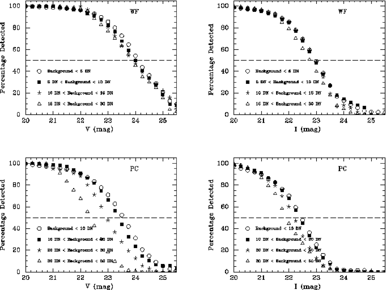
Figure 1: Completeness curves for globular clusters in the V (F555W) and I (F814W) images for objects with a V-I color of $\sim$1.0 mag as a function of background counts (see text for details). Even though the V-band images are only 160s snapshots, the 50% completeness limit is at about V=24 mag, comparable to deep ground-based images.

For statistical studies of globular cluster systems it is necessary to quantify the photometric incompleteness of our detections i.e. the ability to detect candidates as a function of magnitude. Since the exposure time for all of our images is identical, the completeness curve for each galaxy is expected to be only a function of the galaxy background. This makes our task a little simpler in that we only need to measure the detection threshold for a representative sample of galaxies. We selected a random set of galaxies that spanned a large range of background counts and added simulated clusters, which we then attempted to detect with the routine used to identify the cluster candidates. We only added 100 objects at random positions in each chip during each simulation - in both the F555W and F814W images - to ensure that there was negligible overlap of objects. Moreover, since a preliminary examination of our data showed that the colors of most of the candidate globular clusters are in a narrow range of values around V-I$\approx$1.0 as expected for old globular clusters, we allowed our simulated objects to have random colors between 0.8$<$V-I$<$1.3. In all, we added approximately 35000 objects using the IRAF task ADDSTAR. The completeness curves derived from these tests are presented in Fig 1. The typical 50% detection threshold is V$\approx$23.4 mag in the PC, and V$\approx$24 mag in the WF. The I-band detection limits are $\approx$1 mag brighter than those in the V-band. These values are comparable to the deepest ground-based observations, even though this analysis is based on ^′snapshot^′ 160s exposures in the V-band and 320s in the I-band.

Globular cluster systems of galaxies outside the local group can be measured statistically as an overdensity of point-like objects as compared to a blank field a small distance from the galaxy. We do not have off-galaxy images for this set of observations, but the superior angular resolution of the HST makes this almost redundant since globular clusters can generally be distinguished both from unresolved foreground stars and background galaxies. A judicious color cutoff is used to further eliminate most of the contaminants. At low galactic latitudes, however, there may be large number of foreground stars in the field of view. Also, cluster systems with less than $\sim$50 clusters are likely to have significant contamination. We have noted the potential contamination problem in specific galaxies in the next section.

3 Results and Discussion

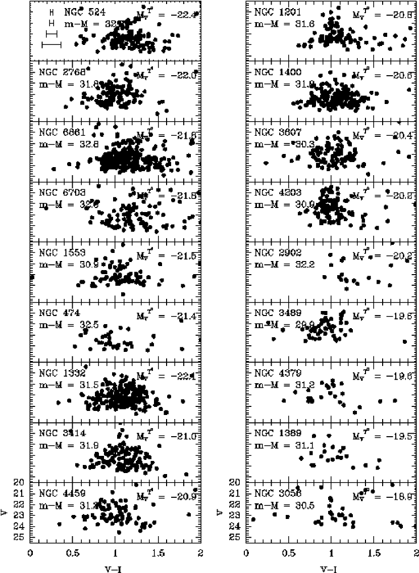
Figure 2: Color-magnitude diagrams for the globular cluster candidates in the program galaxies. Most of the candidates lie in a narrow range of color between 0.5$<$V-I$<$1.5. The distances (from velocities) and magnitudes are from Table 1. The galaxies are sorted by the absolute magnitude of the host.

The color-magnitude diagrams of the point-like objects in the program galaxies are shown in Fig 2. A majority of the cluster candidates lie in a narrow range of color between 0.5$<$V-I$<$1.5 with a mean color near V-I $\approx$ 1.0 mag, which is typical for old GCSs.

In the galaxies which have significant cluster populations one can discern that the mean of the color distribution is roughly constant with magnitude. The dispersion of the colors does seem to increase for the fainter objects, but this is most likely a reflection of the larger photometric uncertainties at these magnitudes. Galaxies at low galactic latitudes (NGC 404, NGC 1201, NGC 2328, NGC 2902, NGC 3056 & NGC 6703) appear to have a larger fraction of objects redder than V-I = 1.5 mag, which can be attributed to contamination by foreground stars. In order to help filter out the few remaining contaminants, largely foreground stars and background galaxies, we shall consider only objects within the color range 0.5$<$V-I$<$1.5 to be bona fide cluster candidates and all objects outside this range to be ^′background^′ objects (meaning both foreground and background interlopers).

We inspected the spatial distribution of the cluster candidates in each of the 34 galaxies and found that the density distribution of the cluster candidates in most of the galaxies was roughly centered on the nucleus of the galaxy, further suggesting that the candidates are bona fide clusters associated with the galaxy in question. The cluster candidates of four galaxies (ESO 118-G034, NGC 2328, VCC 165 and IC 3131) did not appear to be spatially correlated to the underlying galaxy, which leads us to believe that either these galaxies do not have significant cluster systems within our field of view or they are heavily contaminated by ^′background^′ objects. We shall not discuss the globular cluster systems of these galaxies in this paper except in $\S$3.3 where we place limits on the specific frequency. NGC 404 presents a unique problem since the luminosity and color distribution look very different from those of the other S0s, with a sudden increase in both the number of objects and the color spread of the candidates near V$\approx$24 mag (or I$\approx$23.5). We suspect that we are actually observing the tip of the red giant branch in this nearby galaxy. If we adopt the Lee, Freedman & Madore (1993) value of M_I $\approx$ -4.0 mag for the absolute magnitude of the tip of the red giant branch the distance modulus to the galaxy is m-M $\approx$ 27.5 mag. Thus we suspect that NGC 404 is probably at a distance of $\approx$ 3 Mpc, and not 10 Mpc as suggested by Wiklind & Henkel (1990) from their arguments based on the morphological characteristics and molecular gas content of the galaxy.

Twelve of the 29 galaxies have more than 50 candidate clusters in the field of view of our images. The other 17 may be severely affected by small number statistics and/or contamination. In subsequent sections we have analyzed the cluster properties of all 29 galaxies with appropriate error estimates, allowing the reader to make the subjective decision of which galaxies have ’believable’ cluster systems. We note that we have included some of the numbers derived for the NGC 4550 globular cluster system in Paper I in relevant sections of this analysis of S0 galaxies. Although NGC 4550 is a SB0⁰, it was not observed as part of the snapshot survey. Unlike the snapshot data set studied in this paper, the reduction and analysis techniques employed for the deeper NGC 4550 images were identical to the elliptical galaxies in Paper I. Hence we decided that it would be more appropriate to include it in Paper I. When we weigh the properties of S0s vis-a-vis ellipticals we take care to include NGC 4550 in the S0 sample.

3.1 The Color and Metallicity Distributions

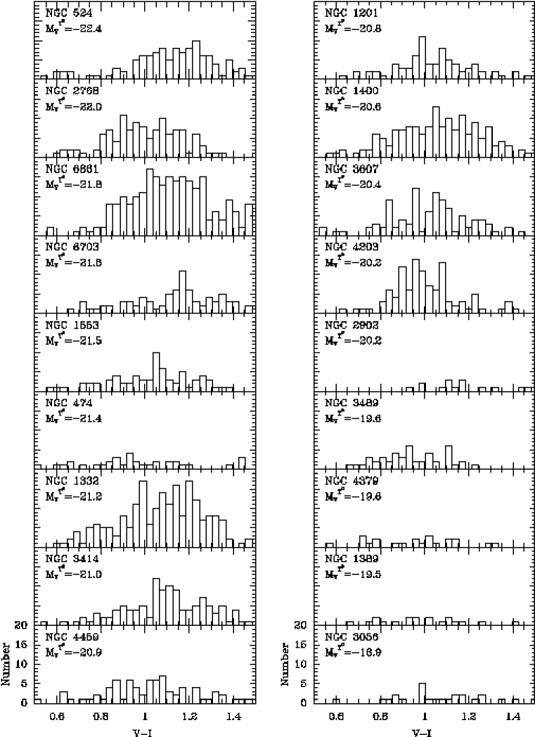
Figure 3: Color distributions of the globular cluster candidates in the 29 galaxies with measurable cluster systems. Statistical tests indicate that NGC 2768 is the only galaxy in our sample with a confirmed bimodal color distribution. The small number of cluster candidates and the uncertainties in the photometry arising from the short exposure times make it impossible to statistically confirm, or rule out, bimodality in most cases.

The V-I color distributions of the cluster candidates in the range 0.5$<$V-I$<$1.5 are shown in Fig 3. The spread in GC colors in each galaxy is V-I$\sim$0.5 mag. This dispersion in color cannot be attributed to the photometric errors alone (typically $\approx$0.15 mag), hence it represents an actual variation in broad-band color from cluster to cluster.

The mean colors of the globular cluster candidates in the color range 0.5$<$V-I$<$1.5 are listed in Table 2. The error estimates quoted are the formal uncertainties in the means (Note - Throughout this paper we have used the following convention in quoting uncertainties: The number following the $\pm$ sign is the standard deviation, while a number in parentheses refers to the uncertainty in the mean). Stellar population modeling shows that the color difference between globular clusters is dominated by age effects for clusters younger than $\sim$1 Gyr old, and by metallicity effects otherwise (Worthey 1994; Bruzual & Charlot 1993 etc). Since the GC color and luminosity (§3.2) distributions of our sample are fairly typical of old ($>$$\sim$8 Gyr) cluster systems, we can safely attribute the color spread predominantly to metallicity variations. The mean metallicities of the GCSs, adopting the transformation equation based on Galactic clusters from Kundu & Whitmore (1998), are also listed in Table 2. However, we note that the faintest clusters (in the V-band) in some of the galaxies in Fig 2 are selectively redder. A corresponding color-magnitude diagram plot in the V-I, I plane would show that the faintest clusters in the I-band are selectively bluer. This is an artifact of the cluster identification method which required that the cluster candidate be present in both the 160s V image and the deeper 320s I image. Since this bias only occurs at the faint end of the luminosity function where the completeness is low, the overall effect on the mean color is expected to be quite small. In order to quantify this uncertainty we calculated the mean colors for various cutoff magnitudes in V and I. The average offset in the mean color of the raw data and the magnitude limited samples is only $\sim$0.02 mag. Therefore we are confident that the mean colors are largely unaffected by selection biases.

In Table 2 we also indicate the number of cluster candidates within the color range of typical clusters, N_cand, and the number of sources with colors between 0.0$<$V-I$<$0.5 or 1.5$<$V-I$<$2.0, N_bg. The point-like objects in the latter subset are likely to be largely contaminants. One might reasonably infer that galaxies with large values of N_bg also have significant number of contaminants in the color range of clusters. Therefore, in calculating the mean color of GCs in S0s we only consider systems with N_bg/N_cand$<$0.25. The average color of our S0 sample is V-I=1.00$\pm$0.07 (0.01) mag which corresponds to a mean metallicity of [Fe/H]=-1.1$\pm$0.3 (0.07) dex. This is very similar to the value of V-I=1.03$\pm$0.04 (0.1) derived for ellipticals in Paper I.

Up to this point we have been discussing only the average metallicities of the cluster systems; the shapes of the color histograms may also hold vital clues about the formation history of S0 galaxies. One of the most significant discoveries in globular cluster research in recent times is that the broad-band color distribution of 25-50$\%$ of the early type galaxies studied are bimodal (e.g. we showed in Paper I that at least 50% of ellipticals have bimodal GCS color distributions). This effect, which is usually interpreted as a bimodality in the metal abundance of the cluster systems, suggests that globular clusters have formed during two distinct epochs in the metal enrichment histories of these galaxies. However there is much disagreement about the physical mechanism that triggers the second burst of cluster formation. Schweizer (1987) and Ashman $\&$ Zepf (1992) proposed that GCs may be formed during the interaction or merger of galaxies. While Zepf $\&$ Ashman (1993) suggest that the bimodality in the color distribution is a natural consequence of the merger scenario, Forbes, Brodie & Grillmair (1997) favor multiple phases of cluster formation during the collapse of a gas cloud into a galaxy.

The search for bimodality in the color distribution of globular cluster systems has largely been limited to elliptical galaxies; little is known about the distributions in S0 galaxies and the implications on formation models. To date, NGC 1380 & NGC 3115 are the only S0 galaxies confirmed to have a bimodal color distribution (Kissler-Patig et al. 1997; Kundu & Whitmore 1998). Since these are also the only S0 galaxies in which a deep study of the color distribution of the GCS has been made it is unclear what percentage of S0 galaxies are bimodal.

An inspection of the histograms of the color distributions in Fig 3 reveals no candidates with strikingly obvious bimodality. In order to objectively test whether the unbinned distributions have multiple modes we applied the KMM mixture modeling algorithm of Ashman, Bird & Zepf (1994), which tests the suitability of modelling a distribution with multiple Gaussian sub-populations. Since the KMM algorithm is very sensitive to outliers we did not attempt to use it on systems with fewer than 50 globular cluster candidates, where small number statistics and contamination by background and foreground objects may lead to false confirmations of multiple peaks. KMM tests on the more cluster-rich systems revealed that only NGC 2768 has a statistically significant probability of having a bimodal color distribution, with peaks at V-I=0.92 mag and V-I=1.12 mag. On the face of it, it would appear that the fraction of S0 galaxies with multimodal color distributions is much smaller than that of elliptical galaxies, but we hasten to add that we are limited by the small number statistics and the photometric uncertainties arising from the short exposure times of this snapshot survey. Ashman et al. (1994) show that for sample sizes of 100-200 objects the photometric uncertainties should be a factor of $\sim$2.5-3.0 less than the expected separation between the peaks for the KMM algorithm to reliably detect or reject bimodality. Given that in most galaxies with bimodal color distributions studied to date the difference in the peaks is of the order of V-I$\approx$0.2 mag and that the typical mean uncertainty in color in our data sets is V-I$\approx$0.15 mag we do not expect to detect bimodality in many individual systems.

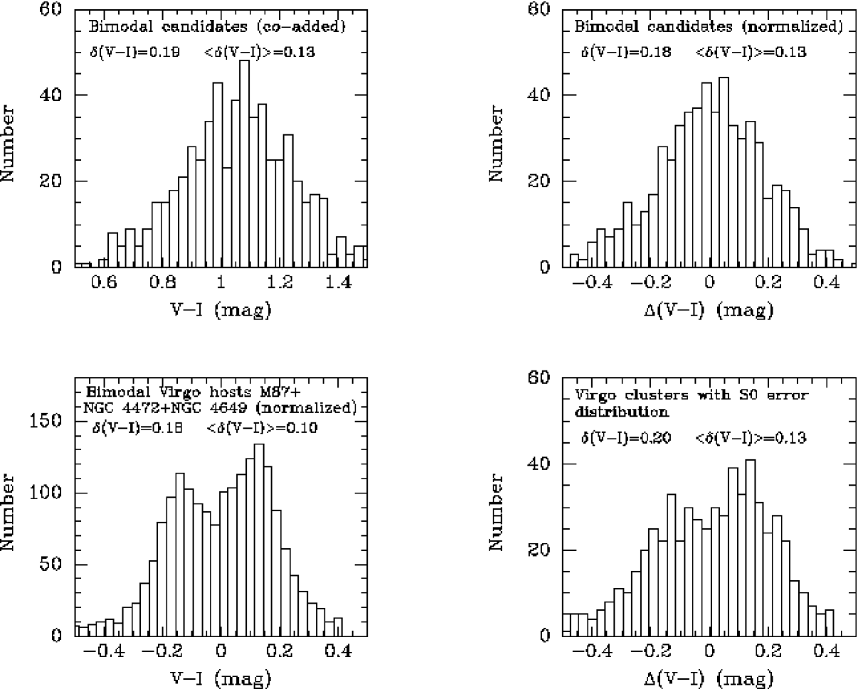
Figure 4: Top left: The co-added color distribution of the 5 galaxies with probable bimodal color distributions; Top right: The co-added color distribution of the 5 galaxies with probable bimodal color distributions normalized to a common mean color of V-I=0; Bottom left: The normalized color distribution of M87, NGC 4472 & NGC 4649 from the analysis of Kundu et al. (1999) and Paper I show obvious bimodality; Bottom right: The subset of the normalized color distribution of the Virgo galaxies with the exact same uncertainty distribution as the bimodal S0 candidates in the upper panel.

Based on a visual inspection of the color-magnitude diagrams of the clusters and the KMM test results the following galaxies appear to be promising candidates for bimodality : NGC 1201, NGC 1332, NGC 3489, NGC 4459, and possibly NGC 6861. Although KMM tests suggest that two Gaussians fit the color distributions of these galaxies better than a single Gaussian at a 95% level of confidence in these systems the homoscedastic (populations forced to have equal variances) and heteroscedastic partitions (populations allowed different variances) yielded red and blue population with significantly different partitions and mean colors (different by $\sim$0.05 mag). Given the low number statistics and the photometric uncertainties we do not consider these partitions to be very reliable. In order to improve the number statistics and search for stronger evidence of bimodality we co-added the likely bimodal systems. In the top left panel of Fig 4 we plot the co-added color distributions of NGC 1201, NGC 1332, NGC 3489, NGC 4459 and NGC 2768. Though we see no obvious sign of bimodality in this plot, it does not necessarily mean that the individual systems are unimodal. It is possible that the bimodal peaks are at different locations in each galaxy. In order to somewhat alleviate this problem we shifted the color distribution of each of the individual GCSs to a common mean of V-I=0 and then co-added them. The V-I histogram (Top right of Fig 4) still shows no convincing evidence of bimodality. A KMM test on the co-added, normalized distribution suggests that two Gaussians with (normalized) peaks at V-I = -0.08 and 0.09, with roughly equal number of candidates in each Gaussian, fits the data better than a single Gaussian at better than a 95% confidence level. However, a careful visual inspection of the distribution reveals no obvious peaks at these locations. Thus one may only conservatively conclude from the KMM tests that the color distribution is broader i.e. more flat-topped than a Gaussian. The fact that the standard deviation in the mean (normalized) color, $\delta$$<$V-I$>$ = 0.18 is larger than the mean of the photometric uncertainty of individual clusters, $<$$\delta$(V-I)$>$ further supports this conclusion. In order to further test the significance of the color spread in S0s we compare them with confirmed bimodal elliptical GCSs. In the lower left panel of Fig 4 we plot the co-added, normalized color distribution of 3 Virgo galaxies, M87 (Kundu et al. 1999), NGC 4472 and NGC 4649 (Paper I). KMM tests indicate that the distribution is well described by Gaussians with peaks at V-I = -0.12 and 0.10 at a confidence level of 95%. Next we selected the subset of the Virgo clusters with the exact same photometric uncertainty distribution as the co-added S0s by matching each S0 cluster with a Virgo GC with the same - or as close as possible - computed photometric uncertainty (taking care that each Virgo globular cluster is selected only once). The mean difference in color uncertainties between individual S0 clusters and Virgo clusters is -4.1$\times$10^-5 $\pm$ 0.001, confirming that the uncertainty distributions are indeed almost identical. The color distribution of this Virgo subset is shown in the bottom right panel of Fig 4. Clearly the raw histogram does not show very strong evidence for bimodality. However, KMM tests confirm that the Virgo clusters with S0 error distribution are inconsistent with a unimodal distribution, and can be better fit by Gaussians with peaks at -0.11 and 0.11. This gives us more confidence in the KMM tests for the normalized S0 candidates and suggests that these S0s may indeed have non-unimodal color distributions. However, we do note that although by definition the Virgo subset has the same $<$$\delta$(V-I)$>$ (0.13) as the S0 distribution, the standard deviation in the mean color of the Virgo globular clusters is slightly larger (0.20 as opposed to 0.18). We conjecture that this indicates that even though the S0 systems may be bimodal the ratio of red to blue clusters is significantly different from the 1:1 mix typical of giant ellipticals.

Thus, considering the galaxies in our sample plus NGC 3115, NGC 1380, and NGC 4550 the only other S0 galaxies which good data on the color distribution exists, we conclude that at least 10$\%$ of S0 galaxies have confirmed bimodal color distributions, at the present lavel of photometric accuracy. In light of the discussion in the previous paragraph we are unable to definitively rule out bimodality in most of the other cases due to small number statistics and relatively large photometric errors. We suggest that at least another 10$\%$ of S0s may be bimodal.

3.2 The Globular Cluster Luminosity Function

The shape and turnover magnitude of the globular cluster luminosity function has been found to be nearly constant over a wide range of galaxies and environments (Harris 1991). While the theoretical basis for this phenomenon remains unclear, this is a remarkable result which implies that for any reasonable range of M/L ratio the underlying mass distribution of globular clusters is similar in most galaxies. This can be exploited to determine distances to galaxies (e.g. Jacoby et al. 1992; Whitmore 1996). In Paper I we improved upon previous estimates of the GCLF parameters - M${}_{V}^{0}$ = -7.41 (0.03), M${}_{I}^{0}$ = -8.46 (0.03) and $\sigma$ $\approx$ 1.3 for a Gaussian fit - and showed that the GCLF is an excellent distance indicator for elliptical galaxies. There are lingering doubts that the turnover magnitude varies with Hubble type (e.g. Secker 1992), although Ashman, Conti & Zepf (1995) (hereafter ACZ) ascribe these differences to metallicity effects.

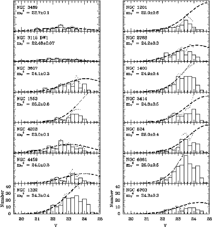
Figure 5: a: The V-band globular cluster luminosity function of the 14 richest cluster systems sorted by Table 1 distances. Only cluster candidates in the range 0.5$<$V-I$<$1.5 and V$>$(m-M)-11.0 have been selected in order to minimize contaminating sources. The dotted lines trace the completeness corrected distribution up to the 50$\%$ completeness limit. The dashed lines mark the best fit Gaussian curve. b: The corresponding GCLFs in the I-band. The GCLFs are typically $\sim$1 mag brighter in I.

Most of the galaxies in our sample do not have enough clusters for us to determine the peak of the GCLF accurately so we choose to study only the 14 richest cluster systems. The luminosity functions of these galaxies in the V and I-band, sorted by the distance modulus in Table 1, are plotted in Fig 5. In each case we have plotted the GCLF only for the candidates that are fainter than V=(m-M)-11.0 in order to limit the effect of outliers - most likely foreground stars - on the luminosity function.

It is apparent from Fig 1 the completeness curves are background dependent and also vary between the WF and PC chips. Following the prescription laid out in detail in Paper I we computed a background count and cluster density weighted completeness curve for each of the candidates. The 50% completeness limit in most galaxies is at V$\approx$24 and I$\approx$23. The completeness corrected GCLFs, up to the respective 50% completeness limit of each GCS, is shown by the dotted lines in Fig 5. As in Paper I we calculated the parameters of the best fit Gaussians to the GCLFs by using the IRAF task NGAUSSFIT and varying the width (0.18 to 0.25 mag) and positioning of the bins, the cutoff magnitude at the faint end (40$\%$ to 55$\%$ completeness), and $\sigma$ (1.1 to 1.5). For the adopted mean $\sigma$ of 1.3 we calculated the average turnover magnitude, the amplitude of the Gaussian and the associated standard deviation from 40 individual fits. The best fit Gaussian ($\sigma$=1.3) GCLF is plotted using dashed lines in Fig 5 and the turnover magnitude is listed in Table 3. The uncertainties in the turnover reported in Table 3 are the standard deviations from the mean of the 40 fits to the GCLF and are a good measure of both the systematic and formal uncertainties.

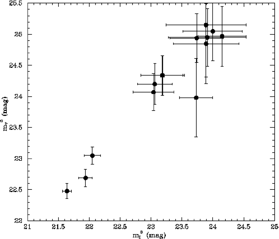
Figure 6: The turnover luminosity of the best fitting Gaussian to the GCLF in the V-band, m${}_{V}^{0}$ vs the turnover luminosity in the I-band, m${}_{I}^{0}$. The turnover luminosities in the two filters are well correlated.

By and large, the peak of the cluster distribution migrates to fainter magnitudes for more distant galaxies in Fig 5. We point out that the distances quoted are from Table 1, which have have been derived from the velocity and are not likely to be very accurate. In Fig 6 we plot the turnover luminosity in the I-band vs that in the V-band. It is apparent that m${}_{V}^{0}$ and m${}_{I}^{0}$ are tightly correlated, and within the uncertainties follow a linear relationship. The uncertainties are larger for the more distant, fainter systems as is only to be expected from the completeness limits.

In order to test the suitability of S0 GCLFs as distance indicators, we would ideally like to compare the turnover magnitude with distance moduli obtained by other methods and measure the constancy of the turnover. Unfortunately only a couple of galaxies in our sample have reliable independent measurements using other distance indicators (see below). Therefore, we opt instead, to adopt the absolute turnover magnitudes derived for ellipticals in Paper I and check for consistency between the derived S0 GCLF distance moduli and other distance estimates. The distance moduli to some of the galaxies reported in the literature are listed in column 5 of Table 3. Most of the reported distances are from Prugniel & Simien (1996). As in Table 1, these distances are based on recessional velocities but they incorporate Virgocentric infall and great attractor corrections using an independent model. For NGC 1400 we report the average fundamental plane distance modulus in the I (31.67$\pm$0.14) and K’(32.07$\pm$0.25) band from Jensen, Tonry & Luppino (1998). Columns 6, 7 and 8 of Table 3 show the computed GCLF distances in the V, I and mean distance respectively, for the adopted Paper I turnover magnitudes of M${}_{V}^{0}$=-7.41$\pm$0.03 and M${}_{I}^{0}$=-8.46$\pm$0.03. We do not compute distances for galaxies with mean GCLF uncertainties greater than 0.3 mag as these are likely to be very unreliable. The GCLF distances appear to be consistent with other distance estimates for our sample of S0s, and by extension there seems to be no obvious offset between the absolute turnover magnitudes of ellipticals and S0s. The mean difference between the GCLF distance moduli and those from the literature (column 5 of Table 3) is 0.01$\pm$0.4, quite similar to the difference between the distances from Table 1 and those reported in the literature, 0.07$\pm$0.5. More accurate independent distance estimates of S0 galaxies and deeper observations of GCLFs are needed to further establish the accuracy (or applicability) of the turnover magnitude as a distance indicator in S0s. However, we note that the turnover magnitude of NGC 3115, the S0 galaxy with the best determined GCLF to date, yields a distance measurement that is compatible with other estimates and falls within the range of values derived by the tip of the red giant branch, planetary nebula luminosity function and surface brightness fluctuation methods (Kundu & Whitmore 1998).

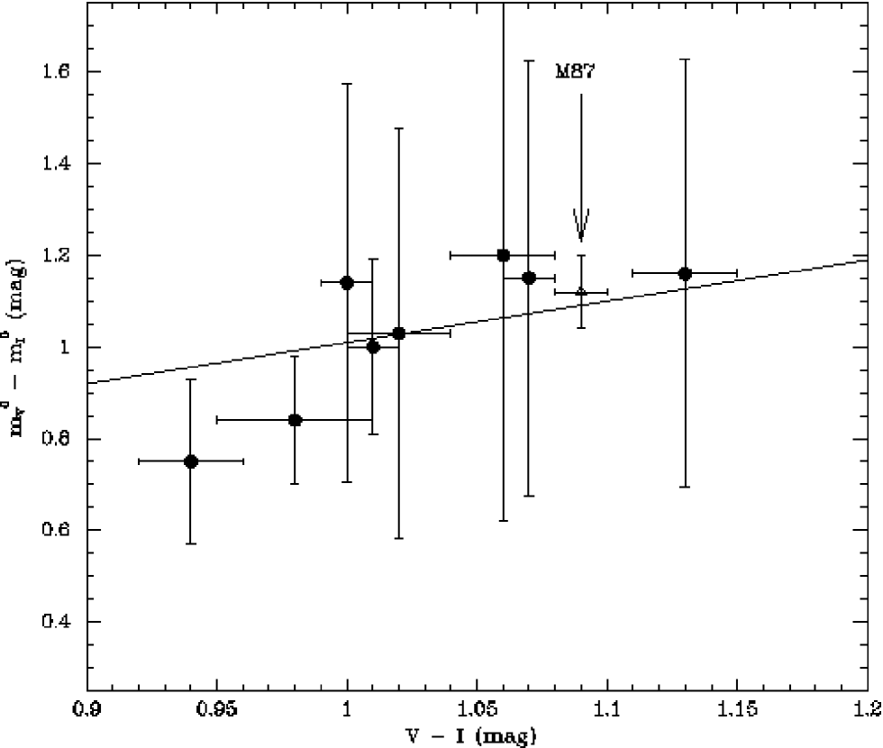
Figure 7: The difference between V and I-band turnovers as a function of cluster color (metallicity). m${}_{V}^{0}$-m${}_{I}^{0}$ increases with color, as predicted by the Ashman, Conti, & Zepf (1995). The dashed line tracing the best-fit straight line from a similar analysis of ellipticals in Paper I is in good agreement with the observed trend.

Ashman, Conti & Zepf (1995 hereafter ACZ) showed that for a universal globular cluster mass function the peak of the GCLF is slightly dependent on the metallicity. Both the V and I-band turnovers migrate to fainter magnitudes in more metal-rich systems, the effect being larger in V. In Paper I we showed that m${}_{V}^{0}$-m${}_{I}^{0}$ does increase with the color (metallicity) of the cluster system, consistent with the ACZ estimates. Fig 7 is a corresponding plot of m${}_{V}^{0}$-m${}_{I}^{0}$ as a function of mean cluster color for the S0 systems for which GCLF distances are reported in Table 3. For comparison we also plot a point for M87 and the best fit line from our elliptical sample, (m${}_{V}^{0}$ - m${}_{I}^{0}$) = 0.11 + 0.90$\times$(V-I). Rather surprisingly, despite the large uncertainties in the turnover magnitudes derived from the shallow images of S0s, within the uncertainties the S0 sample is consistent with the metallicity trend of the elliptical sample. This indicates that systematic errors dominate the GCLF determinations of the short exposure S0s, and that these errors are correlated in the V and I-band, i.e. Given that the ratio of exposure times in F555W & F814W is exactly the same for the entire S0 data set, the ratio of the fraction of the V-GCLF vs the I-GCLF used for our Gaussian fits is roughly the same for galaxies at all distances in our sample. We suggest that the color dependence of m${}_{V}^{0}$-m${}_{I}^{0}$ indicates that the shape of the bright end of the GCLF is similar in both the V and I-bands. Therefore even in the most distant candidates in which the 50% completeness limit falls far short of the turnover magnitude the difference in m${}_{V}^{0}$-m${}_{I}^{0}$ can be determined more accurately than the individual turnovers in either filter. This would also explain why m${}_{V}^{0}$ and m${}_{I}^{0}$ appear extremely well correlated, despite the large uncertainties, even for the faintest GCSs.

Based on the analysis of the globular cluster luminosity functions of our S0 sample we conclude that within the uncertainties, the turnover magnitude of S0s are consistent with other distance measurements, and that the bright end of the GCLF luminosity function has a similar shape in the V and I-band.

3.3 Specific Frequency

The specific frequency, S_N, is defined as the number of globular clusters per unit galaxy luminosity normalized to M_V=-15 (Harris & van den Bergh 1981):

S_N=N_t 10${}^{-0.4(M^{T}_{V}+15)}$

where N_t is the total number of clusters and M${}^{T}_{V}$ is the total magnitude of the underlying galaxy. Given the limited field-of-view of the WFPC2 our images only cover a portion of the sample galaxies. Therefore we cannot measure the global specific frequency of the galaxy directly. We can, however, derive the local value of S_N within the HST field-of-view using the total V-band magnitude of the galaxy in our image and the projected total number of clusters in the region. Our method of calculating these two quantities and the underlying assumptions are outlined below.

The total number of candidates with colors in the range 0.5$<$V-I$<$1.5 detected in each galaxy and the number of objects with colors in the range 0$<$V-I$<$0.5 or 1.5$<$V-I$<$2.0 are listed in Table 2 under the headings N_cand and N_bg respectively. We then calculated histograms of the candidate objects brighter than V=24 mag and corrected them by the completeness curves derived in the previous section to arrive at the projected total number of candidate objects with V$<$24 mag within our field-of-view, N_V<24. This number is roughly the same as N_cand since the number of objects fainter than V=24 mag is small and this is effectively offset by the completeness correction.

Next we must account for the contamination by background and foreground sources. Since we do not have off-galaxy images we attempt to correct the contamination in color space. For the 4 galaxies which appear to have no cluster candidates we found that N_V<24 is roughly equal to 1.5$\times$N_bg. Assuming that this is a typical background in all our galaxies we subtract 1.5$\times$N_bg from N_V<24 to arrive at the total number of contamination and completeness corrected objects brighter than V=24 mag in our field-of-view. As in the previous section, we adopt the parameters of a Gaussian GCLF describing elliptical galaxy GCSs, $\sigma$=1.3 and a turnover luminosity of M${}_{V}^{0}$=-7.41. Using the distance estimates from Table 1 to calculate the expected fraction of clusters brighter than M_V=24 mag and thence the projected total number of clusters within our field-of-view, N_Tot. We estimate that the uncertainty in the total number of clusters is the sum in quadrature of the uncertainty from Poisson statistics, $\sqrt{N_{cand}}$, and the uncertainty due to contamination, N_Tot $\times$ ($\frac{N_{bg}}{N_{cand}}$). As a check, we calculated the integrated area under the GCLF and the associated errors for the candidates with well defined luminosity functions in the previous section, in a manner similar to the Paper I analysis. While the total number of clusters returned by both methods was similar, the uncertainty in the total number of clusters was $\sim$2 times as large using the latter method. Thus the uncertainties in the total number of clusters, and hence the uncertainty in the local value of S_N is typically underestimated by a factor of 2 in this paper when compared to the analysis of the elliptical sample.

Determining the integrated magnitude of the galaxy is more problematic because nearly all of our galaxies are spatially larger than the WFPC2 field-of-view, making background subtraction impossible. Moreover, we have only one F555W (V-band) image for each galaxy which means that the cosmic ray rejection is far from ideal. While this does not affect aperture photometry of the point-like globular clusters - the likelihood of a cosmic ray event being superposed on a point source is very slim - surface photometry can be significantly degraded. Instead, we calculated the integrated light within the F814W image, subtracted ’the typical sky background’ in the I-band from the WFPC2 Handbook (0.0544 e^-s^-1pixel^-1 in the WF and 0.011 e^-s^-1pixel^-1 in the PC - WFPC2 Handbook) and adopted a value of V-I=1.2$\pm$0.1, which is fairly typical of S0 galaxies, to determine the integrated V magnitude of the program galaxies. We assumed that the uncertainty in the surface photometry is of the order of the subtracted ^′background^′, plus an additional 0.1 mag due to the transformation from I to V and propagated this in the calculation of the uncertainty in the specific frequency. In order to check the accuracy of the surface photometry we compared our derived V-band photometry in small apertures with published aperture photometry. For an aperture of 29.8^′′ in NGC 6861 we derived V = 11.84 mag, compared to the published value of 11.88$\pm$0.02 mag (Sandage & Visvanathan 1978). For apertures of 25.9^′′, 29.8^′′ and 35.6^′′ in NGC 1553 we calculated V = 11.16 mag, 11.04 mag and 10.91 mag, in good agreement with the published values of 11.19$\pm$0.02 mag, 10.94$\pm$0.02 mag and 10.84$\pm$0.03 mag respectively (Persson, Frogel & Aaronson 1979; Sandage & Visvanathan 1978; Sandage 1975). The published numbers of V = 11.53$\pm$0.02 mag and 11.46$\pm$0.02 mag (Persson et al 1979; Sandage & Visvanathan 1978) for 25.9^′′ and 29.8^′′ apertures are consistent with our values of 11.45 mag and 11.36 mag in NGC 1332. Thus the uncertainties in the integrated magnitude of the hosts adopted by us seems to be reasonable estimates.

The local specific frequency in the inner region of the galaxies is listed in Table 2 along with the global values for the candidates that have previously been observed in ground-based studies. The local specific frequency varies from 0 for galaxies with no measurable cluster systems to 6.8 for the cluster rich dwarf NGC 3115 DW1, with a mean value of 1.0$\pm$0.6 (0.1) for all S0s with uncertainty in individual local specific frequencies, $\delta$S_N(Local), less than 1.5. This is lower than the local specific frequency of 2.4$\pm$1.8 (0.4) derived for elliptical galaxies in Paper I and is consistent with previous observations that the specific frequency of S0s is lower than that of ellipticals (Harris 1991). The large spread in S_N from galaxy to galaxy is real, and any unified theory of globular cluster formation must be able to account for vastly different efficiencies of globular cluster formation in individual galaxies. In this connection NGC 3115 DW1 is an especially interesting case. As has previously been pointed out (Hanes & Harris 1986; Durrell et al. 1996; Puzia et al. 2000) this dwarf galaxy appears surprisingly cluster rich. This can also be clearly observed in the color-magnitude plots in Fig 2 which are sorted by the absolute magnitude of the galaxy. While the density of clusters roughly increases with the brightness of the host galaxy, NGC 3115 DW1 has an anomalously overdense system as compared to other galaxies of similar size.

The local specific frequencies derived in both Paper I and this analysis are of course measured within the WFPC2 field-of-view, hence a larger fraction of the cluster population and galaxy light is included for the more distant galaxies. While specific comparisons between individual galaxies in either sample may not yield very meaningful results, on average both the S0 and the elliptical hosts are distributed over a similar distance range [(m-M) = 31.4$\pm$0.7 for ellipticals and (m-M) = 31.2$\pm$1 for S0s], hence we can legitimately make comparisons between the average properties of both samples. Also, in consort with published values, it is possible to study the radial properties of the specific frequency of each galaxy. The local specific frequencies calculated here add to this reference list.

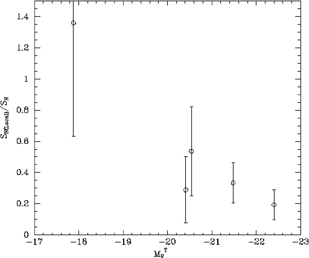
Figure 8: The ratio of S_N(Loc)/S_N vs the absolute magnitude of the host galaxy for the galaxies which have ground based measurements of the specific frequency. The local specific frequency is generally lower than the global value with a trend of decreasing S_N(Loc)/S_N with host luminosity (mass).

4 of the 5 galaxies which have ground based estimates of S_N all have smaller local specific frequency estimates in the inner regions than the global value. Furthermore, Fig 8 shows that the ratio of S_N(Local)/S_N increase as a function of the absolute magnitude of the host galaxy. This is consistent with other analyses of ellipticals (Forbes et al. 1996; Grillmair, Pritchet & van den Bergh 1986; Kundu et al. 1999) and S0s (Kundu & Whitmore 1998) that suggest that the globular cluster density distribution near the center of a galaxy is flatter than the stellar light distribution. Although NGC 3115 DW1 appears to be an exception in that the local specific frequency is larger than the global value, we point out that due to the small angular size of this dwarf the WFPC2 image likely subtends a large fraction ($\sim$80%) of both the galaxy light and cluster system of this host. Thus, we are effectively measuring the global specific frequency of NGC 3115 DW1. The difference between the effective global S_N calculated here and the smaller specific frequency reported in the literature may be due to larger statistical uncertainties in background subtraction in the earlier ground-based analysis. The roughly linear relationship between S_N(Local)/S_N and M${}_{V}^{T}$ is largely due to the fact that a larger fraction of the cluster system of smaller, less massive galaxies is subtended within the WFPC2 field-of-view. The elliptical sample in Paper I shows a similar effect. Thus, based on our analysis of the specific frequencies in the inner regions of ellipticals and S0s it is apparent that S0s are significantly less cluster rich than ellipticals.

4 Globular Cluster vs Host Galaxy Properties

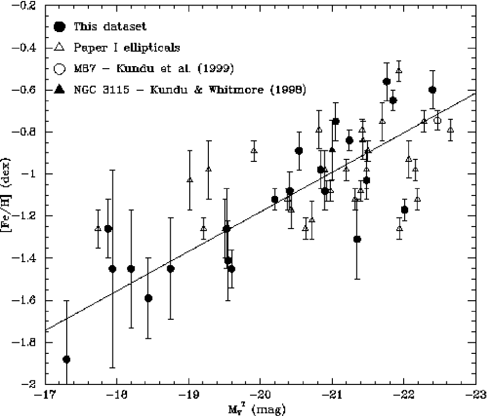
Figure 9: The average metallicity of the cluster systems vs the absolute magnitude of the host galaxy. Only S0 systems with N_bg/N_cand$<$0.25 have been plotted as these have reliable color estimates. The elliptical galaxies from Paper 1, M87 and NGC 3115 have also been plotted for comparison. The metallicity of the GCSs of S0s increases with host luminosity, consistent with the trend seen for ellipticals. The solid line traces the best fit straight line through the S0 data set.

Now that we have established the broad characteristics of the GCSs (Table 2) we turn to questions about their relationship with the parent galaxy and the implications on various formation and evolutionary scenarios. In Fig 9 we plot the average metallicity of the cluster systems (adopting the V-I to Fe/H transformation equation from Kundu & Whitmore 1998) vs the absolute magnitudes of the host galaxies. We have not plotted the values for GCSs with N_bg/N_cand $>$ 0.25 as the color estimates for these are likely to be affected by contaminating sources. The magnitudes plotted along the horizontal axis are not the values listed in Table 2 but the integrated magnitudes of the entire galaxy obtained from the NED catalog, normalized by the Table 1 distances. We have also included WFPC2 data points for NGC 3115 (Kundu & Whitmore 1998), the elliptical sample from Paper 1, and M87 (Kundu et al. 1999), all of which have V-I color measurements. At face value Fig 9 suggests that there is an overall tendency for brighter S0 galaxies to have more metal rich cluster systems.

The existence of the magnitude-mean metallicity relationship has been a rather contentious issue and there are conflicting reports in the literature. While van den Bergh (1975), Forbes et al. (1996) and Bridges et al. (1997) claim that the GCS metallicity-galaxy luminosity relationship is valid for all types of galaxies, Ashman & Bird (1993) suggest that elliptical galaxies show no perceptible trend. However, our analysis of ellipticals in Paper I, and Fig 9, confirm the existence of such a trend in both ellipticals and S0s, with no obvious offset between the two. A linear fit to only our S0 sample yields the expression.

[Fe/H] = -4.9($\pm$0.6) - 0.19($\pm$0.03) M${}_{V}^{T}$

The stars in the host galaxies themselves show a similar relationship between Fe/H and M${}_{V}^{T}$ (Brodie & Huchra 1991). The implied fact that the galaxy metallicity and the GC metallicity are correlated is not surprising in itself as it simply suggests that cluster formation is accompanied by star formation in the galaxy. Though neither the merger model nor the multiple collapse model explicitly predict such a relationship between the metallicity of the globular cluster distribution and the absolute magnitude (mass) of the host galaxy, it is not inconsistent with either model. The similar spread of S0 and elliptical GCS metallicities in Fig 9, and the almost identical mean metallicities of our S0 and elliptical samples do however suggest that the metallicity of the cluster system of an individual galaxy is primarily a function of the magnitude (mass) of the host galaxy and not of its Hubble type.

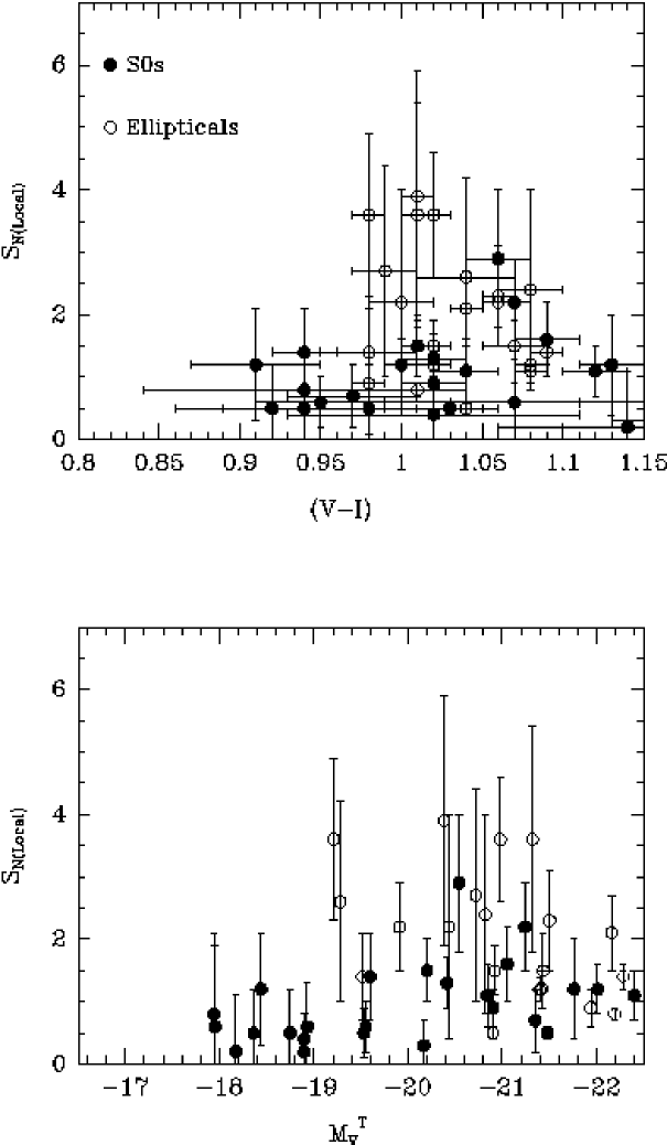
Figure 10: Top: The variation in the local specific frequency with mean color of the cluster system. Only systems with N_bg/N_cand$<$0.25 have been plotted as these have reliable color estimates. Elliptical galaxies from Paper I have also been shown. Bottom: The variation of the local specific frequency within our field of view with host galaxy brightness for the S0 sample from this paper and the elliptical galaxies from Paper I. Only elliptical candidates with $\delta$S_N $<$ 3 and S0s with $\delta$S_N $<$ 1.5 are plotted. As explained in the text the uncertainty in the local specific frequency of S0s is underestimated by a factor of 2 as compared to the ellipticals.

In the top panel of Fig 10 we plot the local specific frequency vs the mean color of the cluster system for the S0 and elliptical samples (restricted to S0 systems with $\delta$S_N(Local) $<$ 1.5 and elliptical systems with $\delta$S_N(Local) $<$ 3 for the reasons outlined in the previous section). There is no obvious trend in the local specific frequency of S0s with mean cluster color. Even for elliptical galaxies, in which the global specific frequencies have been shown to be weakly correlated with color (Ashman & Zepf 1998 and references therein), we see no obvious trend in the local specific frequencies. Thus, the local specific frequency which is sensitive to the field-of-view, and possibly the effects of destruction mechanisms in the inner regions of galaxies, is not very helpful in discerning the efficiency of cluster formation at various metallicities. Further studies of global specific frequencies are needed to establish whether metal-rich S0 systems are more cluster rich, and the impact of the results on the various models of S0 formation e.g. minor mergers (Schweizer 1990), multiple collapse (Forbes et al. 1996), or stripped spirals (Spitzer & Baade 1951; Gunn & Gott 1972).

In the bottom panel of Fig 10 the local specific frequency of S0s and ellipticals are plotted as a function of host magnitude. While there is no obvious trend in the elliptical or S0 samples individually, there is evidence that the local specific frequency of ellipticals at all host galaxy absolute magnitudes (masses) is slightly higher than that of S0s. This effect is more apparent for the less massive galaxies. For the most massive hosts a much smaller fraction of the total cluster system - and indeed of the galaxy - is visible within the HST field-of-view, and the local specific frequency may be influenced more by destruction effects than by global host galaxy morphology. Furthermore, considering the selection effect of the brightest galaxies in our sample(s) being spread out over a larger range of distances, coupled with the effects of calculating S_N within the fixed WFPC2 field-of-view, we do not consider the apparent lack of an offset in the local specific frequencies of the brightest ellipticals and S0s to be a very secure or significant result.

It is well known that specific frequency is a function of Hubble type; early type galaxies have richer globular cluster systems than later ones (Harris 1991). With our large sample of S0 galaxies we can attempt to check whether there are any trends within S0s. Preferably, one would like to define the position of a particular galaxy on the Hubble sequence using a quantitative estimator like the disk-to-bulge ratio. Unfortunately, the disk-to-bulge ratio has not been calculated for many of our galaxies, and it is not possible for us to determine it based on our own data due to the limited field-of-view. We attempted to bin the galaxies by their morphological classification in Table 1 but we soon discovered that some of the classifications were at odds with the structures seen in our images. We finally decided to roughly reclassify the objects ourselves after visually inspecting the images. We consider all galaxies which have star forming regions or obvious structure in the disk to be of S0⁺ type, galaxies that have a structureless disk to be of S0⁰ type; the remainder we classify as S0^-. Many of the S0^- galaxies may be more accurately classified as disky ellipticals, nevertheless we use the classification scheme outlined above for the purpose of this study. Fig 11 plots the variation of S_N(Local) as a function of galaxy type for systems with $\delta$S_N(Local) $<$ 1.5. While there is a statistically insignificant difference between the average specific frequencies of S0^- [1.03$\pm$0.7 (0.2)] and S0⁰ [0.95$\pm$0.6 (0.2)] galaxies, S0⁺s [0.7$\pm$0.4 (0.3)] appear to be significantly less cluster rich than than the early types. Hence, our observations are in agreement with the general trend that later type galaxies are less cluster-rich and suggest that the average specific frequency may vary smoothly across Hubble type. Finally, we note with interest that a significant fraction of S0s of all types actually have a genuinely low specific frequency. While much effort has been spent in trying to understand why certain galaxies have inordinately large values of S_N, the equally intriguing, but neglected problem of why some galaxies genuinely lack clusters might hold as many important clues to understanding the formation and evolution of cluster systems.

5 Globular Cluster System vs Galaxy Cluster Properties

There are indications that the properties of globular cluster systems may be correlated with the galaxy cluster that the host resides in. Blakeslee (1997) found that the number of globular clusters around the central galaxy in his sample of Abell clusters is proportional to the velocity dispersion (or mass) of the Abell cluster. There have also been suggestions that the specific frequency of clusters in a galaxy is linked to the position of the galaxy within the host cluster, with more centrally located galaxies having richer cluster systems.

Our (sample of) galaxies reside in widely disparate environments. Some of them are field galaxies, some are in poorly defined groups and others in well defined galaxy clusters. Although we cannot determine the position of the host galaxy within a cluster for most of our candidates as they are in poorly defined groups, we can attempt to define the total mass of the galaxy cluster system and look for correlations with GC properties. The mass of a galaxy cluster is usually best determined from the X-ray temperature. Unfortunately, very few of our sample galaxies reside in clusters that have X-ray temperatures (or any X-ray gas for that matter). Instead we use the number of bound galaxies in the host cluster of each program galaxy, as determined by the LGG classification of Garcia (1993) as an estimate of the mass of the host galaxy cluster. This is obviously not a very satisfying way of estimating the mass of the galaxy cluster but it allows us to very roughly differentiate small galaxy clusters from large one.

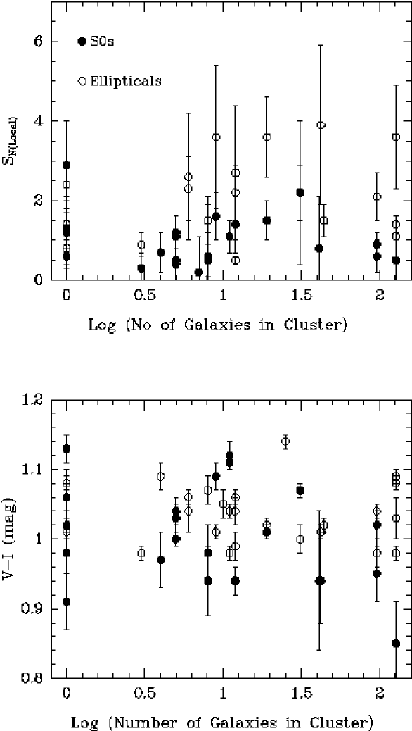
Figure 12: Top: The local specific frequencies of globular cluster systems in S0s and ellipticals (from Paper I) as a function of the log of the number of galaxies in the host galaxy cluster. The selection criteria for plotting a galaxy are the same as in Fig 10. Bottom: The average metallicity of the GCSs in ellipticals and S0s vs the log of the number of galaxies in the host galaxy cluster.

The local specific frequency and average color of the elliptical and S0 systems are plotted as a function of the logarithm of the number of galaxies in the host (galaxy) cluster in Fig 12. Note that the algorithm used by Garcia (1993) is sensitive to subclustering within large galaxy clusters like Virgo and Fornax, hence the number of galaxies in these clusters appear to be smaller than one would expect. There is no obvious trend in the specific frequency or color of the GCS with galaxy cluster properties. We also traced the positions of the galaxies in the Virgo and Fornax clusters on maps of the respective galaxy clusters to see if there is any correlation with position. While the complicated structure of the Virgo cluster makes the determination of its boundaries quite difficult, the Fornax cluster is much more compact and better defined. While NGC 1375 and NGC 1389 appear to be fairly close to the core of the Fornax cluster, IC 1919 and ESO 358-G034 lie on the outskirts of the cluster. The similar, low specific frequencies of all 4 galaxies reveal no correlation between the specific frequency and location within the cluster.

6 Sizes of the Clusters

As mentioned in $\S$2 the profiles of the globular clusters in our galaxy sample are slightly broader than stellar profiles, indicating that they are spatially resolved. Using the technique described in Kundu & Whitmore (1998) we measured the sizes of the clusters. The median half-light radius of the clusters in the PC, for galaxies that have at least five candidates in the chip, are listed in Table 4. The distance estimates from Table 1 have been used to convert the angular size to parsecs.

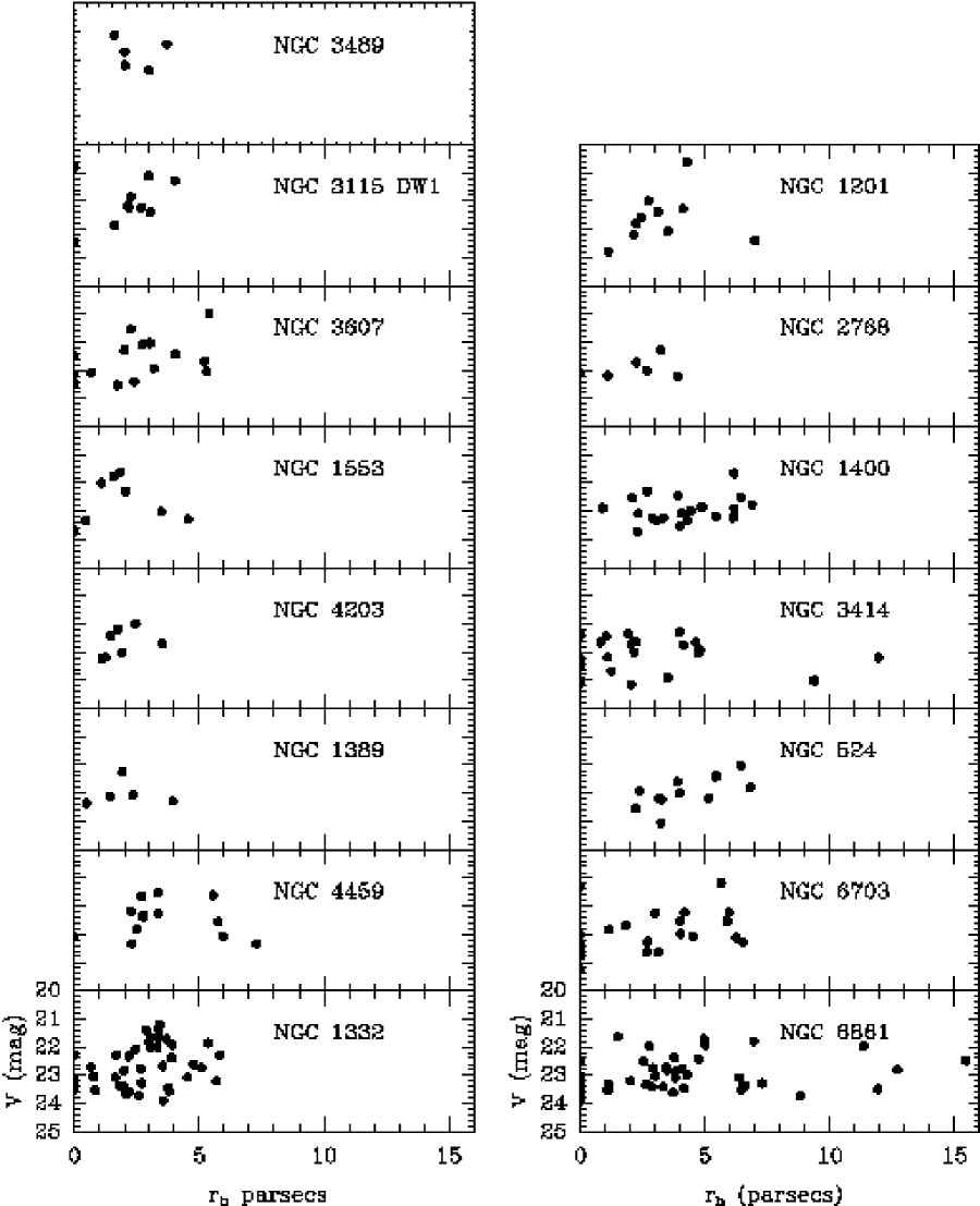
Figure 13: The half-light radius vs V-band magnitude of globular clusters in the PC. Only galaxies with at least 5 cluster candidates in the PC are plotted. The half light radii of clusters in all the galaxies largely fall in a narrow range of sizes between 0-7 pc. The half light radius does not appear to depend on the luminosity (mass) of the clusters.

The half-light radii (r_h) of individual clusters in the PC - using Table 1 distances - are plotted against cluster magnitudes for each of the galaxies in Fig 13. As in the elliptical sample in Paper I we find that the half light radius of clusters fall within a fairly narrow range of 0 - 6 pc in all cases with no apparent variation with magnitude. The large scatter in the sizes of the clusters in NGC 6861 is due to the fact that the S/N is the lowest in this the most distant galaxy of our sample. There is a small trend of increasing mean r_h with distance to the galaxy which, for the reasons outlined in Paper I, we suspect is due to small errors in the adopted PSF model. The mean half-light radius of our S0 sample is 2.6$\pm$0.7 (0.26), which is consistent with the 2.4$\pm$0.4 pc mean size of clusters in elliptical galaxies derived in Paper I and the 3 pc typical half-light radius of globular clusters in the Milky Way (van den Bergh 1996).

7 Summary

We have studied the cluster systems of 34 S0 galaxies from short exposure, ’snapshot’ WFPC2 images in the V (F555W) and I (F814W) bands. Of these 34 host galaxies, 29 have measurable globular cluster systems. In each galaxy we have detected a population of old globular clusters with colors in the range 0.5$<$V-I$<$1.5 mag.

The mean color (metallicity) of the GCSs of individual galaxies varies from V-I=0.85 mag ([Fe/H]=-1.88 dex) to V-I=1.17 mag ([Fe/H]=-0.37 dex). The average metallicity of S0 GCSs is [Fe/H]=-1.1$\pm$0.3 dex (V-I=1.00$\pm$0.07 mag) which is very similar to that derived for ellipticals in Paper I [Fe/H]=-1.0$\pm$0.2 dex. The mean metallicity of the cluster system of both S0s and ellipticals appears to be primarily a function of the absolute magnitude (mass) of the host galaxy with no apparent dependence on the Hubble type.

On the other hand, the local specific frequency of S0s is smaller than that of ellipticals. The mean S_N(Local) for S0s, 1.0$\pm$0.6 (0.1) is significantly smaller than the value of S_N(Local) = 2.4$\pm$1.8 (0.4) derived for ellipticals in Paper I. The local frequencies of very late type S0 galaxies (S0⁺) is statistically lower than that of early types (S0^- and S0⁰) which further suggests that the mean specific frequency is a function of Hubble type.

Although NGC 2768 is the only galaxy in our sample with a confirmed bimodal metallicity distribution statistical tests indicate that several other galaxies are promising candidates for bimodality e.g. NGC 1332 and NGC 1553. Including S0 galaxies previously studied, we estimate that at least 10$\%$-20$\%$ of S0 galaxies have bimodal cluster distributions at the present level of photometric uncertainty.

The average half light radius of globular clusters in S0 galaxies is 2.6$\pm$0.7 pc. which is similar to that of ellipticals (Paper I) and the Milky Way.

There are no significant trends in the mean metallicities or specific frequency of GCSs with membership of the host in a galaxy cluster. We also find no evidence of a dependence of globular cluster properties with the location of the host within the galaxy cluster.

For the richest few S0 systems for which we derived the turnover luminosity, the GCLF distances were in good agreement with other estimates. As in the elliptical sample we find evidence that the difference in the turnover luminosities in V and I increases with metallicity. In Paper I we found that the GCLF turnover magnitude of ellipticals is an excellent distance indicator with an accuracy comparable with the surface brightness fluctuation method ($\sim$0.1mag). There is every likelihood that deeper images of S0s, and more accurate comparative distance estimates using other indicators, will reveal a similar level of confidence in the use of S0 GCLFs as distance indicators.

AK is grateful to Mike A’ Hearn, Francois Schweizer, Sylvain Veilleux and Stuart Vogel for numerous suggestions that helped improve this paper in its earlier incarnation as a chapter of his thesis. Yan Fernandez for all his suggestions and help. The authors would also like to thank the referee Doug Geisler for his useful comments and suggestions. Support for this work was provided by NASA through grant number AR-08378.01-97A from the Space Telescope Science Institute, which is operated by AURA, Inc., under NASA contract NAS5-26555. This research has made use of the NASA/IPAC Extragalactic Database (NED) which is operated by the Jet Propulsion Laboratory, California Institute of Technology, under contract with the National Aeronautics and Space Administration.

Figure 11: The variation of the local specific frequency with Hubble type (see text for details of our binning parameters). The positions of the points have been shifted by arbitrary small amounts along the abscissa to help distinguish individual data points. Only candidates with $\delta$S_N $<$ 1.5 are plotted. There is a weak trend of later type S0s having lower specific frequencies.

Table 1: General Properties of the Program Galaxies

Galaxy	Morph. Typ	Gp/Clstr	Hel. Vel	Dist	AV	M${}_{V}^{T^{0}}$
			Km s-1	Mpc	mag	mag
(1)	(2)	(3)	(4)	(5)	(6)	(7)
NGC 524	SA(rs)0+	NGC 524Gp	2421	32.6	0.10	-22.4
NGC 2768	S01/2/E6,LIN	NGC 2768Gp	1339	22.8	0.12	-22.0
NGC 6861	SA(s)0-	Telescopium	2819	36.6	0.11	-21.8
NGC 6703	SA0-		2365	36.6	0.20	-21.8
NGC 1553	SA(rl)00,LIN	Dorado	1080	14.9	0.0	-21.5
NGC 474	(R′)SA(s)00	NGC 488Gp	2372	31.6	0.04	-21.4
NGC 1332	S(s)0-:sp	Eridanus	1524	20.0	0.02	-21.2
NGC 3414	S0 pec	LGG 227	1414	24.5	0.0	-21.0
NGC 4459	SA(r)0+	Virgo I	1210	17.3†	0.06	-20.9
NGC 1201	SA(r)00	NGC 1255Gp	1671	20.5	0.0	-20.8
NGC 1400	SA0-	Eridanus A	558	22.9†	0.10	-20.6
NGC 3607	SA(s)00	Leo II	935	11.4	0.0	-20.4
NGC 4203	SAB0-,LIN	Coma I	1086	15.0	0.0	-20.2
NGC 2902	SA(s)00	LGG 174	1990	27.4	0.19	-20.2
NGC 3489	SAB(rs)0+	Leo I	708	9.7	0.02	-19.6
NGC 4379	S0- pec:	Virgo I	1069	17.3†	0.02	-19.6
NGC 1389	SAB(s)0-	Fornax	986	16.4	0.0	-19.5
NGC 3056	SA(rl)00		1017	12.4	0.12	-18.9
NGC 3156	S0	NGC 3166Gp	1118	16.3	0.03	-18.9
IC 3131	d:S01(0),N:	Virgo W′?	1596	30.0†	0.0	-18.9‡
NGC 1375	SAB00:sp	Fornax	740	16.4	0.0	-18.8
VCC 165	S01(0,2):	Virgo M?	255	30.0†	0.02	-18.5‡
NGC 3599	SA0	Leo II	781	11.4	0.0	-18.4
NGC 2328	(R′)SAB0-		1159	13.5	0.33	-18.4
NGC 4431	SA(r)0	Virgo I	913	17.3†	0.06	-18.4
IC 1919	SA(rs)0-?	Fornax	1220	16.4	0.0	-18.2‡
NGC 1581	S0-	Dorado	1600	14.9	0.0	-18.2
ESO 358- G 059	SAB0-	Fornax	1007	16.4	0.0	-18.0
NGC 3870	S0?	U Ma NED3	756	15.5	0.0	-17.9
NGC 3115 DW1	SA(s)00 pec		715	11.0	0.13	-17.9
ESO 118- G 034	S00 pec	NGC 1672Gp	1178	13.3	0.0	-17.6
IC 3540	SB0	Virgo I	753	17.3†	0.08	-17.3‡
NGC 4150	SA(r)00?	C Vn I	226	4.3†	0.03	-16.6
NGC 404	SA(s)0-	LGG 11	-48	3†	0.17	-16.5

cllllllll 2 Globular Cluster Properties
Galaxy & $<$V-I$>$ [Fe/H] N_cand N_bg N_Tot M${}_{V}^{FOV}$ S_N(Local) S_N^‡
mag dex mag
(1) (2) (3) (4) (5) (6) (7) (8) (9)
NGC 524 1.12 (0.02) -0.6 (0.09) 113 9 645 -21.9 1.1$\pm$0.4 5.7$\pm$1.8
NGC 2768 1. (0.01) -1.17 (0.05) 118 6 343 -21.2 1.2$\pm$0.4
NGC 6861 1.11 (0.01) -0.65 (0.05) 235 25 1858 -21.8 3.6$\pm$1.6
NGC 6703 1.13 (0.02) -0.56 (0.09) 82 16 560 -21.7 1.2$\pm$0.8
NGC 1553 1.03 (0.02) -1.03 (0.09) 70 7 114 -21. 0.5$\pm$0.1 1.5$\pm$0.5
NGC 474 0.97 (0.04) -1.31 (0.19) 34 2 185 -21. 0.7$\pm$0.5
NGC 1332 1.07 (0.01) -0.84 (0.05) 204 10 501 -20.9 2.2$\pm$0.7
NGC 3414 1.09 (0.02) -0.75 (0.09) 117 4 397 -21. 1.6$\pm$0.6
NGC 4459 1.02 (0.02) -1.08 (0.09) 75 3 148 -20.6 0.9$\pm$0.3
NGC 1201 1.04 (0.02) -0.98 (0.09) 77 9 177 -20.5 1.1$\pm$0.5
NGC 1400 1.06 (0.02) -0.89 (0.09) 158 3 419 -20.4 2.9$\pm$1.1 5.4$\pm$2
NGC 3607 1.02 (0.02) -1.08 (0.09) 98 6 130 -20. 1.3$\pm$0.4 4.5$\pm$3
NGC 4203 1.01 (0.01) -1.12 (0.05) 106 5 175 -20.2 1.5$\pm$0.5
NGC 2902 1.17 (0.04) -0.37 (0.19) 15 5 35 -20.2 0.3$\pm$0.4
NGC 3489 0.94 (0.02) -1.45 (0.09) 46 4 51 -18.9 1.4$\pm$0.7
NGC 4379 0.95 (0.04) -1.41 (0.19) 22 3 37 -19.6 0.6$\pm$0.4
NGC 1389 0.98 (0.04) -1.26 (0.19) 19 2 32 -19.5 0.5$\pm$0.4
NGC 3056 1.07 (0.04) -0.84 (0.19) 25 8 23 -18.9 0.6$\pm$0.7
NGC 3156 1.02 (0.09) -1.08 (0.42) 11 3 13 -18.9 0.4$\pm$0.4
IC 3131 3 1 8 -18.9 0.2$\pm$0.4
NGC 1375 0.94 (0.05) -1.45 (0.24) 11 1 17 -18.7 0.5$\pm$0.7
VCC 165 11 6 0 -18.5 0.$\pm$2.1
NGC 3599 0.91 (0.04) -1.59 (0.19) 21 1 29 -18.4 1.2$\pm$0.9
NGC 2328 18 13 0 -18.4 0.$\pm$1.4
NGC 4431 0.92 (0.06) -1.55 (0.28) 10 2 11 -18.4 0.5$\pm$0.7
IC 1919 0.94 (0.06) -1.45 (0.28) 13 2 21 -18.2 1.1$\pm$1.7
NGC 1581 1.14 (0.08) -0.51 (0.38) 8 5 4 -18.2 0.2$\pm$0.9
ESO 358-G059 1.07 (0.09) -0.84 (0.42) 7 2 9 -17.9 0.6$\pm$1.3
NGC 3870 0.94 (0.1) -1.45 (0.47) 8 1 13 -17.9 0.8$\pm$1.3
NGC 3115 DW1 0.98 (0.03) -1.26 (0.14) 37 5 42 -17. 6.8$\pm$2.4 5$\pm$2
ESO 118-G034 9 6 3 -17.6 0.3$\pm$2.
IC 3540 0.85 (0.06) -1.88 (0.28) 14 1 26 -17.3 3.2$\pm$4.2
NGC 4150 0.92 (0.06) -1.55 (0.28) 10 2 7 -16.6 1.7$\pm$1.8
NGC 404 83 48
Avg^b 1.00$\pm$0.07^a -1.1$\pm$0.3^a 1.0$\pm$0.6^†
1 Galaxy Name; 2 V-I color in mag; 3 [Fe/H] in dex; 4 No of candidate objects in the color range 0.5$<$V-I$<$1.5 ; 5 No of objects with colors in the the range 0.0$<$V-I$<$0.5 or 1.5$<$V-I$<$2.0; 6 Calculated total number of globular clusters in the field of view; 7 Total V band luminosity of the galaxy within the field of view; 8 The local Specific Frequency of globular clusters; 9 Global Specific Frequency from the compilation of Kissler-Patig (1997) and references therein. † Avg S_N(Loc) of systems with $\delta$S_N(Loc) $<$ 1.5 ‡ The values of S_N have been adjusted to Table 1 distances. a Only systems with N_bg/N_cand $<$ 0.25 have been considered in the calculation of the mean colors and metallicities. b The average color, metallicity and specific frequency, and associated uncertainties, are unchanged by the addition of the NGC 4550 values from Paper 1.

llllllll 3 Distances from the GCLF
Galaxy & m${}_{V}^{0}$ m${}_{I}^{0}$ (m-M)_Vel (m-M)_Lit (m-M)_V^† (m-M)_I^† $<$m-M$>_{GCLF}$^†
(1) (2) (3) (4) (5) (6) (7) (8)
NGC 3489 22.69$\pm$0.11 21.94$\pm$0.14 29.9 30. 30.1$\pm$0.1 30.4$\pm$0.1 30.25$\pm$0.09
NGC 3115 DW1 22.48$\pm$0.07 21.64$\pm$0.12 30.2 29.89$\pm$0.08 30.1$\pm$0.1 30.$\pm$0.07
NGC 3607 24.07$\pm$0.33 23.04$\pm$0.3 30.3 31.5 31.48$\pm$0.3 31.5$\pm$0.3 31.49$\pm$0.22
NGC 1553 25.15$\pm$0.65 23.89$\pm$0.84 30.9 30.8
NGC 4203 23.05$\pm$0.13 22.05$\pm$0.14 30.9 30.46$\pm$0.1 30.51$\pm$0.1 30.49$\pm$0.10
NGC 4459 23.98$\pm$0.27 23.73$\pm$0.63 31.2 30.9
NGC 1400 24.94$\pm$0.43 23.74$\pm$0.39 31.5 31.9 32.35$\pm$0.4 32.2$\pm$0.4 32.28$\pm$0.29
NGC 1332 24.34$\pm$0.35 23.19$\pm$0.32 31.5 31.5 31.75$\pm$0.4 31.65$\pm$0.3 31.7$\pm$0.24
NGC 1201 24.95$\pm$0.63 23.91$\pm$0.46 31.6
NGC 2768 24.2$\pm$0.28 23.06$\pm$0.33 31.8 31.6 31.61$\pm$0.3 31.52$\pm$0.3 31.57$\pm$0.22
NGC 3414 24.85$\pm$0.53 23.89$\pm$0.64 31.9 31.8
NGC 524 24.97$\pm$0.39 24.15$\pm$0.48 32.6
NGC 6703 24.34$\pm$0.34 23.18$\pm$0.32 32.8 32.4 31.75$\pm$0.3 31.64$\pm$0.3 31.70$\pm$0.23
NGC 6861 25.05$\pm$0.48 24.$\pm$0.47 32.8

1 Galaxy Name; 2 GCLF V-band turnover; 3 GCLF I-band turnover; 4 Distance modulus from recessional velocity; 5 Distance modulus from the literature. See text for details ; 6 Distance modulus from V Band GCLF; 7 Distance modulus from I band GCLF; 8 Mean distance modulus from V and I band GCLFs † GCLF distances are reported only for those galaxies with uncertainty in the mean GCLF distance less than 0.3 mag.

llll 4 Cluster Sizes in the PC
Galaxy & Number r_h
in PC $pc$
1 2 3
NGC 3489 5 2.0
NGC 3115 DW1 10 2.2
NGC 3607 15 2.4
NGC 1553 8 1.7
NGC 4203 8 1.7
NGC 1389 5 1.9
NGC 4459 13 2.8
NGC 1332 41 3.0
NGC 1201 10 2.9
NGC 2768 6 2.5
NGC 1400 21 4.0
NGC 3414 24 2.0
NGC 524 11 3.9
NGC 6703 23 2.7
NGC 6861 46 3.4
Avg 2.6$\pm$0.7 (0.26)

1 Galaxy; 2 Number of cluster candidates in the PC chip; 3 Median half-light radius in parsecs.

References

- [1] Ashman, K. M., & Bird, C. M. 1993, AJ, 106, 2281
- [2] Ashman, K. M., Bird, C. M., & Zepf, S. E. 1994, AJ, 108, 2348
- [3] Ashman, K. M., Conti, A., & Zepf, S. E. 1995, AJ, 110, 1164
- [4] Ashman, K. M., & Zepf, S. E. 1992, ApJ, 384, 50
- [5] Ashman, K. M., & Zepf, S. E. 1998, Globular Cluster Systems (Cambridge: Cambridge University Press)
- [6] Bingelli, B., Sandage, A. & Tammann, G. A. 1985, AJ, 90, 168
- [7] Blakeslee, J. P. 1997, ApJ, 481, L59
- [8] Bridges, T. J., Ashman, K. M., Zepf, S. E., Carter, D., Hanes, D. A., Sharples, R. M., & Kavelaars, J. J. 1997, MNRAS, 284, 376
- [9] Brodie, J. P., & Huchra, J. 1991, ApJ, 379, 157
- [10] Bruzual, A., & Charlot, S. 1993, ApJ, 405, 538
- [11] Burstein, D., & Heiles, C., 1982, AJ, 87, 1165
- [12] Durrell, P. R., McLaughlin, D. E., Harris, W. E., & Hanes, D. A. 1996, ApJ, 463, 543
- [13] Forbes, D. A., Brodie, J. P., Grillmair, C. J. 1997, AJ, 113, 1652
- [14] Forbes, D. A., Franx, M., Illingworth, G. D., & Carollo, C. M. 1996, ApJ, 467, 126
- [15] Fouque, P., Gourgoulhon, E., Chamaraux, P., & Paturel, G. 1992, A&AS, 93, 211
- [16] Garcia, A. M. 1993, A&AS, 100, 47
- [17] Geller, M. J., & Huchra, J. P. 1983, ApJS, 52, 61
- [18] Grillmair, C., Pritchet, C., & van den Bergh, S. 1986, AJ, 91, 1328
- [19] Gunn, J. E., & Gott, J. R. 1972, ApJ, 176, 1
- [20] Hanes, D. A., & Harris, W. E. 1986, ApJ, 304, 599
- [21] Harris, W. E. 1991, ARA&A, 29, 543
- [22] Harris, W. E., & van den Bergh, S. 1981, AJ, 86, 1627
- [23] Holtzman, J. et al. (the WFPC2 team) 1995a PASP, 107, 156
- [24] Holtzman, J. et al. (the WFPC2 team) 1995b PASP, 107, 1065
- [25] HST Data Handbook, 1997, Space Telescope Science Institute, Baltimore
- [26] Huchra, J. P., & Geller, M. J. 1982, ApJ, 257, 423
- [27] Jacoby, G. H. et al. 1992, PASP, 104, 599
- [28] Jensen, J. B., Tonry, J. L., & Luppino, G. A. 1998, ApJ, 505, 111
- [29] Kissler-Patig, M., Richtler, T., Storm, J. & Della Valle, M. 1997, A&A, 327, 503
- [30] Kundu, A., & Whitmore, B. C. 1998, AJ, 116, 2841
- [31] Kundu, A., & Whitmore, B. C. 2001, AJ, submitted (Paper I)
- [32] Kundu, A., Whitmore, B. C., Sparks, W. B., Macchetto, F. D., Zepf, S. E., & Ashman, K. M. 1999, ApJ, 513, 733
- [33] Lee, M. G., Freedman, W., & Madore, B. F. 1993, ApJ, 417, 553
- [34] Makarova, L., Karachentsev, I., Takalo, L. O., Heinaemaeki, P., & Valtonen, M. 1998, A&AS, 128, 459
- [35] Mathis, J. S. 1990, ARA&A, 28, 37
- [36] NED, The NASA/IPAC Extragalactic Database, The NASA/IPAC Extragalactic Database is operated by the Jet Propulsion Laboratory, California, Institute of Technology, under contract with the National Aeronautics and Space Administration.
- [37] Persson, S. E., Frogel, J. A., & Aaronson, A. 1979, 39, 61
- [38] Postman, M., & Lauer, T. R. 1995, ApJ, 440, 28
- [39] Prugniel, P., & Simien, F. 1996, A&A, 309, 749
- [40] Puzia, T. H., Kissler-Patig, M., Brodie, J. P., & Schroder, L. L. 2000, AJ, 120, 777
- [41] Sandage, A. 1975, ApJ, 202, 563
- [42] Sandage, A., & Visvanathan, N. 1978, ApJ, 223, 707
- [43] Schweizer, F. 1987, in Nearly Normal Galaxies, ed. S. Faber (New York: Springer)p. 18
- [44] Schweizer, F. 1990, in Dynamics and Interaction of Galaxies, ed. R. Wielen (Berlin: Springer-Verlag)p. 60
- [45] Secker, J. 1992, AJ, 104, 1472
- [46] Spitzer, L., & Baade, W. 1951, ApJ, 113, 413
- [47] van den Bergh, S. 1975, ARA&A, 13, 217
- [48] van den Bergh, V. 1996, AJ, 112, 2634
- [49] Whitmore, B. C. 1996, in The Extragalactic Distance Scale, Proceedings of the STScI May Symposium, held in Baltimore, MD, May 7-10 1996,
- [50] eds. M. Livio, M. Donahue, and N. Panagia ( Cambridge: Cambridge University Press), p. 254
- [51] Whitmore, B. C., & Heyer I. 1997, WFPC2 Instrument Science report 97-08, ”New results on charge transfer efficiency and constraints on the flat-field accuracy”
- [52] Whitmore, B. C., Heyer, I., & Casertano, S. 1999, PASP, 111, 1559
- [53] Wiklind, T., & Henkel, C. 1990, A&A, 227, 394
- [54] Worthey, G. 1994, ApJS, 95, 107
- [55] Zepf, S. E., & Ashman, K. M. 1993, MNRAS, 264, 611
- [56]