Cold Dark Matter and Strong Gravitational Lensing:
Concord or Conflict?

Abstract

Using the number and sizes of observed gravitational lenses, I derive upper limits on the dark matter content of elliptical galaxies. On average, dark matter can account for no more than 33% of the total mass within one effective radius ($R_{e}$) of elliptical galaxies, or 40% of the mass within $2R_{e}$ (95% confidence upper limits). I show that galaxies built from Cold Dark Matter (CDM) mass distributions are too concentrated to comfortably satisfy these limits; a high-density ($\Omega_{M}=1$) CDM cosmology is ruled out at better than 95% confidence, while a low-density, flat cosmology is only marginally consistent with the lens data. Thus, lensing adds to the evidence from spiral galaxy dynamics that CDM mass distributions are too concentrated on kiloparsec scales to agree with real galaxies, and extends the argument to elliptical galaxies.

Lensing also provides a unique probe of the very inner regions of galaxies, because images are predicted to form near the centers of lens galaxies but are not observed. The lack of central images in deep maps of radio lenses places strong lower limits on the central densities of galaxies. The central densities of CDM galaxies are too low on $\sim$10 parsec scales. Supermassive black holes can help suppress central images, but they must lie well off the observed black hole–bulge mass correlation in order to satisfy current limits on central images. Self-interacting dark matter, or any other modification to regular cold dark matter, must simultaneously reduce the densities on kiloparsec scales and increase the densities on parsec scales in order to satisfy the unique constraints from lensing.

1 Introduction

Cuspy mass distributions are a robust prediction of the popular Cold Dark Matter (CDM) paradigm. Numerical simulations of collisionless cold dark matter predict density profiles with $\rho\propto r^{-\alpha}$ and $\alpha\simeq 1.0$–1.5 at small radii (e.g., Navarro, Frenk & White 1996, 1997; Moore et al. 1998, 1999; Jing & Suto 2000; Klypin et al. 2000), and this prediction does not depend on particular cosmogonies or initial conditions (Huss, Jain & Steinmetz 1999a, 1999b) or on the specific form of the dark matter power spectrum (Eke, Navarro & Steinmetz 2000). Adding dissipative baryons makes mass distributions even more concentrated (e.g., Blumenthal et al. 1986; Dubinski 1994). It is important to compare the predicted mass distributions with real galaxies to test the CDM paradigm as the explanation for the formation and growth of structure in the universe.

The dynamics of spiral galaxies have provided the most extensive observational tests of CDM. Salucci (2001; also see Salucci & Burkert 2000, and references therein) suggests that normal spiral galaxies have dark matter halos with large constant-density cores as opposed to cusps. Debattista & Sellwood (1998) and Weiner, Sellwood & Williams (2001) argue that fast-rotating bars require dark matter densities lower than predicted by CDM. The slowly-rising rotation curves of dwarf galaxies and low surface brightness galaxies also seem to imply constant-density cores (e.g., Flores & Primack 1994; Moore 1994; McGaugh & de Blok 1998; Blais-Ouellette, Amram & Carignan 2001; de Blok et al. 2001). However, several authors have argued that the Hi rotation curves may have appeared artificially shallow due to beam smearing, and that better data are actually consistent with cuspy CDM mass distributions (van den Bosch et al. 2000; van den Bosch & Swaters 2000; Swaters, Madore & Trewhella 2000). In rebuttal, McGaugh & de Blok (1998) and de Blok et al. (2001) claim that beam smearing does not affect their conclusions; and Moore (2001) argues that only two of the 19 galaxies analyzed by van den Bosch & Swaters (2000) are actually consistent with CDM. To summarize, many argue that CDM mass distributions are too concentrated to agree with the dynamics of spiral galaxies, but the conclusions are still subject to some vigorous debate.

Other tests of CDM mass distributions should not be affected by beam smearing. Navarro & Steinmetz (2000) and Eke et al. (2000) consider the global dynamical properties of spiral galaxies in terms of the Tully–Fisher (TF) relation between luminosity and circular velocity. They find that CDM can reproduce the slope and scatter of the TF relation, but has some trouble with the zero point. In a high-density ($\Omega_{M}=1$) cosmology, CDM model galaxies are too concentrated to agree with the TF zero point, while in a low-density cosmology the models are marginally consistent with the data. Taking an entirely different approach, Rix et al. (1997) study the line-of-sight velocity profile of the elliptical galaxy NGC 2434 using detailed dynamical models. They find that the galaxy is consistent with CDM models, but the strength of the conclusion is limited by systematic uncertainties such as the orbital anisotropy. These tests do not indicate a fundamental problem with CDM mass distributions, but they do not strongly favor the CDM models, either.

The dynamical tests are fundamentally limited by the need to interpret data from luminosity distributions before drawing conclusions about mass distributions. Given the importance of the CDM paradigm in modern cosmology, it is desirable to develop additional tests that are independent of, and hopefully less ambiguous than, the dynamical tests. One excellent possibility is gravitational lensing, because it offers a direct probe of mass distributions. Individual gravitational lenses robustly determine the masses of individual galaxies, and the statistical properties of the lens sample constrain properties of the galaxy population (e.g., Maoz & Rix 1993; Kochanek 1993, 1995, 1996; Cohn et al. 2001). Individual lenses and lens statistics both imply that elliptical galaxies (which dominate the mass-selected sample of lens galaxies; e.g., Kochanek et al. 2000) have approximately isothermal mass distributions out to several kiloparsecs, in agreement with the evidence from dynamics (e.g., Rix et al. 1997) and X-ray elliptical galaxies (e.g., Fabbiano 1989).

It is not clear whether the mass distributions implied by lensing are consistent with the predictions of CDM. Most lensing studies, even those that consider a wide range of density profiles (e.g., Kochanek 1995; Barkana 1998; Chae, Khersonsky & Turnshek 1998; Cohn et al. 2001; Muñoz, Kochanek & Keeton 2001), consider only single-component mass models. However, lens galaxies are likely to have at least two components (a stellar galaxy and a dark matter halo), which may contribute comparable amounts of mass (e.g., Rix et al. 1997). Both components are necessary to explain the distribution of lensed image separations and the fact that galaxies are much better lenses than more massive groups of galaxies (Keeton 1998; Porciani & Madau 2000; Kochanek & White 2001). Only by allowing two components can we use lensing to directly test whether real galaxies are consistent with CDM mass distributions.

The goal of this paper is to use two-component star+halo models for lensing to test the CDM paradigm. The focus is on elliptical galaxies because they dominate lens statistics. The outline of the paper is as follows. Section 2 defines the models, and Section 3 reviews the lensing calculations. In Section 4, the observed number and sizes of lenses are used to evaluate the global properties of the models. In Section 5, lensing is used to examine the very inner regions of galaxies. Finally, Section 6 offers a discussion and conclusions.

2 Star+Halo Models

This section defines star+halo models for elliptical galaxies in the context of the CDM paradigm. Section 2.1 discusses models for the stellar and dark matter components, and Section 2.2 gives normalizations for the models. Only spherical models are considered, because they are sufficient for calculations of the number and sizes of lenses. Departures from spherical symmetry mainly affect the relative numbers of 2-image and 4-image lenses (see Keeton, Kochanek & Seljak 1997; Rusin & Tegmark 2001).

2.1 Model components

A simple model for the stellar components of elliptical galaxies is the Hernquist (1990) model, which has a density profile

$$\rho(r)={\rho_{s}\over{(r/r_{s})(1+r/r_{s})^{3}}}\ .$$ (1)

This profile is described by a scale radius $r_{s}$, but the projected profiles of elliptical galaxies are usually described by an effective (or half-mass) radius $R_{e}$; they are related by $r_{s}=0.551R_{e}$. The total mass of a Hernquist model is $M=2\pi\rho_{s}r_{s}^{3}$. The projected surface mass density, in units of the critical density for lensing, is

$$\kappa(R)={\Sigma(R)\over\Sigma_{cr}}=\kappa_{s}\,{(2+x^{2}){\cal F}(x)-3\over(x^{2}-1)^{2}}\ ,$$ (2)

where $x=R/r_{s}$, $\kappa_{s}=\rho_{s}\,r_{s}/\Sigma_{cr}$, and the function ${\cal F}(x)$ is:

$${\cal F}(x)=\cases{{1\over\sqrt{x^{2}-1}}\,\mbox{tan}^{-1}\sqrt{x^{2}-1}&$(x>1)$\cr{1\over\sqrt{1-x^{2}}}\,\mbox{tanh}^{-1}\sqrt{1-x^{2}}&$(x<1)$\cr 1&$(x=1)$\cr}$$ (3)

The critical density is $\Sigma_{cr}=(c^{2}D_{s})/(4\pi GD_{l}D_{ls})$ where $D_{l}$ and $D_{s}$ are angular diameter distances to the lens and source, respectively, and $D_{ls}$ is the angular diameter distance from the lens to the source (e.g., Schneider, Ehlers & Falco 1992). The gravitational deflection for a Hernquist model is (see eq. 14 below)

$$\phi_{R}(R)=2\,\kappa_{s}\,r_{s}\,{{x[1-{\cal F}(x)]}\over{x^{2}-1}}\ .$$ (4)

Navarro, Frenk & White (1996, 1997, hereafter NFW) have argued that dark matter halos found in cosmological $N$-body simulation of collisionless dark matter have a “universal” density profile of the form

$$\rho(r)={\rho_{s}\over{(r/r_{s})(1+r/r_{s})^{2}}}\ ,$$ (5)

where $r_{s}$ is a scale radius and $\rho_{s}$ is a characteristic density. It is convenient to replace the scale radius with a “concentration” parameter $C=r_{200}/r_{s}$, where $r_{200}$ is the radius within which the mean density of the halo is 200 times the critical density of the universe, which is often taken to mark the boundary of a relaxed halo (e.g., Crone, Evrard & Richstone 1994; Cole & Lacey 1996; Navarro et al. 1996, 1997). The characteristic density is then

$$\rho_{s}={200\over 3}\,\rho_{crit}(z)\,{C^{3}\over{\ln(1+C)-C/(1+C)}}\ ,$$ (6)

where $\rho_{crit}(z)$ is the critical density of the universe at the redshift of the halo. The lensing properties of an NFW model are given by Bartelmann (1996).

More recently, Moore et al. (1998, 1999; also see Jing & Suto 2000; Klypin et al. 2000) have argued that the central regions of simulated halos are steeper than the NFW profile. They advocate a density of the form

$$\rho(r)={\rho_{s}\over{(r/r_{s})^{1.5}[1+(r/r_{s})^{1.5}]}}\ .$$ (7)

For Moore halos, I define a concentration parameter $C=r_{200}/r_{(-2)}$ in terms of the radius $r_{(-2)}$ at which the logarithmic slope of the density is $-2$. This definition is equivalent to the definition of the concentration for NFW halos, and Keeton & Madau (2001; also see Wyithe, Turner & Spergel 2000) argue that it is the best generalization of the concentration. The radius $r_{(-2)}$ is related to the scale radius $r_{s}$ in eq. (7) by $r_{(-2)}=0.630r_{s}$. The characteristic density of a Moore halo is

$$\rho_{s}=25\,\rho_{crit}(z)\,{C^{3}\over\ln[1+C^{3/2}/2]}\ .$$ (8)

Figure 1: Rotation curves for sample star+halo models with NFW halos. Each panel has the specified values of the concentration $C$ of the initial halo and the cooled mass fraction $f_{cool}$; all models have $R_{e}/r_{200}=0.03$. The solid curves show the total rotation curves, while the dotted and dashed curves show the contributions from the galaxy and halo, respectively. For comparison, the long dashed curves show the rotation curves of the initial NFW halos before adiabatic contraction. The velocities are scaled by the peak velocity of the galaxy component.

The dark matter halo models were derived from studies of collisionless dark matter. They do not hold in the presence of dissipative baryons, because as the baryons cool and condense into a galaxy they modify the gravitational potential and thus the dark matter distribution (e.g., Blumenthal et al. 1986; Dubinski 1994). Fortunately, there is a simple analytic prescription called adiabatic contraction for computing the changes to the dark matter distribution; it seems to agree well with gasdynamical simulations (e.g., Blumenthal et al. 1986; Flores et al. 1993), even for merger scenarios thought to produce elliptical galaxies (Gottbrath 2000). Appendix A gives an analytic solution for adiabatic contraction of an arbitrary dark matter halo by a Hernquist galaxy. Adiabatic contraction depends on the mass ratio of the cooled galaxy component to the total virial mass, $f_{cool}=M_{gal}/M_{tot}$, which is presumably no larger than the global baryon fraction of the system, $f_{bar}=M_{bar}/M_{tot}=\Omega_{b}/\Omega_{M}$. (There may be baryons that remain hot and distributed throughout the halo, so $f_{cool}\leq f_{bar}$.) The virial mass and radius of the system factor out to provide overall scalings, so the solution also depends on the fraction $f_{cool}$ of the concentration $C$ of the initial halo, and the effective radius of the galaxy (specifically $R_{e}/r_{200}$).

To illustrate the star+halo models, Figure 1 shows rotation curves for various values of the parameters. For a fixed stellar component, decreasing $f_{cool}$ increases the total mass of the halo ($M_{tot}=f_{cool}^{-1}\times M_{gal}$), which raises the rotation curve. Increasing the concentration of the initial halo packs more of the dark matter into the inner regions of the system, which also raises the inner rotation curve. In other words, changing either parameter affects the amount of mass contained within a few effective radii of the galaxy. Lensing can distinguish between the two parameters only if it is sensitive to the detailed shape of the galaxy mass profile inside a few $R_{e}$.

Figure 1 offers two important qualitative results. First, the galaxy and halo components can easily combine to produce a rotation curve that is relatively flat from $\sim\!0.5R_{e}$ to several $R_{e}$. In other words, star+halo models can naturally produce net mass distributions that are fairly close to $\rho\propto r^{-2}$ throughout much of the galaxy. Second, comparing the rotation curves of the halo before and after adiabatic contraction illustrates that the modification by the baryons can significantly increase the halo mass within a few $R_{e}$, especially for less concentrated halos. Figure 2.1 also shows that adiabatic contraction affects NFW profiles more dramatically than Moore profiles, especially for large $f_{cool}$, which tends to reduce the differences between NFW and Moore model galaxies.

Figure 2: A comparison of rotation curves for NFW and Moore models. The four panels show the various components of the rotation curve. The solid curves indicate NFW models and the dotted curves show Moore models. Results are shown for $C=5$, $f_{cool}=0.15$, and $R_{e}/r_{200}=0.03$.

2.2 Normalizations

The CNOC2 field galaxy redshift survey (Lin et al. 1999, 2001) gives the luminosity function of early-type galaxies at redshifts $0.12<z<0.55$. The luminosity function is parametrized as an evolving Schechter (1976) function, and Lin et al. (2001) give parameter values for two cosmologies: a high-density, flat universe with matter density $\Omega_{M}=1$; and a low-density, flat universe with matter density $\Omega_{M}=0.2$ and cosmological constant $\Omega_{\Lambda}=0.8$. I use a Hubble constant $H_{0}=50\,\mbox{km s${}^{-1}$ Mpc${}^{-1}$}$ for the $\Omega_{M}=1$ cosmology to mimic the Standard Cold Dark Matter cosmology, and $H_{0}=65\,\mbox{km s${}^{-1}$ Mpc${}^{-1}$}$ for the $\Omega_{M}=0.2$ flat cosmology. I convert the luminosity of the stellar component into a mass using population synthesis models by Bruzual & Charlot (1993), modeling early-type galaxies with an old coeval stellar population.

I place a dark matter halo around each galaxy and use empirical correlations to normalize the galaxies and halos. Bright early-type galaxies are observed to populate a “fundamental plane” in the space of surface brightness, effective radius, and velocity dispersion, with very little scatter away from this plane (e.g., Djorgovski & Davis 1987; Dressler et al. 1987). Projecting out the velocity dispersion yields a correlation between luminosity and effective radius that has somewhat larger scatter but is easier to use. Schade, Barrientos & López-Cruz (1997) find that at $z=0$ the $M(B)$–$\log R_{e}$ relation is

$$M_{AB}(B)-5\log h=-3.33\log(R_{e}/\mbox{$h^{-1}\,$kpc})-18.15\pm 0.06\,,$$ (9)

and the relation evolves with redshift in a way that is consistent with the fading of stellar populations due to passive evolution. Early-type dwarf galaxies, on the other hand, appear to form a population that is disjoint from giant galaxies. Binggeli & Cameron (1991, 1993) demonstrate this effect in the Virgo cluster, and a fit to their data yields

$$M_{AB}(B)=-13.1\log(R_{e}/\mbox{kpc})-13.7\,,$$ (10)

although with significant scatter. The break between giant and dwarf galaxies occurs somewhere around an absolute magnitude of $-16$ or $-18$, but it is not sharp. The exact location of the break has little effect on lens statistics because these low-mass galaxies contribute little lensing optical depth.

Simulated dark matter halos do not all have the same profile. Halos of a given mass have a range of concentrations; and cluster-mass halos are systematically less concentrated than galaxy-mass halos (e.g., Jing & Suto 2000; Bullock et al. 2001). Bullock et al. (2001) characterize the scatter by fitting NFW profiles to simulated halos and obtaining a set of concentration parameters consistent with the log–normal distribution

$$p(\log C|M,z)={1\over\sqrt{2\pi}\,\sigma_{C}}\,\exp\left\{-{(\log[C/C_{med}(M,z)])^{2}\over 2\sigma_{C}^{2}}\right\},$$ (11)

where $\sigma_{C}=0.18$, and the median concentration varies systematically with mass and redshift as $C_{med}(M,z)\propto M^{-1/9}(1+z)^{-1}$. The scatter in halo properties is important for lensing because more concentrated halos are much better lenses. To include this effect, I use halos drawn randomly from eq. (11). I normalize the distribution in terms of the parameter ${\hat{C}}$ defined to be the median concentration of $10^{12}\,\mbox{$h^{-1}\,M_{\odot}$}$ halos at redshift $z=0$. The value of ${\hat{C}}$ is predicted by simulations (see §4.2), but I take it to be a free model parameter.

3 Lensing Methods

The adiabatic contraction solution gives the mass profile $M(r)$ of the final system. The system’s projected surface density $\kappa(R)=\Sigma(R)/\Sigma_{cr}$ and lensing deflection $\phi_{R}$ can then be written as (see Keeton 2001)

$$\kappa(R) = {\kappa_{200}\over 2}\int_{R}^{\infty}dr\,{m^{\prime}(r)\over r\sqrt{r^{2}-R^{2}}}\ ,$$ (12)

$$= {\kappa_{200}\over 2R}\int_{0}^{1}dy\,{1\over 1+y^{2}}\,\times$$

$$\ \left[m^{\prime}\left(R\sqrt{1+y^{2}}\right)+m^{\prime}\left(R\sqrt{1+y^{-2}}\right)\right],$$

$$\phi_{R}(R) = \kappa_{200}\,r_{200}\,R\int_{R}^{\infty}dr\,{m(r)\over r^{2}\sqrt{r^{2}-R^{2}}}\ ,$$ (14)

$$= {\kappa_{200}\,r_{200}\over R}\int_{0}^{1}dy\,{1\over(1+y^{2})^{3/2}}\,\times$$

$$\ \left[m\left(R\sqrt{1+y^{2}}\right)+y\,m\left(R\sqrt{1+y^{-2}}\right)\right],$$

where the radii are written in units of $r_{200}$, the mass $m(r)=M(r)/M_{200}$ is written in units of the total mass inside $r_{200}$, and $m^{\prime}(r)=dm(r)/dr$. Eqs. (3) and (3) represent variable transformations that give the integrals a finite range, which is useful for numerical integration. The strength of the system as a gravitational lens is measured by the dimensionless parameter

$$\kappa_{200} = {M_{200}\over\pi\,r_{200}^{2}\,\Sigma_{cr}}$$

$$= 0.00467\left[{M_{200}\over 10^{10}\,\mbox{$h^{-1}\,M_{\odot}$}}\right]^{1/3}\,\left[{H(z)\over H_{0}}\right]^{4/3}\,{D_{l}\,D_{ls}\over r_{H}\,D_{s}}\ ,$$

where $r_{H}=c/H_{0}$ is the Hubble distance. This parameter is the mean projected surface density of the system in units of the critical density for lensing. In general, $\kappa_{200}$ is considerably less than unity because most halos can act as strong gravitational lenses only in a high-density region near the core, not all the way out to the virial radius.

The images corresponding to a given source are found by solving the lens equation,

$$u=R-\phi_{R}(R)\,,$$ (17)

where $u$ is the angular position of the source relative to the lens (see Schneider et al. 1992 for a full discussion). The magnification of an image at position $R$ is

$$\mu(R)=(1-\phi_{R}/R)^{-1}(1-\phi_{RR})^{-1}.$$ (18)

Here $\phi_{RR}=d(\phi_{R})/dR$, which can be computed efficiently using the identity $R^{-1}\,\phi_{R}+\phi_{RR}=2\kappa$. In general, a spherical lens has two radii at which the magnification is infinite. These radii correspond to “critical curves” in the image plane, which map to “caustics” in the source plane. The outer or tangential critical curve lies at the Einstein ring radius $r_{E}$ of the lens; a source directly behind the lens produces a ring image with radius $r_{E}$. The inner or radial critical curve lies at a small radius $r_{cr}$. The source position corresponding to an image at $r_{cr}$, which I label $u_{out}$, marks the boundary of the region where lensing yields multiple images. (The equations for $r_{cr}$ and $u_{out}$ are given in Appendix B.) A source with $u<u_{out}$ has three images, one outside $r_{E}$, one between $r_{E}$ and $r_{cr}$, and one inside $r_{cr}$; the innermost image is usually demagnified and undetected (see §5). A source with $u>u_{out}$ has a single image, which is outside $r_{E}$.

Computing the statistics of gravitational lenses requires summing over populations of lenses and sources, and accounting for “magnification bias,” or the fact that a flux-limited survey may include lenses where the source is intrinsically fainter than the flux limit, but lensing magnification brings the object into the sample (e.g., Turner 1980; Turner, Ostriker & Gott 1984). The number of lenses with a total flux greater than $S$ expected to be found in a survey with lensing selection functions described by ${\cal F}$ is

$$N_{\rm lens}(>\!S) = {1\over 4\pi}\int dz_{s}\int_{{\rm obs}}^{{\rm src}}dV\int dM\,{dn\over dM}$$

$$\quad\times\int d(\log C)\,p(\log C|M,z_{l})$$

$$\quad\times\int_{0}^{u_{out}}du\,2\pi u\,{\cal F}(u)\,{dN_{\rm src}(>\!S/\mu)\over dz_{s}}\ ,$$

where $z_{s}$ is the source redshift, $dV$ is the comoving volume element (see, e.g., Carroll, Press & Turner 1992), and $dn/dM$ is the mass function of halos that can serve as lenses. The integral over $C$ incorporates the scatter in halo properties defined in eq. (11). The factor ${\cal F}(u)$ indicates whether a lens associated with a source at $u$ would be detected given the selection functions. The volume, mass, and concentration integrals sum over the population of possible lens galaxies. The $z_{s}$ integral allows for a distribution of source redshifts, where $[dN_{\rm src}(>\!S)/dz_{s}]\,dz_{s}$ is the number of sources brighter than flux $S$ that lie in the redshift range $z_{s}$ to $z_{s}+dz_{s}$. Finally, the distribution of image separations is found by computing $dN_{\rm lens}/d\theta$, and mean quantities are found by averaging over the predicted lens population.

4 The Number and Sizes of Lenses

In this section, the global properties of the star+halo models are evaluated using two quantities from lens statistics: the number of lenses, or more specifically the fraction of sources that are multiply imaged; and the distribution of lensed image separations. Section 4.1 reviews the data. Section 4.2 presents results for a fiducial set of models, while Section 4.3 considers systematic effects including the source redshift distribution, the galaxy formation redshift, and the density profile.

4.1 Data

More than 50 galaxy-mass lenses are known, and their properties have been compiled by the CfA/Arizona Space Telescope Lens Survey (CASTLES; see Kochanek et al. 2001). This sample includes lenses from a variety of surveys as well as serendipitous discoveries; thus, the parent (or source) population is unknown, and the CASTLES sample cannot be used to test the number of lenses. By contrast, the distribution of image separations in the sample probably can be used, because it is insensitive to the size of the source population.

The largest homogeneous statistical survey for lenses is the Cosmic Lens All-Sky Survey (CLASS; Helbig 2000; Browne 2001). The sample comprises $10,499$ flat-spectrum radio sources with flux $S>30$ mJy at 5 GHz, and the flux distribution can be described as a power law $dN_{\rm src}/dS\propto S^{\nu}$ with $\nu\approx-2.1$ (see Rusin & Tegmark 2001). The survey includes 18 lenses, all of which have image separations $\theta<3\arcsec$, and the survey is believed to be complete at image separations $0.3\arcsec<\theta<15\arcsec$ (Helbig 2000; Phillips et al. 2001). Because this paper focuses on lensing by elliptical galaxies, I omit two CLASS lenses that are known to be produced by spiral galaxies (B 0218+357 and B 1600+434). For the CLASS lenses where the lens galaxy type is not known, I assume an elliptical galaxy because most lens galaxies are ellipticals (e.g., Kochanek et al. 2000) and because this is the conservative approach (as shown below). In the CLASS survey both the source and lens populations are known, so the sample can be used to test both the number of lenses and the distribution of image separations.

Figure 3: Image separation histograms for the CLASS data (solid lines) and for sample models (dotted lines). Model results are shown for the fiducial models in an $\Omega_{M}=0.2$ flat cosmology. The model parameters are indicated in each panel.

The number of lenses can be tested (the “N test”) by using Poisson statistics to compare the CLASS sample with predictions from the models. The image separations can be tested (the “$\theta$ test”) by using a Kolmogorov–Smirnov, or K–S, test (e.g., Press et al. 1992) to compare the observed and predicted distributions of image separations. The CLASS and CASTLES samples can both be used for the $\theta$ test, although the tests are not independent because the CASTLES sample contains the entire CLASS sample. The two samples are consistent in the sense that a K–S test does not reveal a significant difference between their separation distributions. The CASTLES sample is larger and thus less sensitive to statistical peculiarities (such as the lack of CLASS lenses with $\theta>3\arcsec$, perhaps). The CLASS sample, however, has better information about source fluxes and redshifts. In an attempt to compromise between the two samples, I perform the $\theta$ test with both samples and conservatively adopt the weaker of the two results.

The largest uncertainty in the models arises from the source redshift distribution, which is not known for the full CLASS sample. Marlow et al. (2000) report redshifts for a small subsample of 27 sources from the CLASS sample. They find a mean redshift of $\langle{z}\rangle=1.27$, which is comparable to that found in other radio surveys at comparable fluxes (Drinkwater et al. 1997; Henstock et al. 1997; Falco, Kochanek & Muñoz 1998). They also find evidence for a difference between the galaxy and quasar populations in the sample, with $\langle{z_{gal}}\rangle=0.18$ for 8 galaxies and $\langle{z_{QSO}}\rangle=1.72$ for 19 quasars. It is not clear at this point whether the subsample fairly represents the full sample. To examine possible systematic effects, I consider a set of models with all sources placed at the mean redshift of the subsample, and an alternate set of models with source redshifts distributed according to the subsample.

4.2 Basic results

Consider a fiducial set of models in which the halos before adiabatic contraction are modeled with NFW profiles, the galaxies have old stellar populations that formed at redshift $z_{f}=5$, and all the sources are placed at the mean redshift of the CLASS spectroscopic subsample, $z_{s}=1.25$. Figure 3 compares model predictions with the data from the CLASS sample. As the median concentration ${\hat{C}}$ increases or the cooled mass fraction $f_{cool}$ decreases, the number of lenses increases and the distribution of image separations shifts to higher values. Physically, increasing ${\hat{C}}$ or decreasing $f_{cool}$ raises the amount of dark matter in the inner parts of halos (see §2.1), leading directly to more and larger lenses.

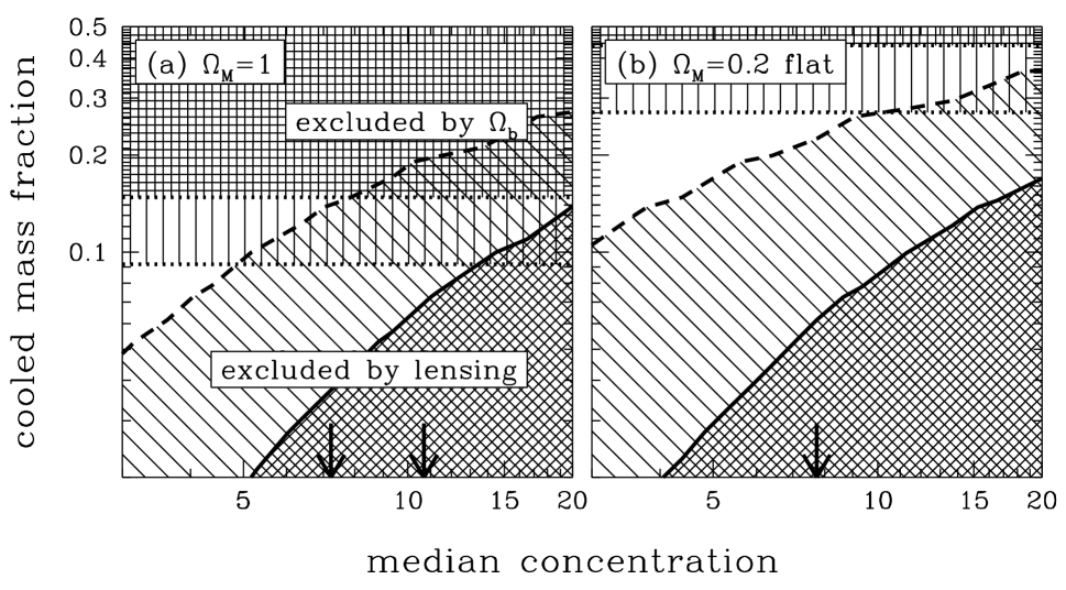
Figure 4: Confidence regions in the $({\hat{C}},f_{cool})$ plane for the fiducial models. The shaded regions below the diagonal curves are excluded at 95% confidence by the lens data; the lower and upper curves correspond to the $N$ and $\theta$ tests, respectively. The shaded regions above the horizontal lines are excluded by measurements of the cosmic baryon density $\Omega_{b}$. The lower curve corresponds to $\Omega_{b}h^{2}=0.019\pm 0.0024$ from measurements of deuterium (Tytler et al. 2000), and the upper curve corresponds to $\Omega_{b}h^{2}<0.037$ (95% confidence) from the cosmic microwave background (Tegmark et al. 2001). The arrows on the $x$-axes indicate concentrations predicted by CDM simulations (see text). Results are shown for two cosmologies.

Comparing the models to the data using the $N$ and $\theta$ statistical tests yields confidence limits on the model parameters, as shown in Figure 4. There is a band in the upper left of the $({\hat{C}},f_{cool})$ plane where the models are consistent with both the number of lenses and the distribution of image separations. Moving to larger ${\hat{C}}$ or smaller $f_{cool}$ increases the number and sizes of predicted lenses. In the hatched region, the predicted lenses are generally too big, and the models are ruled out (at 95% confidence) by the $\theta$ test. In the cross-hatched region, the models are further excluded because they predict too many lenses (the $N$ test). The contours from the $N$ test are based on the assumption that 16 CLASS lenses are produced by elliptical galaxies. If the number of CLASS lenses with elliptical galaxies turns out to be smaller than 16, the $N$ contours would move further up and to the left, strengthening the constraints from lensing.

There is little difference between the lensing constraints in the two cosmologies shown in Figure 4, which seems surprising because it is traditionally argued that lens statistics are quite sensitive to a cosmological constant $\Lambda$ (e.g., Turner 1990; Kochanek 1996). The traditional argument is based on models where the lens galaxy population is obtained by taking the local comoving number density of galaxies and assuming that it holds out to redshift $z\sim 1$ in all cosmologies; in this case, the number of lenses is very sensitive to the volume of the universe to $z\sim 1$, and hence to $\Lambda$. By contrast, my models are based on counts of galaxies at $z\sim 0.5$ from the CNOC2 field galaxy redshift survey (Lin et al. 1999, 2001). In these models, the volume factor required to convert from number counts to number density (or luminosity function) essentially cancels the volume factor that appears in the lensing analysis; the number of lenses is roughly proportional to the number counts of galaxies, and is not very sensitive to $\Lambda$. In other words, using models normalized by number counts of galaxies at $z\sim 0.5$ makes lens statistics only weakly sensitive to cosmology.

CDM simulations make specific predictions about the concentration: in a cosmology with $\Omega_{M}=1$, ${\hat{C}}\simeq 11$ for standard CDM, or ${\hat{C}}\simeq 7$ for tilted CDM where the power spectrum has shape parameter $\Gamma=0.2$; and in an $\Omega_{M}=0.2$ flat cosmology, ${\hat{C}}\simeq 8$ (Navarro et al. 1997). These values are indicated by arrows on the $x$-axes in Figure 4. Cosmic baryon censuses give limits on $f_{cool}$. Because $f_{cool}$ gives the fraction of a system’s mass that has cooled into the baryonic galaxy, it is a lower limit on the baryonic content of the system and hence should not exceed the cosmic baryon fraction, $\Omega_{b}/\Omega_{M}$ (e.g., White et al. 1993). The upper limits on $f_{cool}$ derived from measurements of $\Omega_{b}$ using the cosmic microwave background (e.g., Tegmark, Zaldarriaga & Hamilton 2001) and the deuterium/hydrogen ratio and big bang nucleosynthesis (e.g., Tytler et al. 2000) are indicated by horizontal lines in Figure 4. Some elliptical galaxies contain hot, X-ray emitting gas that is probably primordial gas that never cooled; the cool stellar component may contain as little as half of the baryons (e.g., Brighenti & Mathews 1998). The presence of hot gas would reduce the upper limit on $f_{cool}$ to something below $\Omega_{b}/\Omega_{M}$; but because the actual amount of gas and its presence across the galaxy population are not well understood, I focus on the conservative upper limit from $\Omega_{b}$.

The lens data reject models where concentrated, massive dark matter halos make elliptical galaxies overly efficient lenses — a large portion of the $({\hat{C}},f_{cool})$ plane. At the concentrations found in CDM simulations, lensing requires baryon fractions that are incompatible with a high-density universe. The lens data are formally compatible with a low-density universe, but only in a narrow corner of parameter space where galaxy-mass halos must be very efficient at cooling their baryons. The general conclusion, then, is that galaxies constructed from CDM mass distributions are too concentrated to agree with lens statistics, especially in a high-density CDM cosmology.

There is clearly a degeneracy between ${\hat{C}}$ and $f_{cool}$ in Figure 4, which is not surprising because both parameters affect the central mass that determines the lensing properties. It is therefore interesting to define an integral quantity,

$${\cal M}(r)\equiv\left\langle{M_{halo}(r)\over M_{gal}(r)}\right\rangle,$$ (20)

which is the ratio of halo mass to galaxy mass inside some radius $r$, where the average is over the lens population. Note that ${\cal M}$ is defined using the mass in spheres. The mass ratio allows model-independent statements about the dark matter distribution in early-type galaxies, which are summarized in Table 1. In the fiducial models, dark matter can account for up to 29–33% of the mass inside $R_{e}$ (95% confidence upper limit), and up to 35–40% of the total mass inside $2R_{e}$. In other words, dark matter can contribute a moderate fraction of the mass in the inner regions of elliptical galaxies, but it is not the dominant mass component at small radii. These interesting upper limits result from the distribution of image separations; observed lenses are too small to be consistent with larger dark matter contributions. The lensing limits are similar to but stronger than those derived from a dynamical analysis of the nearby elliptical galaxy NGC 2434 (Rix et al. 1997). They are consistent with the lower limits on dark matter in ellipticals derived from the relationship between X-ray temperature and stellar velocity dispersion (Loewenstein & White 1999).

Table 1
Halo/Galaxy Mass Ratio
	Radius	$\Omega_{M}=1$	$\Omega_{M}=0.2$ flat
Case 1	$R_{e}$	${\cal M}<0.50$	${\cal M}<0.41$
	$2R_{e}$	${\cal M}<0.66$	${\cal M}<0.55$
Case 2	$R_{e}$	${\cal M}<0.43$	${\cal M}<0.27$
	$2R_{e}$	${\cal M}<0.57$	${\cal M}<0.35$
Case 3	$R_{e}$	${\cal M}<0.50$	${\cal M}<0.44$
	$2R_{e}$	${\cal M}<0.68$	${\cal M}<0.60$
Case 4	$R_{e}$	${\cal M}<0.50$	${\cal M}<0.41$
	$2R_{e}$	${\cal M}<0.65$	${\cal M}<0.52$

Note. — 95% confidence upper limits on the halo/galaxy mass ratio, defined in eq. (20), computed at two radii for two cosmologies. The four different cases are defined in the text.

4.3 Systematic effects

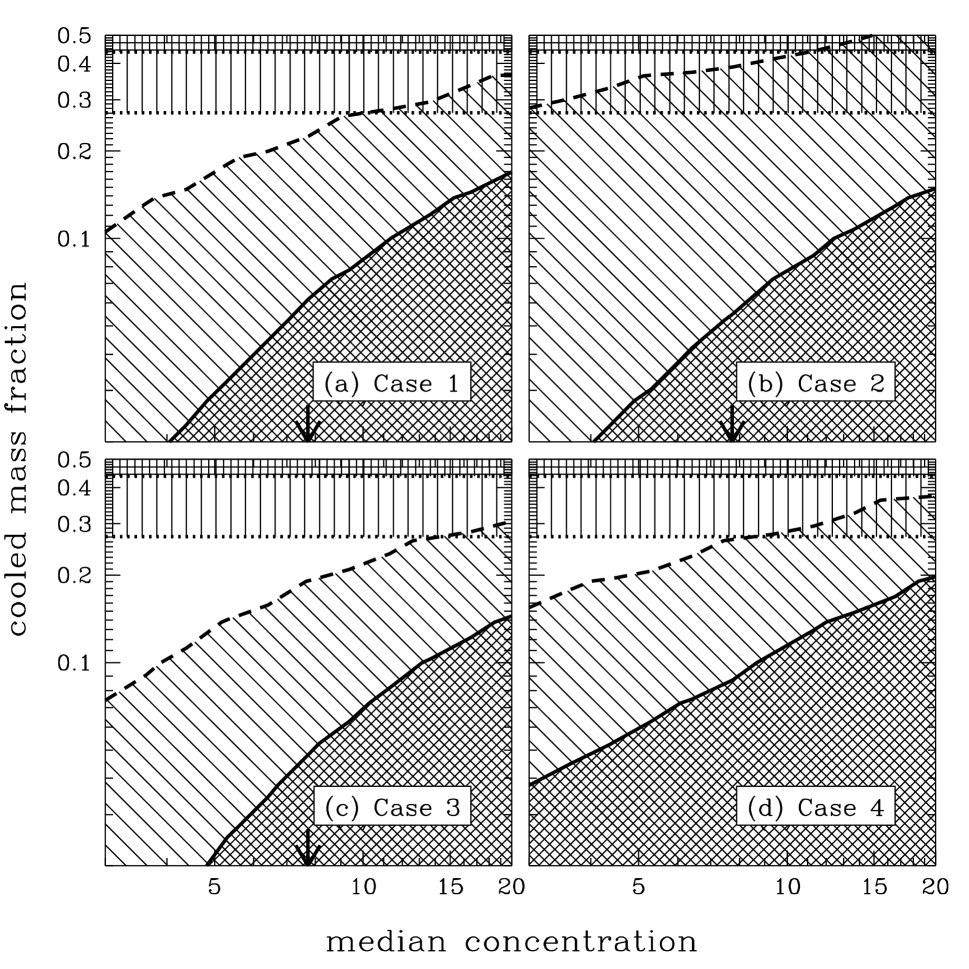
Figure 5: Confidence regions in the $({\hat{C}},f_{cool})$ plane, shown for the four cases defined in the text, in an $\Omega_{M}=0.2$ flat cosmology. Panel (a) is the same as Figure 4b but is included here for completeness.

There are three systematic effects that may be important for the models. Figure 5 shows how the results from the fiducial models (case 1, Figure 5a) are changed by each effect, and Table 1 gives the updated constraints on the halo/galaxy mass ratio ${\cal M}$. In case 2 (Figure 5b), the fixed source redshift is replaced by a redshift distribution to match the CLASS spectroscopic subsample (Marlow et al. 2000). The new models predict larger image separations, so the region excluded by the $\theta$ test stretches up and to the left. While the entire $({\hat{C}},f_{cool})$ plane is now formally excluded either by lensing or by $\Omega_{b}$, it is not clear how strongly to interpret this result, because the CLASS spectroscopic subsample may not fairly represent the full CLASS sample. The strength of the conclusions will ultimately be limited by the extent to which the redshift distribution of the full CLASS sample can be determined. Nevertheless, it is important to discover that the redshift distribution may actually worsen the discrepancy between the data and the models.

In case 3 (Figure 5c), the redshift at which the stellar populations formed is reduced from $z_{f}=5$ to $z_{f}=3$. The younger stellar populations have smaller mass-to-light ratios, so the galaxies are poorer lenses (because the luminosity function is held fixed). Thus, the models predict fewer and smaller lenses, and the regions excluded by lensing move down and to the right in the $({\hat{C}},f_{cool})$ plane. Nevertheless, the changes in the lensing constraints are small; lens statistics are not very sensitive to the galaxy formation redshift, provided that the stellar populations of elliptical galaxies are old. The Fundamental Plane of elliptical galaxies in rich clusters out to $z=0.83$ (e.g., van Dokkum et al. 1998) and of elliptical lens galaxies in low-density environments out to $z\sim 1$ (Kochanek et al. 2000) indeed implies old stellar populations, $z_{f}\gtrsim 2$.

Finally, in case 4 (Figure 5d), the initial NFW profiles are replaced by steeper Moore profiles. Moore halos have more mass in the central regions than NFW halos, even for a fixed concentration parameter, and thus yield better lenses. Hence, the models predict more and larger lenses, and the excluded regions move up and to the left in the $({\hat{C}},f_{cool})$ plane. The change is not very dramatic, however, because of the effects of adiabatic contraction. Moore halos, which are denser than NFW halos to begin with, experience a smaller density enhancement under adiabatic contraction (see Figure 2.1). In other words, adiabatic contraction tends to erase some of the differences between NFW and Moore models.

These results suggest that systematic effects do not weaken the discrepancy between models and data, and may even strengthen it. CDM star+halo models are at best marginally consistent with the statistics of strong lenses, and may be quite inconsistent depending on the distribution of source redshifts in the full CLASS sample. As a relatively model-independent conclusion, the lensed image separations imply that dark matter can contribute no more than about 33% of the total mass inside $R_{e}$, or about 40% of the mass inside $2R_{e}$ (95% confidence; see Table 1). CDM halos appear to be too concentrated to agree comfortably with this constraint.

5 Odd images

In this section, the very inner regions of star+halo models are evaluated with lensing. The fact that most lenses do not show the expected central or “odd” images places strong lower limits on the central densities of galaxies. Section 5.1 reviews the data, Section 5.2 presents results, and Section 5.3 offers a discussion.

5.1 Data

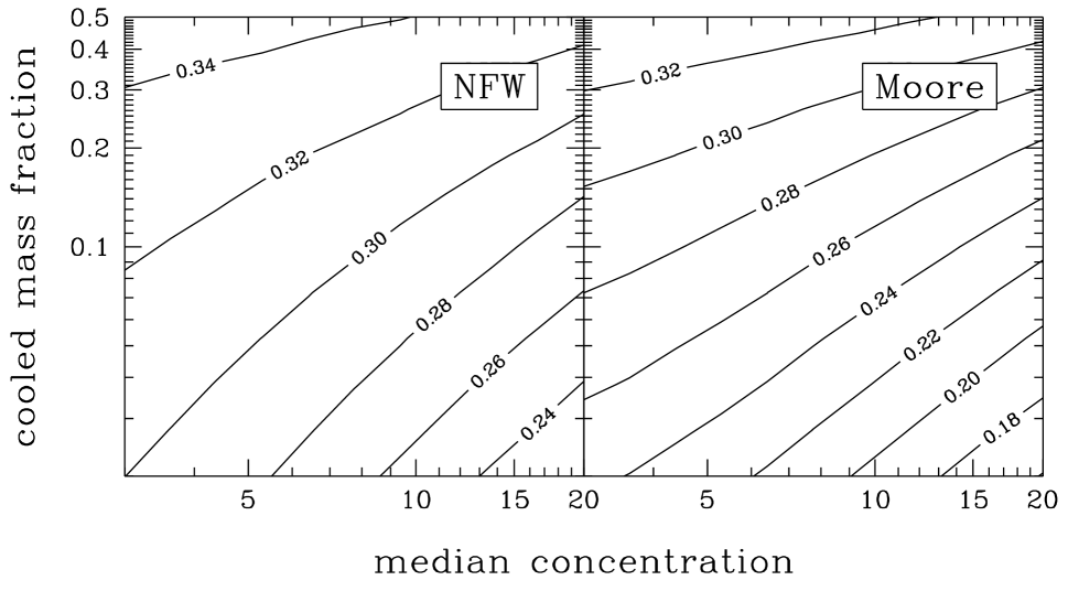
Figure 6: Contours of the fraction of (two-image) lenses where the odd image is brighter than 1% of the brightest image ($f_{odd}\geq 0.01$). Results are shown for an $\Omega_{M}=0.2$ flat cosmology. The left panel shows models with NFW halos (case 1), and the right panel show models with Moore halos (case 4).

It can be proved mathematically that a single thin lens with a smooth (i.e., non-singular) projected mass density and a finite mass always produces an odd number of images (Burke 1981; also see Schneider et al. 1992). In other words, lenses are generally expected to have three or five images, but are usually observed to have two or four. The apparent paradox is resolved by noting that for lenses with high central densities, one of the images is close to the center of the lens and demagnified. If the central density is high enough, the central image may be highly demagnified and therefore very difficult to detect. For example, Appendix B shows that for an isothermal sphere with a small core radius, or for a power law density $\rho\propto r^{-\alpha}$ with $\alpha\approx 2$, the mean magnification of central or “odd” images can be quite small. Every two- or four-image lens may therefore be a three- or five-image system where one of the images remains undetected.

Odd images are expected to be rare in optical observations, because they would be swamped by light from the lens galaxies. The only lens with an odd number of optical images is APM 08279+5255 (Ibata et al. 1999); the third image is either a standard odd image, in which case it requires a shallow density cusp $\alpha\lesssim 0.4$ for $\rho\propto r^{-\alpha}$ (Muñoz et al. 2001), or else it represents a special image configuration produced by an edge-on disk (Keeton & Kochanek 1998). Radio observations should be much more sensitive to odd images, because the lens galaxies (as opposed to the sources) are rarely radio loud. The only candidate odd image detected in the radio is in MG 1131+0456 (Chen & Hewitt 1993), although the possibility that the lens galaxy is radio loud cannot be ruled out in this case.

The CLASS lens sample offers high-resolution and high-dynamic range (noise level $\sim$50 $\mu$Jy beam^-1) radio maps of lenses with compact radio sources, and thus should be quite sensitive to odd images. Consequently, the fact that no CLASS lens shows an odd image leads to strong upper limits on how bright the odd images can be. Rusin & Ma (2001) tabulate the upper limits on six two-image CLASS lenses. To factor out the unknown brightness of the source, they quote upper limits in terms of the flux ratio $f_{odd}$ defined to be the flux of the odd image relative to the flux of the brightest image. The 5$\sigma$ upper limits range from $f_{odd}<0.0083$ for B 0739+366 (Marlow et al. 2001) to $f_{odd}<0.00049$ for B 0218+357 (Biggs et al. 1999). Norbury et al. (2001) give limits on odd images for CLASS lenses with more than two images. When quantifying odd images relative to other lensed images, four-image lenses are much more sensitive to asymmetry in the lens galaxy than two-image lenses. Hence, I restrict attention to the two-image CLASS lenses where spherical models are sufficient for interpreting odd images.

5.2 Results

Figure 7: The cumulative fraction of (two-image) lenses where the ratio of the odd image to the brightest image is greater than $f_{odd}$. Results are shown for models with ${\hat{C}}=7.7$ and $f_{cool}=0.19$, in an $\Omega_{M}=0.2$ flat cosmology. The galaxy components are modeled as $\rho\propto r^{-\alpha}(r_{s}+r)^{\alpha-4}$, and each curve shows results for a particular value of $\alpha$; the fiducial Hernquist model corresponds to $\alpha=1.0$. The initial mass distribution is modeled with an NFW (left panel) or Moore (right panel) profile. The heavy dashed curves show the upper limits derived from six two-image CLASS lenses (Rusin & Ma 2001).

Figure 8: Similar to Figure 7, but showing the effects of supermassive black holes. The dotted curves show results for star+halo models without black holes, for NFW (left panel) and Moore (right panel) models. The solid curves show results when central black holes are added. For the curves labeled “BH,” the black hole masses are normalized by the empirical correlation between black hole mass and galaxy velocity dispersion (Ferrarese & Merritt 2000; Merritt & Ferrarese 2001). In the curves labeled “BH$\times N$,” the black holes are made systematically more massive by the factor $N$. (All galaxies have $\alpha=1.0$.) The heavy dashed curves again show the upper limits from six CLASS.

For power law models with $\rho\propto r^{-1.5}$ the mean magnification of odd images is unity, so odd images are not highly demagnified (see eq. B7 in Appendix B). This simple prediction does not strictly apply to star+halo models, because even in the initial halos the broken power laws affect lensing via projection, and adiabatic contraction increases the central density. However, it does suggest that the odd images in star+halo models are worth investigating. The best way to draw conclusions from observational limits on odd images is to use models of individual systems that take into account not only the detection limits but also constraints on the global lens model from the observed images (e.g., Cohn et al. 2001; Muñoz et al. 2001; Rusin & Ma 2001; Norbury et al. 2001). Instead, in this statistical analysis I examine the distribution of odd images predicted by star+halo models to understand the general trends (c.f., Wallington & Narayan 1993).

The upper limits on odd images in the CLASS doubles range from $f_{odd}<0.0083$ down to $f_{odd}<0.0005$; to be very conservative, we can simply say that no CLASS double has an odd image brighter than $f_{odd}=0.01$. In contrast, Figure 6 shows that star+halo models predict that more than 20% of lenses should have odd images with $f_{odd}\geq 0.01$; and for the range of parameters allowed by the number and sizes of lenses, the fraction is more like 30%. In other words, star+halo models predict that detectable odd images should be quite common, in conflict with observations. This result is not terribly sensitive to the model parameters. It is surprisingly similar for NFW and Moore models, despite the differences in the dark matter cusps. The explanation is again adiabatic contraction: most of the mass in the cores of the galaxies was pulled in by adiabatic contraction, which affects NFW halos more strongly than Moore halos and thus tends to reduce the differences between the two models. The fraction of lenses with detectable odd images is a strong function of the detection threshold (see Figures 7 and 8), so the discrepancy between data and models grows as the upper limit on $f_{odd}$ is decreased.

Odd images are sensitive to the density profile at small radii, so the assumption of a Hernquist model galaxy with a $\rho\propto r^{-1}$ cusp should be examined. Faber et al. (1997), Ravindranath et al. (2001), and Rest et al. (2001) find that the surface brightness distributions $I(R)$ of early-type galaxies have a range of cusps; luminous early-type galaxies have cores or shallow cusps ($I\propto R^{-\gamma}$ with $\gamma\lesssim 0.3$, corresponding to $\rho\propto r^{-\alpha}$ with $\alpha\lesssim 1.3$), while fainter galaxies have steeper power-law cusps. Hence, the Hernquist model seems reasonable for the massive galaxies that dominate lensing. Still, for completeness I consider models where the Hernquist galaxy is generalized to an arbitrary cusp using the density profile $\rho\propto r^{-\alpha}(r_{s}+r)^{\alpha-4}$. Figure 7 shows the results for models with ${\hat{C}}=7.7$ and $f_{cool}=0.19$ (a point close to the $\theta$ boundary in Figure 4). Steep cusps suppress odd images, but only if they are considerably steeper than the luminosity cusps in luminous early-type galaxies. As a corollary, steep cusps also make galaxies more efficient lenses and thus aggravate the discrepancy between the models and the observed number and sizes of lenses. In other words, cusps do not provide a very attractive resolution to the odd image problem. These conclusions apply to both NFW and Moore dark matter models.

The simple star+halo models may not be sufficient for this analysis, because many galaxies are observed to contain central supermassive black holes (e.g., Magorrian et al. 1998; Gebhardt et al. 2000a, 2000b; Ferrarese & Merritt 2000; Merritt & Ferrarese 2001). While black holes have little effect on the number and sizes of lenses (they barely affect the potential on kiloparsec scales), they may suppress or even eliminate odd images (Mao, Witt & Koopmans 2001). To understand their effects on lens statistics, I add black holes to the star+halo models, where the mass of the black hole is determined from the velocity dispersion of the galaxy using the empirical correlation $M_{bh}=(1.30\pm 0.36)\times 10^{8}\,M_{\odot}\,(\sigma/200\,\mbox{km s${}^{-1}$})^{4.72\pm 0.36}$ (Ferrarese & Merritt 2000; Merritt & Ferrarese 2001). Figure 8 shows that black holes normalized by this relation have little effect on odd images down to $f_{odd}\sim 0.001$. Making the black holes systematically more massive increases the suppression, but only for the faintest odd images. Black holes must lie off the Ferrarese & Merritt relation by at least a factor of 10 in mass before they begin to affect odd images at the $f_{odd}=0.01$ level. These conclusions again apply with almost equal strength to NFW and Moore models.

5.3 Discussion

When compared to the current limits from CLASS, the star+halo models clearly predict too many detectable odd images. The discrepancy is not easily resolved by changing the density profile or invoking supermassive black holes. In other words, galaxies constructed from CDM mass distributions have central densities that are too low. This conclusion is consistent with the result from Rusin & Ma (2001) that the lack of odd images requires steep density profiles, $\rho\propto r^{-\alpha}$ with $\alpha>1.8$ at 90% confidence. Given that the measurements of odd images are only upper limits, the constraints from odd images can only get stronger — and perhaps substantially, if more lenses turn out to have upper limits as strong as $f_{odd}<0.0005$ in B 0218+357.

The odd image problem stands in stark contrast to most observational tests of CDM. Spiral galaxy dynamics are said to imply that CDM halos are too concentrated to agree with observed galaxies (e.g., Moore 1994; de Blok et al. 2001; Salucci 2001; Weiner et al. 2001), although there is still substantial debate about whether beam smearing affects this conclusion for low surface brightness galaxies (van den Bosch et al. 2000; van den Bosch & Swaters 2000). Independent of the dynamical arguments, the number and sizes of observed lenses lead to a similar conclusion, as shown in §4. Recent interest in modifications to CDM, such as self-interacting dark matter (e.g., Spergel & Steinhardt 2000; see Wandelt et al. 2000 for a review), has therefore focused on making dark matter halos less concentrated. However, the lack of odd images implies that galaxies built from CDM halos are not concentrated enough, to a significant degree. If self-interacting dark matter reduces densities, it would only exacerbate the odd image problem.

It is clearly important to understand and resolve this paradox. Perhaps it is a case of comparing different samples. Lensing intrinsically selects dense, massive galaxies, so most lenses are elliptical galaxies; by contrast, the dynamical arguments against CDM halos come primarily from spiral galaxies, and in particular low surface brightness galaxies. However, the strongest limit on an odd image actually comes from a lens produced by a face-on spiral galaxy ($f_{odd}<0.0005$ for B 0218+357).

More likely, it is a question of scales. Dynamical observations and observed lensed images probe scales from several kiloparsecs down to $\sim$0.5 kpc, while odd images probe scales more like tens of parsecs. The paradox could be resolved if halos have high densities on $\sim$10 pc scales, low mean densities at $\sim$1 kpc, and substantial dark matter halos beyond several kiloparsecs. The star+halo models do not show the required small-scale structure — but they are based on a questionable extrapolation of CDM profiles to scales much smaller than the resolution of numerical simulations. On such small scales, other effects may be important; while supermassive black holes appear not to suppress odd images at the required levels, self-interacting dark matter may be a mechanism to steepen the central cusp (Burkert 2000; Kochanek & White 2000; Moore et al. 2000), or simply to concentrate a lot of dark matter at very small radii (Ostriker 2000). Regardless of what the correct explanation turns out to be, it is clear that the odd image problem provides a very interesting probe of galaxy mass distributions in the inner tens of parsecs.

6 Conclusions

Star+halo models of elliptical galaxies are a natural outgrowth of the Cold Dark Matter paradigm that can reproduce the quasi-isothermal mass distributions implied by stellar dynamics, X-ray halos, and gravitational lensing. When the stellar components are fixed by observed galaxy populations, gravitational lens statistics can be used to constrain the dark matter components. The observed number and sizes of lenses place important upper limits on the amount of dark matter in the inner regions of elliptical galaxies: on average, dark matter can account for no more than about 33% of the total mass inside one effective radius ($R_{e}$), or about 40% of the mass inside $2R_{e}$ (95% confidence upper limits). Lensed images typically appear at a few effective radii, so the stellar and dark matter components must be comparably important for lensing.

The dark matter limits are interesting when interpreted in the context of the CDM paradigm. Galaxies built from CDM mass distributions have significant amounts of central dark matter, so they predict that lenses should be more numerous and larger than observed. A high-density ($\Omega_{M}=1$) CDM cosmology can therefore be ruled out at better than 95% confidence, while a low-density, flat cosmology ($\Omega_{M}=0.2$, $\Omega_{\Lambda}=0.8$) is at best marginally consistent with the lens data. By implying that CDM model galaxies have too much mass on kiloparsec scales, lensing independently supports the evidence against CDM from spiral galaxy dynamics (e.g., Moore 1994; de Blok et al. 2001; Salucci 2001; Weiner et al. 2001). The evidence from lensing is important because its only uncertainty is the decomposition into stellar and dark matter components, and lensing extends the argument to elliptical galaxies. These conclusions may be invalid if simple adiabatic contraction models do not apply to elliptical galaxies, but the models appear to agree well with simulated galaxies even in merger scenarios (Gottbrath 2000).

Lensing offers a unique additional insight into galaxy mass distributions. Star+halo models predict that a central or “odd” image should be detectable in more than 30% of lenses, but such images are rarely observed. Equivalently, the upper limits on the fluxes of odd images for CLASS lenses lead to strong lower limits on the central densities of lens galaxies, and star+halo models fail to satisfy the limits. The failure is perhaps not surprising, because odd images are sensitive to the mass distribution on scales of tens of parsecs, where simple CDM models may break down. For example, supermassive black holes, which appear to be common in the centers of galaxies (e.g., Magorrian et al. 1998; Gebhardt et al. 2000a, 2000b; Ferrarese & Merritt 2000; Merritt & Ferrarese 2001), might reconcile the models with the data by helping to suppress odd images (see Mao et al. 2001). However, star+halo models would need black holes that lie off the observed black hole–bulge mass correlation by more than a factor of 10 in order to suppress odd images at the required level. Alternatively, steeper central cusps could suppress odd images, but only if mass cusps are considerable steeper than luminosity cusps, only if steep cusps can survive merger events (which is unlikely if the progenitors contain black holes; Milosavljević & Merritt 2001), and only at the expense of aggravating the discrepancy in the number and sizes of lenses.

The evidence from the number and sizes of lenses (and from spiral galaxy dynamics) implies, then, that CDM mass distributions have too much mass on kiloparsec scales; and the odd image problem indicates too little mass on tens of parsec scales. The problem may be the assumption that the dark matter particles are collisionless. Allowing dark matter self-interactions can lower the density on large scales (e.g., Spergel & Steinhardt 2000; Burkert 2000; Davé et al. 2001), although matching observations may require substantial fine tuning (e.g., Kochanek & White 2000; Moore et al. 2000; Yoshida et al. 2000). As an intriguing corollary, Ostriker (2000) proposes that self-interactions could also increase the dark matter density on very small scales. Self-interacting dark matter models might therefore provide a way to reconcile cosmological mass models with real galaxies over a wide range of spatial scales, although the details remain to be worked out. In any case, it appears that lensing will be a very important test of modifications to CDM through its ability to simultaneously test mass distributions on large scales (via observed images) and small scales (via limits on, and eventually detections of, odd images). These tests based on galaxy-scale lenses will complement constraints on self-interacting dark matter from giant arcs produced by cluster lenses (Meneghetti et al. 2001).

It would be interesting to apply star+halo models to individual lenses, especially given the statistical limits implying that the stellar and dark matter components are of comparable importance in lensing. Comparing the halo/galaxy mass ratios inferred for individual lenses with the limits from statistics would be an important test of the models. Using two independent components would make it possible to to examine whether the stellar and halo distributions have similar or different ellipticities and orientations, although the decomposition may not be unique. Finally, using two components with different ellipticities and/or orientations would test whether single-component lens models are sufficient or oversimplified. In particular, star+halo models might provide an internal reason why most lenses cannot be fit by a single ellipsoidal mass distribution (e.g., Keeton, Kochanek & Seljak 1997), although internal effects may often be smaller than external tidal perturbations from objects near the lens galaxy or along the line of sight (e.g., Hogg & Blandford 1994; Schechter et al. 1997).

The constraints on dark matter from lens statistics can be strengthened with better data in at least three ways. First, the strongest constraints come from the distribution of image separations, where the model predictions are sensitive to the redshift distribution of the CLASS sample. The CLASS spectroscopic subsample (Marlow et al. 2000) provides a useful starting point, but the redshift distribution of the full sample must be better constrained to make the lensing analysis truly robust. Second, many of the current constraints on odd images lie at the $f_{odd}\simeq 0.01$ level (Rusin & Ma 2001). If the limits could be improved to the $f_{odd}\simeq 0.003$ level or better, they would make the models much more sensitive to supermassive black holes, and lensing would become a powerful probe of black holes in distant galaxies out to redshift $z\sim 1$. Finally, this analysis is based primarily on the sample of lenses from the CLASS survey, which is the largest existing lens survey but still has only 18 lenses. Larger surveys, in particular the Sloan Digital Sky Survey (SDSS; York et al. 2000), should increase the number of lenses by well over an order of magnitude. The SDSS lens sample will dramatically improve the constraints from lensing, provided that selection effects are well understood and that there is a subsample of radio loud lenses where useful limits on odd images can be obtained.

Appendix A An Analytic Solution of Adiabatic Contraction

Blumenthal et al. (1986) give a simple analytic treatment of spherical adiabatic contraction that agrees remarkably well with more detailed numerical simulations. Let $M_{i}(r_{i})$ be the initial mass profile as a function of the initial radius $r_{i}$, while $M_{g}(r)$ and $M_{h}(r)$ are the final mass profiles of the galaxy and halo, respectively. In the Blumenthal et al. (1986) prescription, the three profiles are related by two equations,

$$r\,\left[M_{g}(r)+M_{h}(r)\right]=r_{i}\,M_{i}(r_{i})\,,$$ (A1)

$$M_{h}(r)=(1-f_{cool})M_{i}(r_{i})\,,$$ (A2)

where $f_{cool}=M_{g,tot}/M_{i,tot}$ is the fraction of the system’s mass contained in baryons that cool to form the galaxy. (There can be other baryons that remain hot and distributed throughout the halo, but they do not affect adiabatic contraction.)

This adiabatic contraction formalism has often been applied to the problem of a disk galaxy in an NFW halo. Rix et al. (1997) have computed adiabatic contraction for elliptical galaxies numerically, but I find that with a Hernquist model (eq. 1 in §2.1) the problem can be solved analytically. Each initial radius $r_{i}$ maps to a unique final radius $r$ given by the solution of the equation

$$f_{cool}\,r^{3}+(r+s_{g})^{2}\left[(1-f_{cool})r-r_{i}\right]m_{i}(r_{i})=0\,,$$ (A3)

which is a cubic polynomial in $r$. Note that I have take the galaxy scale radius $r_{s}$ from eq. (1) and relabeled it as $s_{g}$. Also, $m_{i}(r_{i})=M_{i}(r_{i})/M_{200}$ is the initial mass profile normalized by the virial mass (the mass inside the virial radius $r_{200}$). In the limit $r\gg s_{g}$, eq. (A3) has the simple asymptotic solution

$$r={r_{i}\,m_{i}(r_{i})\over f_{cool}+(1-f_{cool})m_{i}(r_{i})}\ .$$ (A4)

The full general solution can be also be found analytically, although it cannot be written quite so compactly. Following Abramowitz & Stegun (1981), solve a cubic equation of the form

$$z^{3}+a_{2}z^{2}+a_{1}z+a_{0}=0$$ (A5)

by defining

$$p = {a_{1}a_{2}-3a_{0}\over 6}-{a_{2}^{3}\over 27}\,,$$ (A6)

$$q = {a_{1}\over 3}-{a_{2}^{2}\over 9}\,,$$ (A7)

$$s_{1} = \left(p+\sqrt{q^{3}+p^{2}}\right)^{1/3},$$ (A8)

$$s_{2} = \left(p-\sqrt{q^{3}+p^{2}}\right)^{1/3}.$$ (A9)

There is always a real solution of eq. (A5) at

$$z_{1}=(s_{1}+s_{2})-{a_{2}\over 3}\ .$$ (A10)

There are two other roots that may be real or complex, but because the $r_{i}\to r$ mapping under adiabatic contraction should be one-to-one, only the single real root is relevant. Once the cubic equation has been solved to map $r_{i}$ to $r$, eq. (A1) can be used to write the total mass profile as

$$M_{tot}(r)\equiv M_{g}(r)+M_{h}(r)={r_{i}\over r}\,M_{i}(r_{i})\,.$$ (A11)

This solution of adiabatic contraction by a Hernquist galaxy can be used for any form of the initial halo, by simply inserting the desired initial profile $M_{i}(r_{i})$ into eqs. (A3) and (A11).

Appendix B The Mean Magnification of Odd Images

The mean magnification of odd images can be computed analytically, at least for simple lens models. Neglecting magnification bias, the mean magnification is defined to be

$$\langle{\mu_{odd}}\rangle={{\int\mu_{odd}({\bf u})\,d{\bf u}}\over{\int d{\bf u}}}\ ,$$ (B1)

where the integrals extend over the multiply-imaged region of the source plane. Changing variables in the numerator to integrate in the image plane yields

$$\langle{\mu_{odd}}\rangle={{\int_{odd}d{\bf x}}\over{\int d{\bf u}}}\ ,$$ (B2)

where the integral in the numerator extends over the region in the image plane where odd images are found. The result is so simple because the $\mu_{odd}({\bf u})$ factor in eq. (B1) is exactly cancelled by the Jacobian of the coordinate transformation. Eq. (B2) says that the mean odd image magnification is simply the area where odd images occur in the image plane divided by the area of the multiply-imaged region of the source plane. This result is general and does not require specific symmetries in the lens model. It can be generalized to other types of images as well, provided that multiplicities are properly counted.

Now focusing on spherical systems, $\langle{\mu_{odd}}\rangle=(r_{cr}/u_{out})^{2}$ where $r_{cr}$ is the radial critical curve and $u_{out}$ is the boundary of the multiply-imaged region (see §3). These radii are found as follows. The critical radius is the solution of the equation

$${d\phi_{R}\over dR}\biggr{|}_{R=r_{cr}}=1,$$ (B3)

where $\phi_{R}$ is the lensing deflection. The boundary of the multiply-imaged region is then

$$u_{out}=(\phi_{R}-R)\bigr{|}_{R=r_{cr}}.$$ (B4)

Consider two simple models. First, for a softened isothermal sphere with density $\rho\propto(s^{2}+r^{2})^{-1}$ with core radius $s$,

$$\langle{\mu_{odd}}\rangle = {{4s}\over(\sqrt{4r_{E}+s}-3\sqrt{s})^{2}}\ ,$$ (B5)

$$= {s\over r_{E}}+3\left({s\over r_{E}}\right)^{3/2}+{13\over 2}\,\left({s\over r_{E}}\right)^{2}+{\cal O}\left({s\over r_{E}}\right)^{5/2},$$ (B6)

where $r_{E}$ is the Einstein ring radius of the model when the core radius is zero. Second, for a simple power law density $\rho\propto r^{-\alpha}$ (with $\alpha>1$ to ensure that the projected mass distribution is a decreasing function of radius),

$$\langle{\mu_{odd}}\rangle=\cases{[(2-\alpha)/(\alpha-1)]^{2}&if $1<\alpha<2$\cr 0&if $\alpha\geq 2$\cr}$$ (B7)

Note that for $\alpha\geq 2$ the model does not produce odd images (the density is singular, so the odd image theorem does not apply; see §5.1), so $\langle{\mu_{odd}}\rangle\equiv 0$.

References

- (1)
- (2) Abramowitz, M., & Stegun, I. A. 1981, Handbook of mathematical functions with formulas, graphs, and mathematical tables (Washington: National Bureau of Standards)
- (3)
- (4) Barkana, R. 1998, ApJ, 502, 531
- (5)
- (6) Bartelmann, M. 1996, A&A, 313, 697
- (7)
- (8) Biggs, A. D., Browne, I. W. A., Helbig, P., Koopmans, L. V. E., Wilkinson, P. N., & Perley, R. A. 1999, MNRAS, 304, 349
- (9)
- (10) Binggeli, B., & Cameron, L. A. 1991, A&A, 252, 27
- (11)
- (12) Binggeli, B., & Cameron, L. A. 1993, A&AS, 98, 297
- (13)
- (14) Blais-Ouellette, S., Amram, P., & Carignan, C. 2001, AJ, 121, 1952
- (15)
- (16) Blumenthal, G., Faber, S., Flores, R., & Primack, J. 1986, ApJ, 301, 27
- (17)
- (18) Brighenti, F., & Mathews, W. G. 1998, ApJ, 495, 239
- (19)
- (20) Browne, I. W. A. 2001, in Gravitational Lensing: Recent Progress and Future Goals (ASP), ed. T. Brainerd & C. S. Kochanek
- (21)
- (22) Bruzual, G., & Charlot, S. 1993, ApJ, 405, 538
- (23)
- (24) Bullock, J. S., Kolatt, T. S., Sigad, T., Somerville, R. S., Kravtsov, A. V., Klypin, A. A., Primack, J. R., & Dekel, A. 2001, MNRAS, 321, 559
- (25)
- (26) Burke, W. L. 1981, ApJ, 244, L1
- (27)
- (28) Burkert, A. 2000, ApJ, 534, L143
- (29)
- (30) Carroll, S. M., Press, W. H., & Turner, E. L. 1992, ARA&A, 30, 499
- (31)
- (32) Chae, K.-H., Khersonsky, V. K., & Turnshek, D. A. 1998, ApJ, 506, 80
- (33)
- (34) Chen, G. H., & Hewitt, J. N. 1993, AJ, 106, 1719
- (35)
- (36) Cohn, J. D., Kochanek, C. S., McLeod, B. A., & Keeton, C. R. 2001, ApJ, in press (also preprint astro-ph/0008390)
- (37)
- (38) Cole, S., & Lacey, C. 1996, MNRAS, 281, 716
- (39)
- (40) Crone, M. M., Evrard, A. E., & Richstone, D. O. 1994, ApJ, 434, 402
- (41)
- (42) Davé, R., Spergel, D. N., Steinhardt, P. J., & Wandelt, B. D. 2001, ApJ, 547, 574
- (43)
- (44) Debattista, V. P., & Sellwood, J. A. 1998, ApJ, 493, L5
- (45)
- (46) de Blok, W. J. G., McGaugh, S. S., Bosma, A., & Rubin, V. C. 2001, ApJ, 552, L23
- (47)
- (48) Djorgovski, S., & Davis, M. 1987, ApJ, 313, 59
- (49)
- (50) Dressler, A., Lynden-Bell, D., Burstein, D., Davies, R. L., Faber, S. M., Terlevich, R., & Wegner, G. 1987, ApJ, 313, 42
- (51)
- (52) Drinkwater, M. J., Webster, R. L., Francis, P. J., Condon, J. J., Ellison, S. L., Jauncey, D. L., Lovell, J., Peterson, B. A., & Savage, A. 1997, MNRAS, 284, 85
- (53)
- (54) Dubinski, J. 1994, ApJ, 431, 617
- (55)
- (56) Eke, V., Navarro, J. F., & Steinmetz, M. 2000, preprint (astro-ph/0012337)
- (57)
- (58) Fabbiano, G. 1989, ARA&A, 27, 87
- (59)
- (60) Falco, E. E., Kochanek, C. S., & Muñoz, J. A. 1998, ApJ, 494 47
- (61)
- (62) Ferrarese, L., & Merritt, D. 2000, ApJ, 539, L9
- (63)
- (64) Flores, R. A., Primack, J. R., Blumenthal, G. R., & Faber, S. M. 1993, ApJ, 412, 443
- (65)
- (66) Flores, R. A., & Primack, J. R. 1994, ApJ, 427, L1
- (67)
- (68) Gebhardt, K., et al. 2000a, ApJ, 539, L13
- (69)
- (70) Gebhardt, K., et al. 2000a, ApJ, 543, L5
- (71)
- (72) Gottbrath, C. 2000, MS thesis, University of Arizona
- (73)
- (74) Haehnelt, M. G., & Kauffmann, G. 2000, MNRAS, 318, L35
- (75)
- (76) Helbig, P. 2000, preprint (astro-ph/0008197)
- (77)
- (78) Henstock, D. R., Browne, I. W. A., Wilkinson, P. N., & McMahon, R. G. 1997, MNRAS, 290, 380
- (79)
- (80) Hernquist, L. 1990, ApJ, 356, 359
- (81)
- (82) Hogg, D. W., & Blandford, R. D. 1994, MNRAS, 268, 889
- (83)
- (84) Huss, A., Jain, B., & Steinmetz, M. 1999a, ApJ, 517, 64
- (85)
- (86) Huss, A., Jain, B., & Steinmetz, M. 1999b, MNRAS, 308, 1011
- (87)
- (88) Ibata, R. A., Lewis, G. F., Irwin, M. J., Lehár, J., & Totten, E. J. 1999, AJ, 118, 1922
- (89)
- (90) Jing, Y. P., & Suto, Y. 2000, ApJ, 529, L69
- (91)
- (92) Keeton, C. R., Kochanek, C. S., & Seljak, U. 1997, ApJ, 482, 604
- (93)
- (94) Keeton, C. R. 1998, PhD thesis, Harvard University
- (95)
- (96) Keeton, C. R., & Kochanek, C. S. 1998, ApJ, 495, 157
- (97)
- (98) Keeton, C. R., & Madau, P. 2001, ApJ, 549, L25
- (99)
- (100) Keeton, C. R. 2001, preprint (astro-ph/0102341)
- (101)
- (102) Klypin, A., Kravtsov, A. V., Bullock, J. S., & Primack, J. R. 2000, preprint (astro-ph/0006343)
- (103)
- (104) Kochanek, C. S. 1993, ApJ, 419, 12
- (105)
- (106) Kochanek, C. S. 1995, ApJ, 445, 559
- (107)
- (108) Kochanek, C. S. 1996, ApJ, 466, 638
- (109)
- (110) Kochanek, C. S., Falco, E. E., Impey, C. D., Lehár, J., McLeod, B. A., Rix, H.-W., Keeton, C. R., Muñoz, J. A., & Peng, C. Y. 2000, ApJ, 543, 131
- (111)
- (112) Kochanek, C. S., Falco, E. E., Impey, C. D., Lehár, J., McLeod, B. A., & Rix, H.-W. 2001, CfA/Arizona Space Telescope Lens Survey web site (http://cfa-www.harvard.edu/castles)
- (113)
- (114) Kochanek, C. S., & White, M. 2000, ApJ, 543, 514
- (115)
- (116) Kochanek, C. S., & White, M. 2001, preprint (astro-ph/0102334)
- (117)
- (118) Lin, H., Yee, H. K. C., Carlberg, R. G., Morris, S. L., Sawicki, M., Patton, D. R., Wirth, G., & Shepherd, C. W. 1999, ApJ, 518, 533
- (119)
- (120) Lin, H., et al. 2001, in preparation
- (121)
- (122) Loewenstein, M., & White, R. E. 1999, ApJ, 518, 50
- (123)
- (124) Magorrian, J., et al. 1998, AJ, 115, 2285
- (125)
- (126) Marlow, D. R., Rusin, D., Jackson, N., Wilkinson, P. N., Browne, I. W. A., & Koopmans, L. 2000, AJ, 119, 2629
- (127)
- (128) Marlow, D. R., et al. 2001, AJ, 121, 619
- (129)
- (130) Mao, S., Witt, H. J., & Koopmans, L. V. E. 2001, MNRAS, 323, 301
- (131)
- (132) Maoz, D., & Rix, H.-W. 1993, ApJ, 416, 425
- (133)
- (134) McGaugh, S. S., & de Blok, W. J. G. 1998, ApJ, 499, 41
- (135)
- (136) Meneghetti, M., Yoshida, N., Bartelmann, M., Moscardini, L., Springel, V., Tormen, G., & White, S. D. M. 2001, MNRAS, 325, 435
- (137)
- (138) Merritt, D., & Ferrarese, L. 2001, ApJ, 547, 140
- (139)
- (140) Milosavljević, M., & Merritt, D. 2001, preprint (astro-ph/0103350)
- (141)
- (142) Moore, B. 1994, Nature, 370, 629
- (143)
- (144) Moore, B., Governato, F., Quinn, T., Stadel, J., & Lake, G. 1998, ApJ, 499, L5
- (145)
- (146) Moore, B., Quinn, T., Governato, F., Stadel, J., & Lake, G. 1999, MNRAS, 310, 1147
- (147)
- (148) Moore, B., Gelato, S., Jenkins, A., Pearce, F. R., & Quilis, V. 2000, ApJ, 535, L21
- (149)
- (150) Moore, B. 2001, preprint (astro-ph/0103100)
- (151)
- (152) Muñoz, J. A., Kochanek, C. S., & Keeton, C. R. 2001, ApJ, in press (also preprint astro-ph/0103009)
- (153)
- (154) Navarro, J. F., Frenk, C. S., & White, S. D. M. 1996, ApJ, 462, 563
- (155)
- (156) Navarro, J. F., Frenk, C. S., & White, S. D. M. 1997, ApJ, 490, 493
- (157)
- (158) Navarro, J. F., & Steinmetz, M. 2000, ApJ, 528, 607
- (159)
- (160) Norbury, M., et al. 2001, MNRAS, submitted
- (161)
- (162) Ostriker, J. P. 2000, Phys. Rev. Lett., 84, 5258
- (163)
- (164) Phillips, P., et al. 2001, MNRAS, submitted
- (165)
- (166) Porciani, C., & Madau, P. 2000, ApJ, 532, 679
- (167)
- (168) Press, W. H., Teukolsky, S. A., Vetterling, W. T., & Flannery, B. P. 1992, Numerical Recipes in C: The Art of Scientific Computing, Second Edition (New York: Cambridge Univ. Press)
- (169)
- (170) Ravindranath, S., Hi, L. C., Peng, C. Y., Filippenki, A. V., & Sargent, W. L. W. 2001, preprint (astro-ph/0105390)
- (171)
- (172) Rest, A., van den Bosch, F. C., Jaffe, W., Tran, H., Tsvetanov, Z., Ford, H. C., Davies, J., & Schafer, J. 2001, AJ, 121, 2431
- (173)
- (174) Rix, H.-W., de Zeeuw, P. T., Cretton, N., van der Marel, R. P., & Carollo, C. M. 1997, ApJ, 488, 702
- (175)
- (176) Rusin, D., & Ma, C.-P. 2001, ApJ, 549, L33
- (177)
- (178) Rusin, D., & Tegmark, M. 2001, ApJ, 553, 709
- (179)
- (180) Salucci, P., & Burkert, A. 2000, ApJ, 537, L9
- (181)
- (182) Salucci, P. 2001, MNRAS, 320, L1
- (183)
- (184) Schade, D., Barrientos, L. F., & López-Cruz, O. 1997, ApJ, 477, L17
- (185)
- (186) Schechter, P. L. 1976, ApJ, 203, 297
- (187)
- (188) Schechter, P. L., et al. 1997, ApJ, 475, L85
- (189)
- (190) Schneider, P., Ehlers, J., & Falco, E. E. 1992, Gravitational Lenses (New York: Springer)
- (191)
- (192) Spergel, D. N., & Steinhardt, P. J. 2000, Phys. Rev. Lett., 84, 3760
- (193)
- (194) Swaters, R. A., Madore, B. F., & Trewhella, M. 2000, ApJ, 531, L107
- (195)
- (196) Tegmark, M., Zaldarriaga, M., & Hamilton, A. J. S. 2001, Phys. Rev. D, 63, 43007
- (197)
- (198) Turner, E. L. 1980, ApJ, 242, L135
- (199)
- (200) Turner, E. L., Ostriker, J. P., & Gott, J. R. 1984, ApJ, 284, 1
- (201)
- (202) Turner, E. L. 1990, ApJ, 365, L43
- (203)
- (204) Tytler, D., O’Meara, J. M., Suzuki, N., & Lubin, D. 2000, Phys. Scr, 85, 12
- (205)
- (206) van den Bosch, F. C., Robertson, B. E., Dalcanton, J. J., & de Blok, W. J. G. 2000, AJ, 119, 1579
- (207)
- (208) van den Bosch, F. C., & Swaters, R. A. 2000, preprint (astro-ph/0006048)
- (209)
- (210) van Dokkum, P. G., Franx, M., Kelson, D. D., & Illingworth, G. D. 1998, ApJ, 504, L17
- (211)
- (212) Wallington, S., & Narayan, R. 1993, ApJ, 403, 517
- (213)
- (214) Wandelt, B. D., Davé, R., Farrar, G. R., McGuire, P. C., Spergel, D. N., & Steinhardt, P. J. 2000, in Proceedings of Dark Matter 2000 (also preprint astro-ph/0006344)
- (215)
- (216) Weiner, B. J., Sellwood, J. A., & Williams, T. B. 2001, ApJ, 546, 931
- (217)
- (218) White, S. D. M., Navarro, J. F., Evrard, A. E., & Frenk, C. S. 1993, Nature, 366, 429
- (219)
- (220) Wyithe, J. S. B., Turner, E. L., & Spergel, D. N. 2000, preprint (astro-ph/0007354)
- (221)
- (222) York, D. G., et al. 2000, AJ, 120, 1579
- (223)
- (224) Yoshida, N., Springel, V., White, S. D. M., & Tormen, G. 2000, ApJ, 544, L87
- (225)