DASI First Results: A Measurement of the Cosmic Microwave Background Angular Power Spectrum

Abstract

We present measurements of anisotropy in the Cosmic Microwave Background (CMB) from the first season of observations with the Degree Angular Scale Interferometer (DASI). The instrument was deployed at the South Pole in the austral summer 1999–2000, and made observations throughout the following austral winter. We present a measurement of the CMB angular power spectrum in the range $100<l<900$ in nine bands with fractional uncertainties in the range 10–20% and dominated by sample variance. In this paper we review the formalism used in the analysis, in particular the use of constraint matrices to project out contaminants such as ground and point source signals and to test for correlations with diffuse foreground templates. We find no evidence of foregrounds other than point sources in the data, and find a maximum likelihood temperature spectral index $\beta=-0.1\pm 0.2$ (1 $\sigma$), consistent with CMB. We detect a first peak in the power spectrum at $l\sim 200$, in agreement with previous experiments. In addition, we detect a peak in the power spectrum at $l\sim 550$ and power of similar magnitude at $l\sim 800$ which are consistent with the second and third harmonic peaks predicted by adiabatic inflationary cosmological models.

1 Introduction

Subtle temperature fluctuations in the Cosmic Microwave Background (CMB) radiation, first observed by the COBE DMR experiment (Smoot et al. 1992), offer a glimpse of the early Universe at the epoch of matter-radiation decoupling, well before the non-linear gravitational collapse of matter led to the structure we see in the Universe today. The theory of inflation, originally proposed as an explanation for apparent isotropy in the CMB and a spatial curvature near unity (Guth 1981; Linde 1982; Albrecht & Steinhardt 1982), was further developed to predict nearly scale-invariant adiabatic density perturbations arising from quantum fluctuations as the source of inhomogeneity in the Universe (Guth & Pi 1982; Hawking 1982; Starobinsky 1982; Bardeen, Steinhardt, & Turner 1983). On angular scales causally disconnected at the epoch of decoupling ($\gtrsim 1\arcdeg$), anisotropy in the CMB reflects the primordial inhomogeneity of matter (see, e.g., White, Scott, & Silk 1994). On scales smaller than the sound horizon at the time of decoupling, the primordial adiabatic density perturbations force gravity-driven acoustic oscillations in the photon-baryon fluid which lead to a harmonic series of peaks in the CMB angular power spectrum (Bond & Efstathiou 1984; Vittorio & Silk 1984). A detection of a series of peaks in the CMB angular power spectrum would provide strong evidence for the inflationary view of the early Universe, and would make alternate theories of structure formation such as defect models difficult to support (Albrecht et al. 1996). A third harmonic peak of comparable or greater magnitude than the second is the signature of baryonic matter re-compressing in dark matter potential wells — a detection of significant power in the third peak region would strongly support the presence of dark matter in the Universe (Hu & White 1996). Within the context of standard cosmological models, the observed CMB angular power spectrum can be used to determine fundamental cosmological parameters (Knox 1995; Jungman et al. 1996).

The angular scale of the first acoustic peak, coupled with the sound horizon size at last scattering, provides a classical angular-diameter distance measure of spatial curvature. Recent experiments have determined the location of the degree-scale first peak, providing strong evidence for a spatially flat Universe (Miller et al. 1999; Mauskopf et al. 2000; de Bernardis et al. 2000; Hanany et al. 2000). Additional parameters such as the baryonic matter density ($\Omega_{b}\,h^{2}$) can be extracted by resolving the higher-order peaks in the power spectrum. Hints of structure appear to be present in some smaller angular scale CMB power spectra (Hanany et al. 2000; Padin et al. 2001a), but there has been no clear detection of the predicted higher-order acoustic peaks.

Until recently, most observations of degree-scale CMB anisotropy have been made with ground and balloon based single-dish experiments. The Degree Angular Scale Interferometer (DASI), like its sister instrument the CBI (Pearson et al. 2000) and the VSA (Jones 1996), is a new compact interferometer constructed specifically for observations of the CMB. Since interferometers are inherently differencing instruments, they allow measurements of anisotropy in the CMB that are free of many of the systematics which need to be controlled in non-interferometric CMB experiments. DASI is designed to measure the angular power spectrum of the CMB and produce high signal-to-noise images on angular scales corresponding to the first three acoustic peaks predicted by adiabatic inflationary models for a flat Universe.

In this, the second of three papers describing the results of the first season of DASI observations, we focus on the determination of the CMB power spectrum from the calibrated data. This paper includes a discussion of the data analysis method, potential sources of astronomical and terrestrial contamination in the data, tests of data consistency, and the resulting angular power spectrum. Detailed descriptions of the instrument, observations, and data calibration are given in Leitch et al. (2001, hereafter Paper I). The extraction of the cosmological parameters from the DASI angular power spectrum is presented in a third paper, Pryke et al. (2001, hereafter Paper III).

2 Instrument

An extensive discussion of the instrument design and its performance are given in Paper I; here we provide a brief overview stressing the aspects of the instrument that are particularly relevant to the measurement of the CMB angular power spectrum.

Interferometers offer several unique features which make them well suited for sensitive measurements of CMB anisotropy: 1) the Fourier transform of the sky plane is measured directly; the effective sky brightness differencing is instantaneous, 2) $180\arcdeg$ phase switching at the receivers with synchronized post-detection demodulation is used to reduce instrumental offsets (DASI uses both fast (40 KHz) phase switching with hardware demodulation and slow ($\sim 1$ Hz) phase switching with software demodulation to reduce offsets to well below the $\mu$K level), and 3) the effective window function in $l$-space is well understood and uncertainties in the primary beam response do not lead to uncertainties in the resultant power spectrum that become large at small angular scales.

An interferometer directly samples the Fourier transform of the sky brightness distribution. The response pattern on the sky for a given pair of antennas is a sinusoidal fringe pattern attenuated by the primary beam of the individual antennas. For a pair of antennas with a physical separation (baseline) vector $\mathbf{b}$, the center of the measured Fourier wavevector components, labeled $\mathbf{u}$ or $(u,v)$, is given by $u=b_{x}/\lambda$ and $v=b_{y}/\lambda$, where $b_{x}$ and $b_{y}$ are the projections of the baseline normal to the line of sight, and $\lambda$ is the observing wavelength. The approximate conversion to multipole moment is given by $l\approx 2\pi\left|\mathbf{u}\right|$ (White et al. 1999a), with a width $\Delta l$ that is related to the diameter of the apertures in units of the observing wavelength (see §5.1).

Both real and imaginary components of the Fourier plane can be measured with a complex correlator. The real (even) component is measured by correlating the pair of signals without a relative phase delay; the imaginary (odd) component is measured by correlating the signals with a $90\arcdeg$ phase shift introduced into one of the signal paths. The averaged correlated output of the interferometer is called the visibility (see eq. [1]) and is the fundamental data product.

DASI is a 13-element interferometer operating at 26–36 GHz. The 13 antenna elements are arranged in a threefold symmetric configuration on a common mount which can point in azimuth and elevation. The mount is also able to rotate the array of horns about the line of sight to provide additional $(u,v)$ coverage as well as the ability to perform consistency checks. The 13 elements provide 78 baselines with baseline lengths in the range 25–121 cm. The configuration of the horns was chosen to provide dense coverage of the CMB angular power spectrum from $100<l<900$.

Each DASI antenna consists of a 20-cm aperture-diameter lensed corrugated horn which defines the $\sim 3\fdg 4$ FWHM field of view of the instrument. The receivers use cooled low-noise high electron mobility transistor (HEMT) amplifiers (Pospiezalski et al. 1995), and have system noise temperatures referred to above the atmosphere ranging from 18 K to 35 K at the center of the band. The receivers downconvert the 26–36 GHz RF band to a 2–12 GHz IF band. Each receiver IF is further split and downconverted to ten 1 GHz wide bands centered at 1.5 GHz. An analog correlator (Padin et al. 2001b) processes the 1 GHz bands into 780 complex visibilities.

The stability of the instrument, its location at the South Pole, and the fact that its mount is fully steerable, have given us great flexibility in designing and adapting our observing strategy. We are able to choose fields to avoid foreground contamination, balance sensitivity and sky coverage, and observe in patterns that reject ground and other spurious signals while producing datasets containing correlations which are computationally tractable.

3 Observations

CMB fields were observed during the period spanning 05 May–07 November 2000. The data presented here comprise 97 days of observation, representing an observing efficiency of better than 85% (of the days devoted exclusively to CMB observations), with the remainder lost to hardware maintenance and repairs. Observations were never prevented due to weather, and only 5% of data were lost due to weather based edits, confirming previous assessments of the exceptional quality of the site (Lay & Halverson 2000; Chamberlin, Lane, & Stark 1997).

The presence of near-field ground contamination at a level well above the CMB signal limits our ability to track single fields over a wide range in azimuth. Repeated tracks over the full azimuth range show a strong variation of the ground with direction, with amplitudes of tens of Jy on some of the shortest baselines, but there is little evidence for time variability on periods as long as five days. One advantage of observing near the South Pole is that sources track at a constant elevation, which enables us to observe several sources at constant elevation over a given range in azimuth. Observations were divided among 4 constant declination (elevation) rows of 8 fields, on a regular hexagonal grid spaced by 1h in right ascension, and $6\arcdeg$ in declination. The grid center was selected to avoid the Galactic plane and to coincide with a global minimum in the IRAS 100 $/mu$m map of the southern sky. Each field in a row was observed over the same azimuth range, leading to a nearly identical ground contribution. The elevation of the rows are $61\arcdeg,67\arcdeg,55\arcdeg,49\arcdeg$, which we label the A, B, C and D rows for the order in which they were observed (see Paper I for full coordinates). The field separation of 1h in RA represents a compromise between immunity to time variability of the ground signal and a desire to minimize inter-field correlations.

A given field row was observed daily over two azimuth ranges, for a total of 16 hours per day, with the remainder of the time divided among various calibration and pointing tasks (see Paper I). Phase and amplitude calibration were accomplished through observations of bright Galactic sources, permitting determination of the calibrator flux on all baselines to better than 2%. Absolute pointing error determined by offsets between DASI detected point source positions and PMN southern catalog coordinates (Wright et al. 1994) was less than $2\arcmin$, with a drift $\ll 1\arcmin$ over the period during which each row was observed. The number of days for which each of the four rows was observed is 14, 24, 28 and 31 for the A, B, C and D rows, respectively, for a total integration time of 28–62 hours per field.

4 Calibration & Data Reduction

Absolute calibration of the telescope was achieved through measurements of external thermal loads; the calibrations were then transferred to bright astronomical sources. The flux scales resulting from two independent calibrations performed in February 2000 and February 2001 are found to agree to 0.3%, consistent with our estimate of 1% overall statistical uncertainty in the measurement and transfer procedure. The systematic uncertainty in determining load coupling and effective temperature is 3%, which is the dominant contribution to the uncertainty in our overall flux scale. This uncertainty, expressed as a percentage of $C_{l}$, is 7% at 1 $\sigma$ and is constant across all power spectrum bands. Band-power measurements are also affected, though weakly, by errors in the estimated aperture efficiency, on which our uncertainty is $4\%$ (see Paper I). This contributes a band-power uncertainty which is constant at $4\%$ except in the three lowest-$l$ bands, where a cancellation of errors causes it to decrease. In using the current DASI results for parameter estimation (Paper III), we have found no significant difference between treating this small beam uncertainty separately with its low-$l$ variation included, and folding it together with the $l$-independent flux scale uncertainty. We therefore adopt a total combined calibration uncertainty of 8% (1 $\sigma$), expressed as a fractional uncertainty on the $C_{l}$ band powers (4% in $\Delta T/T$).

Raw data from the correlators, along with monitoring data from various telescope systems, are accumulated in 8.4-s integrations. These short integrations are edited before being combined for analysis. Baselines are rejected for which the phase offset or relative gain between the real and imaginary multipliers exceed nominal values. Data are also rejected when an LO has lost phase lock, when a receiver has warmed, or to trim field scans so that all eight fields are observed over precisely the same azimuth range. We also edit data for which noise correlations between baselines indicate strong atmospheric fluctuations.

The edited and calibrated data are combined into 1-hr bins, with uncertainty in the bins estimated from the sample variance of the 8.4-s integrations. In order to implement ground contamination common mode rejection, it is necessary that a given visibility be measured for all 8 fields in a row; we cut all baselines that do not satisfy this criterion. We apply more stringent edits for $(u,v)$ radii $<40$, which we find are more susceptible to contamination. For these visibilities, we retain only data for which both the sun and moon are below the horizon. To minimize the risk of biasing the power spectrum results, we do not edit the data based on the level of the signal. We have varied the threshold values of the weather, calibrator, and lunar/solar edit criteria with no significant effect on the results. Collectively, these edits reject about 40% of the data. See Paper I for a more comprehensive description of the data edits.

All observations of a given set of fields are then combined, and it is these 1560 combined visibilities per field (78 complex baselines $\times$ 10 correlator channels, before edits) which form the input to the angular power spectrum likelihood analysis.

5 Analysis

5.1 Formalism

The DASI instrument makes direct measurements of the Fourier plane, and the angular power spectrum can be extracted from the data without creating an image. The calibrated output of the interferometer is the visibility,

$$V(\mathbf{u})=\frac{2k_{B}T}{\lambda^{2}}g(\lambda)\widetilde{A}(\mathbf{u},\lambda)\ast\frac{\widetilde{\Delta T}}{T}(\mathbf{u}),$$ (1)

which is the convolution of the Fourier Transform of the sky brightness distribution, $\widetilde{\Delta T}(\mathbf{u})/T$, with the antenna aperture field autocorrelation function, $\widetilde{A}(\mathbf{u},\lambda)$, and $g(\lambda)$ is a $\sim 2$% correction between the Rayleigh-Jeans and Planck functions. The aperture field autocorrelation function $\widetilde{A}(\mathbf{u},\lambda)$ is radially symmetric, peaking at $\left|\mathbf{u}\right|=0$, and tapering smoothly to zero at $\left|\mathbf{u}\right|=D/\lambda$, where $D$ is the aperture diameter. In the flat-sky limit, which is appropriate for the $\sim 3\fdg 4$ FWHM DASI fields,

$$S(\left|\mathbf{u}\right|)\equiv\left<\left|\frac{\widetilde{\Delta T}}{T}(\mathbf{u})\right|^{2}\right>\simeq C_{l}\Big{|}_{l=2\pi\left|\mathbf{u}\right|}\mbox{ for}\ \left|\mathbf{u}\right|\gtrsim 10$$ (2)

(White et al. 1999a; Hobson, Lasenby, & Jones 1995); we assume $l=2\pi\left|\mathbf{u}\right|$ over the $l$-range to which DASI is sensitive. For a single visibility, a simple quadratic estimator $\hat{\mathcal{S}}$ of the quantity $2\pi\left|\mathbf{u}\right|^{2}S(\left|\mathbf{u}\right|)\approx l(l+l)C_{l}/(2\pi)$ is given by (White et al. 1999b)

$$\hat{\mathcal{S}} = 2\pi\left|\mathbf{u}\right|^{2}\frac{\left|V(\mathbf{u})\right|^{2}-N}{(2k_{B}T/\lambda^{2})^{2}g(\lambda)^{2}\int{d\mathbf{u^{\prime}}\widetilde{A}(\mathbf{u^{\prime}},\lambda)^{2}}}$$ (3)

$$= \left(\frac{17.4\ \mu\mathrm{K}^{2}}{\mathrm{Jy}^{2}}\right)\left|\mathbf{u}\right|^{2}(\left|V(\mathbf{u})\right|^{2}-N)$$ (4)

where $N$ is the instrument noise variance for the measured visibility $V(\mathbf{u})$ and equation (4) gives the number specific to the DASI apertures and a power spectrum in units of $\mu\mathrm{K}^{2}$. The variance of the visibility is thus directly related to $C_{l}$ centered at the baseline length $\left|\mathbf{u}\right|=l/(2\pi)$, with width $\Delta\left|\mathbf{u}\right|\simeq 12$ (FWHM) determined by the width of the aperture field autocorrelation function.

While the simple quadratic estimator above is useful for understanding the relationship between the visibility and the angular power spectrum, we have chosen a maximum likelihood method in the present analysis. We have adopted the iterated quadratic estimator approach of Bond, Jaffe, & Knox (1998) to find the maximum likelihood values of the angular power spectrum for a piecewise flat $l(l+1)C_{l}/(2\pi)$ power spectrum in nine bands. A data vector $\Delta$ of length $N=1560\times 32$ (before data edits) is constructed by combining observations of each visibility for each of the 32 fields. The likelihood function for a set of parameters $\mathbf{\kappa}$ is

$$\mathcal{L}_{\mathbf{\Delta}}(\mathbf{\kappa})=\frac{1}{(2\pi)^{N/2}\left|C(\mathbf{\kappa})\right|^{1/2}}\exp{(-\text@frac{1}{2}\mathbf{\Delta}^{T}C(\mathbf{\kappa})^{-1}\mathbf{\Delta})},$$ (5)

where the covariance matrix

$$C(\mathbf{\kappa})=C_{T}(\mathbf{\kappa})+C_{n}+C_{C}$$ (6)

is the sum of the theory, noise, and constraint covariance matrices, described below, and is a function of the parameters. The parameters $\mathbf{\kappa}$ which we estimate are the band powers, $2\pi u^{2}S(u)\approx l(l+1)C_{l}/(2\pi)$. The theory covariance matrix, $C_{T}$, is given by

$$C_{T}(\mathbf{\kappa})\equiv\left<\mathbf{V}\mathbf{V}^{T}\right>=\sum_{p}\mathbf{\kappa}_{p}B_{p},$$ (7)

where $\mathbf{V}$ is the vector of noiseless theoretical visibilities and the sum is over the piecewise flat bands $p$. The matrices $B_{p}$ represent the instrument filter functions to fluctuation power on the sky. They are constructed from the overlap integral of the aperture field autocorrelation functions of pairs of baselines where they sample the same Fourier modes on the sky,

$${B_{p}}_{ij} = \frac{1}{2\pi}\frac{(2k_{B}T)^{2}}{\lambda_{i}^{2}\lambda_{j}^{2}}g(\lambda_{i})g(\lambda_{j})$$ (8)

$${}\times\frac{1}{2}\int_{\left|\mathbf{u}_{1}\right|_{p}}^{\left|\mathbf{u}_{2}\right|_{p}}{\frac{d\mathbf{u^{\prime}}}{\left|\mathbf{u}^{\prime}\right|^{2}}\,\widetilde{A}(\mathbf{u}_{i}-\mathbf{u^{\prime}},\lambda_{i})[\widetilde{A}(\mathbf{u}_{j}-\mathbf{u^{\prime}},\lambda_{j})}$$

$$\hskip 112.0187pt\pm\widetilde{A}(\mathbf{u}_{j}+\mathbf{u^{\prime}},\lambda_{j})].$$

Here $\left|\mathbf{u}_{1}\right|_{p},\left|\mathbf{u}_{2}\right|_{p}$ are the lower and upper radial limits of band $p$, and $+$ and $-$ are used for the real and imaginary parts of the visibility, respectively, which we treat as separate elements in the data vector. The vectors $\mathbf{u}_{i}$ and $\mathbf{u}_{j}$ are the $(u,v)$ coordinates of the visibility data vector elements $\Delta_{i}$ and $\Delta_{j}$ respectively (White et al. 1999a, 1999b; Hobson et al. 1995). Equation (8) is simply an overlap integral between an aperture autocorrelation function centered at $\mathbf{u}_{i}$ and ones centered at $\pm\mathbf{u}_{j}$; only one of the two overlap terms is non-zero, except for the shortest baselines, and the total integral is non-zero only when $\mathbf{u}_{i}\pm\mathbf{u}_{j}\leq D/\lambda_{i}+D/\lambda_{j}$, i.e., when the two visibilities are sensitive to some of the same wavevector components in the $(u,v)$ plane. We use the theoretical aperture fields in this calculation, which is justified by the good agreement between the theoretical and measured beams (see Paper I and Halverson & Carlstrom 2001). Fields are separated such that the inter-field data vector elements are essentially uncorrelated except in the highest elevation row, for which we calculate the appropriate correlations.

The noise covariance matrix of the combined visibility data vector is diagonal, with elements ${C_{n}}_{ii}=\sigma^{2}_{ii}$ estimated from the sample variance in the 8.4-s integrations over the 1-hr observations. To verify the assumption that $C_{n}$ is diagonal, we have calculated the sample covariance matrix from the data in each of the ten frequency channels for all 1-hr observations. We find rare occasions where the visibilities are strongly correlated due to atmospheric fluctuations. Our weather edits consist of cuts based on the strength of these correlations; we cut observations in which any off-diagonal correlation coefficient exceeds $\pm 0.36$, but the data consistency does not depend strongly on this value.

To reduce near-field ground contamination and point source contributions to the power spectrum, we employ the constraint matrix formalism described in Bond et al. (1998) to marginalize over potentially contaminated modes in the data. Specifically, for a given mode $q$, we construct a constraint matrix from the outer product of a template vector $\mathbf{T_{q}}$,

$$C_{Cq}=\mathbf{T_{q}}\mathbf{T_{q}}^{T}$$ (9)

and

$$C_{C}=\alpha\sum_{q}C_{Cq},$$ (10)

where $\alpha$ is a number large enough to de-weight the undesired modes without causing the covariance matrix to become singular to working precision. In practice we have found that $\alpha$ can range over at least seven orders of magnitude without affecting the results. As an example of a template vector, in the sub-space of the data vector consisting of a single visibility observed in eight fields, a template vector $\mathbf{T_{q}}=[11111111]^{T}$ is used to constrain a common mode with the same amplitude in all eight fields during any given 8-hr period of observation. This effectively rejects a constant amplitude component, even one which varies in amplitude between subsequent 8-hr observations, such as a temporally drifting noise component with a period of many days. Any mode in the data which can be described as a relative amplitude between data vector elements, as in the example above, can be constrained. We use this method to reduce near-field ground contamination in the field rows (see §5.2) and contributions from point sources with known positions (see §5.3). It is equivalent to marginalizing over these modes, with no knowledge of their amplitude scale. For each point source we also use constraint matrices to marginalize over arbitrary spectral indices, which we approximate as an amplitude slope across the ten frequency channels. We emphasize that we do not subtract ground components or point sources from the data. Instead we render the analysis insensitive to these modes in the data using the methods described above.

The covariance matrix is block diagonal by field row, which allows us to invert the four sub-matrices in parallel. We further compress the matrix by combining visibilities and covariance matrix elements from adjacent frequency channels, which are nearby in the $(u,v)$ plane and are therefore highly correlated. This data compression has the effect of slightly increasing the uncertainties and the anti-correlations between the resulting band-power estimates, but preserves the original piecewise-flat theoretical power spectrum model.

The likelihood analysis software was extensively tested through analysis of simulated data. The analysis software and data simulation software were written by different authors in order to check for potential errors in the analysis. Omitting the constraint matrix leaves a sparse covariance matrix which can be rapidly inverted, and we can analyze a simulated data set in a few minutes of CPU time. Multiple simulated datasets were generated from an input model power spectrum, each with independent sky and instrument noise realizations; the analysis software recovered the input model power spectrum within the estimated uncertainties, and these uncertainties were found to match, on average, the scatter in the band-power estimates over many realizations of the simulated data vector. We found no evidence of bias in the maximum likelihood band-power estimators. Ground signal and point source constraints were tested by constraining these modes in simulated data which contained both ground and point source components; both components are effectively eliminated, and the constraint matrices do not introduce artifacts into the power spectrum.

5.2 Ground Constraints

To remove sensitivity to the ground signal, we apply a constraint which marginalizes over a common component across eight fields for each visibility, as described above. Additionally, using sensitive consistency tests described in §6.1, we find evidence of a temporally drifting component of the ground signal on 1- to 8-hr time scales, subtle but present for all baselines and noticeably stronger for short baselines. We therefore apply a linear drift constraint to all visibilities, and a quadratic constraint for ${\left|\mathbf{u}\right|}<40$. The additional constraints have little effect on the power spectrum, which makes us confident that sensitivity to ground signal is effectively eliminated.

5.3 Point Source Constraints

As predicted for our experimental configuration (Tegmark & Efstathiou 1996), point sources are the dominant foreground in the DASI data. To remove point source flux contributions using the constraint matrix formalism above, we require only the positions of the sources, not their flux densities. We constrain 28 point sources detected in the DASI data itself, in which we can detect an 40 mJy source at beam center with $>4.5\,\sigma$ significance. The estimated point source flux densities range from 80 mJy to 7.0 Jy. We also constrain point sources from the PMN southern (PMNS) catalog (Wright et al. 1994) with 4.85 GHz flux densities, $S_{5}$, which exceed 50 mJy when multiplied by the DASI primary beam. We use this flux density limit for the constrained point sources because the loss of degrees of freedom resulting from the inclusion of all point sources in the PMNS catalog would be prohibitively large. We have tested for the effect of possible absolute pointing error by displacing the point source position templates. A uniform displacement of the PMNS catalog coordinates by less than our estimated pointing error of $2\arcmin$ (see Paper I) does not have a significant effect on the angular power spectrum, except in the three highest-$l$ bins where the effect is $\sim 10\%$. For the brightest point sources, positions accurate to $<1\arcmin$ are required. We can extract positions to the necessary accuracy from the DASI data (see Paper I).

In addition to the point sources constrained above, we make a statistical correction for residual point sources which are too faint to be detected by DASI or included in our PMN source table. To do this, we estimate the point source number count per unit flux density at 4.85 GHz, $dN/dS_{5}$, derived from the PMNS catalog, and the distribution of 31 GHz to 4.85 GHz flux density ratios, $S_{31}/S_{5}$, derived from new observations for this purpose with the OVRO 40 m telescope in Ka band (paper in preparation). We proceed to calculate the statistical correction for unconstrained residual point sources $S_{31}>1$ mJy using Monte Carlo techniques; we generate random point source distributions at 4.85 GHz using $dN/dS_{5}$ and statistically extrapolate the flux density of each source to each of our ten frequency channels using $S_{31}/S_{5}$. These simulated point sources are superimposed on CMB temperature fluctuations and observed with DASI simulation software; a power spectrum is then generated with the analysis software. The resulting mean amplitudes and uncertainties of the residual point source contribution to the nine band powers are [$20\pm 70$, $70\pm 80$, $90\pm 70$, $180\pm 70$, $240\pm 80$, $330\pm 100$, $400\pm 100$, $500\pm 170$, $430\pm 170$] $\mu K^{2}$. The reported uncertainties are due to sky sample variance of the point source population in the simulations, uncertainty in $dN/dS_{5}$, and uncertainty in $S_{31}/S_{5}$. The residual point source contribution diminishes in the ninth band since that band power is dominated by visibilities from the highest frequency channels where the average point source flux density is lower relative to its mean flux density across all ten frequency channels. We use these statistically estimated amplitudes and uncertainties to adjust our CMB band-power estimates and uncertainties reported below.

6 Results

The CMB angular power spectrum from the first season of DASI data is shown in Figure 1, with maximum likelihood estimates of nine band powers, piecewise flat in $l(l+1)C_{l}/(2\pi)$, spanning the range $l=$100–900. Adjacent bands are anticorrelated at the 20% level. In addition, we show an alternate analysis of the same data, for nine bands shifted to the right with respect to the original band edges, in order to demonstrate the robustness of the analysis against possible effects due to the anticorrelation of adjacent bands. Note that these two analyses use the same data to estimate band powers in two different piecewise-flat theoretical power spectra; only the first nine-band analysis (filled circles) is used for the cosmological parameter estimation described in Paper III. While increasing the number of bands above nine may in principle provide more information about the underlying power spectrum, we have found that this does not significantly improve our ability to constrain cosmological parameters (see Paper III).

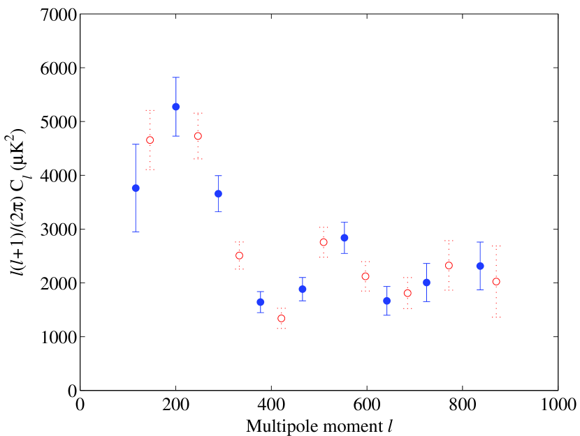
Figure 1: The angular power spectrum from the first season of DASI observations, plotted in nine bands (filled circles). We have analyzed the same data in nine bands shifted to the right (open circles). The alternate set of band powers are shown to demonstrate the robustness of the likelihood analysis procedure. To extract cosmological parameters (Paper III), only the nine bands shown in the primary analysis (filled circles) are used. Adjacent bands are anticorrelated at the 20% level (see Table 2). In addition to the uncertainties plotted above, there is a calibration uncertainty of 8%, expressed as a fractional uncertainty on the $C_{l}$ band powers (4% in $\Delta T/T$), which is completely correlated across all bands due to the combined flux scale and beam uncertainties.

In a separate analysis, we fit for the maximum likelihood value of an additional parameter, the temperature spectral index of the fluctuations, $\beta$, where $T\propto\nu^{\beta}$. Fitting a single spectral index for all nine bands, we find $\beta=-0.1\pm 0.2$ (1 $\sigma$), while fitting a separate spectral index for $l<500$ and $l>500$ yields $\beta=-0.2\pm 0.3$ and $0.0\pm 0.4$ respectively, indicating the fluctuation power is consistent with CMB.

Values and marginal uncertainties for the angular power spectrum in the primary nine bands are given in Table 1. The center and $e^{-1/2}$ widths of the bands are calculated using band-power window functions adapted from Knox (1999) which are plotted in Paper III. These are the relevant window functions for calculating the expectation value of the band power given a theoretical power spectrum. We give the ratio of the uncertainty due to sky sample variance to the uncertainty due to noise, $\sigma_{\mathrm{s}}/\sigma_{\mathrm{n}}$, estimated using the offset log-normal formalism of Bond, Jaffe, & Knox (2000). In their notation, $\sigma_{\mathrm{s}}/\sigma_{\mathrm{n}}$ is given by $\mathcal{C}_{B}/x_{B}$, where $\mathcal{C}_{B}$ is the band power estimate expressed as $l(l+1)C_{l}/(2\pi)$ and $x_{B}$ is proportional to the instrument noise contribution to the band-power uncertainty. These values may be used to estimate the non-Gaussianity in the band-power marginal likelihood distributions for parameter estimation calculations — asymmetric uncertainties due to non-Gaussianity are negligible for most of our band powers and we do not plot them here. We also tabulate the band-power correlation matrix (Table 2). All of the data products necessary for performing cosmological parameter estimation from this data are available at our website.

Table 1: Angular power spectrum band powers and uncertainties

$l_{\mathrm{eff}}$	$l_{\mathrm{l}}$	$l_{\mathrm{h}}$	$l(l+1)C_{l}/(2\pi)\ (\mu K^{2})$	$\sigma_{\mathrm{s}}/\sigma_{\mathrm{n}}$	$l(l+1)C_{l}^{\mathrm{E1-E2}}/(2\pi)\ (\mu K^{2})$
118	104	167	$3770\pm 820$	23.6	$-250\pm 160\hskip 28.90755pt$
203	173	255	$5280\pm 550$	31.6	$140\pm 120\hskip 28.90755pt$
289	261	342	$3660\pm 340$	18.7	$120\pm 120\hskip 28.90755pt$
377	342	418	$1650\pm 200$	7.3	$160\pm 140\hskip 28.90755pt$
465	418	500	$1890\pm 220$	4.3	$70\pm 240\hskip 28.90755pt$
553	506	594	$2840\pm 290$	4.0	$0\pm 300\hskip 28.90755pt$
641	600	676	$1670\pm 270$	2.3	$120\pm 420\hskip 28.90755pt$
725	676	757	$2010\pm 350$	1.7	$-90\pm 580\hskip 28.90755pt$
837	763	864	$2320\pm 450$	1.1	$-490\pm 850\hskip 28.90755pt$

The uncertainties listed above do not include flux scale and beam calibration uncertainties. The total combined calibration uncertainty is 8% (1 $\sigma$), expressed as a fractional uncertainty on the $C_{l}$ band powers (4% in $\Delta T/T$).

Table 2: Correlation coefficient matrix for the DASI band powers given in Table 1

$1$	$-0.243$	$0.0349$	$-5.87\times 10^{-3}$	$1.09\times 10^{-3}$	$-3.01\times 10^{-4}$	$-1.08\times 10^{-4}$	$-1.24\times 10^{-4}$	$-1.99\times 10^{-4}$
	$1$	$-0.182$	$0.0286$	$-6.65\times 10^{-3}$	$3.90\times 10^{-4}$	$-1.00\times 10^{-3}$	$-6.88\times 10^{-4}$	$-4.85\times 10^{-4}$
		$1$	$-0.196$	$0.0372$	$-8.84\times 10^{-3}$	$-1.61\times 10^{-3}$	$-2.82\times 10^{-3}$	$-2.74\times 10^{-3}$
			$1$	$-0.234$	$0.0334$	$-0.0149$	$-5.52\times 10^{-3}$	$-6.69\times 10^{-3}$
				$1$	$-0.193$	$0.0247$	$-0.0193$	$-8.22\times 10^{-3}$
					$1$	$-0.219$	$0.0394$	$-0.0200$
						$1$	$-0.275$	$0.0339$
							$1$	$-0.220$
								$1$

6.1 Consistency Tests

We perform three types of tests to check the consistency of the data: i) $\chi^{2}$ tests on the difference between two visibility data vectors constructed from observations of the same fields on the sky, ii) construction of a nine-band power spectrum of the epoch-differenced visibility data vector, to test for significant deviation from zero power, and iii) $\chi^{2}$ tests on the difference between two power spectra constructed from independent fields on the sky. In the second and third types of test, we increase the number of frequency channels which are combined in the data vector in order to reduce the computational time required to produce the power spectra. This increased data compression yields a power spectrum similar to the one reported above.

Of the three types of test, the first is the most powerful tool for detecting non-Gaussianity or incorrect estimates of the noise. The reduced $\chi^{2}$ statistic is

$$\chi^{2}/N=(\Delta_{1}-\Delta_{2})^{T}(C_{n1}+C_{n2}+C_{Cg})^{-1}(\Delta_{1}-\Delta_{2})/N,$$ (11)

where $\Delta_{1}$ and $\Delta_{2}$ are the two data vectors, $C_{n1}$ and $C_{n2}$ are the (diagonal) noise covariance matrices, $C_{Cg}$ is the same ground constraint matrix that is used in the power spectrum likelihood analysis, and $N=\mathrm{dim}\ \Delta-\mathrm{rank}\ C_{Cg}$ are the degrees of freedom. We split the visibilities between the two epochs of available observations for each field row, yielding $\chi^{2}/N=1.03$. This $\chi^{2}$ value is significant given the $N\sim 3\times 10^{4}$ degrees of freedom — it indicates that the noise may be slightly non-Gaussian. In fact, we see improvement of this statistic if we increase the severity of the lunar cuts, but the effect on the power spectrum is negligible. It may also indicate that we slightly underestimate the noise of the data. However, the uncertainties in all bands are dominated by sky sample variance, rather than instrument noise, making the power spectrum robust against a noise underestimate of this magnitude.

A power spectrum in nine bands was created from the epoch-differenced data vector, and tested for deviation from zero power using a $\chi^{2}$ statistic, with the result $\chi^{2}/N=9.5/9$, which is consistent within the 68% confidence interval. The band powers for the epoch-differenced power spectrum are given in Table 1.

We use a $\chi^{2}$ statistic to test the consistency between power spectra generated from each of the four field rows. The $\chi^{2}$ statistic is constructed from the difference between two power spectra which sample independent sky, $\chi^{2}=(\mathcal{D}_{1}-\mathcal{D}_{2})^{T}(P_{1}+P_{2})^{-1}(\mathcal{D}_{1}-\mathcal{D}_{2})$, where $\mathcal{D}_{1},\mathcal{D}_{2}$ are the band-power vectors and $P_{1},P_{2}$ are the band-power covariance (inverse Fisher) matrices. The non-Gaussianity of the DASI power spectrum uncertainties is small, which justifies using a $\chi^{2}$ statistic; we have tested its validity with Monte Carlo techniques on simulated data and have not found a significant deviation from a $\chi^{2}$ distribution. The resulting values, with format $\chi^{2}/N$ ($\chi^{2}$ cumulative distribution function percentile), are: $14.9/9$ (91%), $13.3/9$ (85%), $10.9/9$ (72%), $4.5/9$ (12%), $6.2/9$ (28%) and $3.7/9$ (7%) for the A–B, A–C, A–D, B–C, B–D, C–D differenced field row pairs, respectively. The power spectra of the four field rows are in reasonable agreement.

To test the efficacy of the point source constraints described in §5, we split the data in each field row between the four fields with the highest and four with the lowest detected point source flux, and we create two power spectra from the two sets of combined fields. The $\chi^{2}/N$ value for the difference between the two power spectra is $11.5/9$ (75%) indicating they are consistent within the 68% confidence interval.

Although point sources are the foreground of primary concern for DASI, constraint matrices are demonstrably effective in removing this point source power, and the consistency tests above show that the power spectra from sets of fields with very different point source flux contributions are in good agreement after the constraint matrix is applied.

6.2 Diffuse Foregrounds

Diffuse foregrounds are expected to be low in the region of the DASI fields at our observing frequency (see Paper I). To check this, we place limits on the contribution of diffuse foregrounds to the power spectrum by creating constraint matrices from foreground templates. The constraint matrix formalism is a powerful technique for placing limits on foregrounds with a known relative intensity distribution, since it allows for arbitrary scaling of the template amplitude and spectral index, without knowledge of these quantities at microwave frequencies. We create foreground images centered on each of the DASI fields from the cleaned IRAS 100 $\micron$ maps of Finkbeiner, Davis, & Schlegel (1999), cleaned 408 MHz Haslam survey maps (Haslam et al. 1981; Finkbeiner 2001), and H$\alpha$ maps (Gaustad et al. 2000; McCullough 2001). These images are converted to visibility template vectors with the DASI simulation software. We marginalize over modes in the data which match the templates using the constraint matrix formalism described in §5. We constrain an arbitrary template amplitude and spectral index for each DASI field. With the addition of all of these foreground constraints, the maximum change in a band power is 3.3%, with most bands changing by less than 1%.

The Haslam map has a resolution of $\sim 1\arcdeg$, making it inadequate as a template for multipole moments $\gtrsim 200$, however, the power spectrum of synchrotron emission is expected to decrease with $l$ (Tegmark & Efstathiou 1996). Also, the H$\alpha$ images show very low emission in the region of the DASI fields, and are of questionable use as a template. As a second method of characterizing possible free-free emission, we convert the H$\alpha$ images to brightness temperature at our frequencies assuming a gas temperature of $10^{4}$ K (Kulkarni & Heiles 1988). Subsequent power spectrum analysis of the resulting image visibility templates yields a $<1$% contribution to our band powers in all bands.

We conclude that dust, free-free, and synchrotron emission, as well as emission with any spectral index that is correlated with these templates, such as spinning dust grain emission (Draine & Lazarian 1998), make a negligible contribution to the CMB power spectrum presented here.

7 Conclusion

In its initial season, the Degree Angular Scale Interferometer has successfully measured the angular power spectrum of the CMB over the range $l$ = 100–900 in nine bands with high precision. The interferometer provides a simple and direct measurement of the power spectrum, with systematic effects, calibration methods, and beam uncertainties which are very different from single-dish experiments. We have made extensive use of constraint matrices in the analysis as a simple method for projecting out undesired signals in the data, including ground-signal common modes and point sources with arbitrary spectral index. The constraint matrix formalism is also used as a powerful test of correlations with foreground templates with arbitrary flux and spectral index scaling; we find no evidence of diffuse foregrounds in the data.

We see strong evidence for both first and second peaks in the angular power spectrum at $l\sim 200$ and $l\sim 550$, respectively, and a rise in power at $l\sim 800$ that is suggestive of a third. The detection of harmonic peaks in the power spectrum is a resounding confirmation that sub-degree scale anisotropy in the CMB is the result of gravitationally driven acoustic oscillations such as those which arise naturally in adiabatic inflationary theories. In addition, the rise in power in the region of the predicted third peak strongly supports, from CMB data alone, the presence of dark matter in the Universe.