Cosmological Parameter Extraction from the First Season of Observations with DASI

Abstract

The Degree Angular Scale Interferometer (DASI) has measured the power spectrum of the Cosmic Microwave Background anisotropy over the range of spherical harmonic multipoles $100<l<900$. We compare this data, in combination with the COBE-DMR results, to a seven dimensional grid of adiabatic CDM models. Adopting the priors $h>0.45$ and $0.0\leq\tau_{c}\leq 0.4$, we find that the total density of the Universe $\Omega_{tot}=1.04\pm 0.06$, and the spectral index of the initial scalar fluctuations $n_{s}=1.01^{+0.08}_{-0.06}$, in accordance with the predictions of inflationary theory. In addition we find that the physical density of baryons $\Omega_{b}h^{2}=0.022^{+0.004}_{-0.003}$, and the physical density of cold dark matter $\Omega_{cdm}h^{2}=0.14\pm 0.04$. This value of $\Omega_{b}h^{2}$ is consistent with that derived from measurements of the primeval deuterium abundance combined with big bang nucleosynthesis theory. Using the result of the HST Key Project, $h=0.72\pm 0.08$, we find that $\Omega_{tot}=1.00\pm 0.04$, the matter density $\Omega_{m}=0.40\pm 0.15$, and the vacuum energy density $\Omega_{\Lambda}=0.60\pm 0.15$. (All 68% confidence limits.)

1 Introduction

The angular power spectrum of the cosmic microwave background (CMB) has much to teach us about the nature of the Universe in which we live (Hu, Sugiyama, & Silk 1997). Measurements are improving rapidly (de Bernardis et al. 2000; Hanany et al. 2000; Padin et al. 2001), and for a wide variety of theoretical scenarios the predicted spectra can be calculated accurately (Zaldarriaga & Seljak 2000). Comparison of the data and models allows quantitative constraints to be placed on the parameters of the Universe in which we find ourselves, and is the subject of this paper.

The Degree Angular Scale Interferometer (DASI), along with its sister instrument the CBI (Padin et al. 2001) and the VSA (Jones 1996), is one of several new compact interferometers specifically designed for observations of the CMB. This paper is the third in a set of three. Paper I (Leitch et al. 2001) gives a detailed description of the instrument, observations, and data calibration. Paper II (Halverson et al. 2001) focuses on the extraction of the angular power spectrum from the calibrated interferometric data, and provides band-power estimates of the angular power spectrum of the CMB. In this paper we combine the low-$l$ measurements made by the COBE-DMR instrument (Bennett et al. 1996) with the new measurements from DASI to constrain the parameters of cosmological models.

The layout of this paper is as follows. The considerations which drive our selection of the model and parameter space to probe are detailed in §2. In §3 we review the method used to compare band power data to theoretical spectra. The results of this comparison are described in §4, and in §5 we draw some conclusions.

2 Models, Parameters and Model Grid Considerations

Following the discovery of the CMB, and the realization that the Universe went through a hot plasma epoch, it was proposed that adiabatic density perturbations in that plasma would lead to acoustic oscillations (Peebles & Yu 1970), and a series of harmonic peaks in the angular power spectrum (Doroshkevich, Zeldovich, & Sunyaev 1978). It was assumed that the initial fluctuations were scale invariant only because this is the simplest possible case. It was not until later that (New) Inflation was proposed (Guth & Pi 1982; Bardeen, Steinhardt, & Turner 1983; Hawking 1982; Starobinsky 1982) — an elegant cosmo-genic mechanism which naturally produces such conditions. The simplest versions of this theory also make the firm prediction that the Universe is exactly flat, i.e., has zero net spatial curvature.

Although Inflation sets the stage at the beginning of the plasma epoch it has nothing to say about the contents of the Universe. Over the last several decades a wealth of evidence has accumulated for the existence of some form of gravitating matter which does not interact with ordinary baryonic material; the so-called cold dark matter (CDM). Conflicting theoretical expectations and experimental measurements led to the proposal that a third component is present — an intrinsic vacuum energy. This three component model is the scenario we have chosen to consider.

The density required to produce zero net spatial curvature is referred to as the critical density $\rho_{c}=3H_{0}^{2}/(8\pi G)$, where $H_{0}$ is the Hubble constant ($H_{0}\equiv 100h$ km s^-1 Mpc^-1). It is convenient to measure the present day density of a component of the Universe in units of $\rho_{c}$, denoting this $\Omega_{i}$: the density of baryonic matter $\Omega_{b}$, the density of CDM $\Omega_{cdm}$, and the equivalent density in vacuum energy $\Omega_{\Lambda}$. Thus the density of matter is given by $\Omega_{m}\equiv\Omega_{b}+\Omega_{cdm}$ and the total density is given by $\Omega_{tot}\equiv\Omega_{m}+\Omega_{\Lambda}$. Since $\Omega_{i}=\rho_{i}/\rho_{c}$ note that $\Omega_{i}h^{2}$ is a physical density independent of the value of the Hubble constant.

To generate theoretical CMB anisotropy power spectra we have used version 3.2 of the freely available CMBFAST program (Zaldarriaga & Seljak 2000). This is the most widely used code of its type, and versions 3 and greater can deal with open, flat and closed universes. CMBFAST calculates how the initial power spectrum of density perturbations is modulated through the acoustic oscillations during the plasma phase, by the effects of recombination, and by reionization as the CMB photons stream through the Universe to the present. The program sets up transfer functions, taking as input $\Omega_{b}$, $\Omega_{cdm}$ and $\Omega_{\Lambda}$, as well as $H_{0}$, the optical depth due to reionization ($\tau_{c}$), and some other parameters. It can then translate initial perturbation spectra into the mean angular power spectra of the CMB anisotropy which would be observed in such a universe today. Inflation predicts that the initial spectrum is a simple power law with slope close to, but not exactly, unity.

In any given comparison of data to a multidimensional model we may have external information about the values of some or all of the parameters. This may come from theoretical prejudice, or from other experimental results. It may also be that the data set in hand is unable to simultaneously constrain all of the possible model parameters to the precision which we desire. In such cases we can choose to invoke our external knowledge, and fold additional information about the preferred parameter values into the likelihood distribution. Often this occurs because a parameter which could potentially be free is fixed at a specific value (an implicit prior). Or we may multiply the likelihood distribution by some function which expresses the values of the parameters which we prefer (an explicit prior). The choice of measure, e.g., whether a variable is taken to be linear or logarithmic, is also an implicit prior — although such distinctions become less important as a variable becomes increasingly well constrained.

There is no a priori reason to suppose that the marginal likelihoods of the cosmological parameters are Gaussian. Thus the curvature of the likelihood surface at the peak does not fully characterize the distribution. To set accurate constraints it is therefore necessary to explore the complete likelihood space by testing the data against a large grid of models. If the introduction of priors is to be avoided the grid must be expanded until one can be confident that it encompasses essentially all of the total likelihood.

Unfortunately it turns out that even within the paradigm of adiabatic CDM models the anisotropy power spectrum of the CMB does not fully constrain the parameters of the Universe. For example, it is well known that $\Omega_{m}$ and $\Omega_{\Lambda}$ are highly degenerate. It is always necessary to invoke external information in any constraint-setting analysis. The clear articulation of these priors, both implicit and explicit, is critically important, as has previously been noted (Jaffe et al. 2001).

We have chosen to consider a seven dimensional model space. The parameters which we include are the physical densities of baryonic matter ($\Omega_{b}h^{2}\equiv\omega_{b}$) and CDM ($\Omega_{cdm}h^{2}\equiv\omega_{cdm}$), as well as the spectral slope of the initial scalar fluctuations ($n_{s}$), and the overall normalization of the power spectrum as measured by the amplitude at the tenth multipole ($\mathcal{C}_{10}\equiv l(l+1)C_{10}/2\pi$). Noting that the degeneracy in the $(\Omega_{m},\Omega_{\Lambda})$ plane is along a line of constant total density we opt to rotate the basis vectors by 45^∘ and grid over the sum and difference of these parameters: $\Omega_{m}+\Omega_{\Lambda}\equiv\Omega_{tot}$ and $\Omega_{m}-\Omega_{\Lambda}\equiv\Omega_{\Delta}$. This reduces the size of the model grid required to box in the region of significant likelihood. The seventh parameter is the optical depth due to reionization ($\tau_{c}$). Note that for each point in $(\Omega_{\Delta},\Omega_{tot},\omega_{b},\omega_{cdm})$ space there is an implied value of the Hubble constant ($h=\sqrt{2(\omega_{b}+\omega_{cdm})/(\Omega_{tot}+\Omega_{\Delta})}$) so we can calculate the $(\Omega_{b},\Omega_{cdm},\Omega_{\Lambda},h)$ values for input to CMBFAST.

We assume, as is the theoretical prejudice, that the contribution of tensor mode perturbations is very small as compared to scalar, and ignore their effect (Lyth 1997). Tensor modes primarily contribute power at low $l$ numbers, so if a large fraction of the power seen by DMR were caused by this effect the scalar spectrum would need to be strongly tilted up to provide the observed power at smaller angular scales. However we know that $n_{s}$ cannot be $\gg 1$ as this would conflict with results from large scale structure studies. Our constraints should, however, be taken with an understanding of our assumption regarding tensor modes.

In principle some of the dark matter could be in the form of relativistic neutrinos (hot as opposed to cold dark matter). However the change that this would make to the CMB power spectrum is negligible compared to the uncertainties of the DASI data (Dodelson, Gates, & Stebbins 1996). We therefore assume that all the dark matter is cold, and set $\Omega_{\nu}=0$, although it should then be understood that the $\Omega_{cdm}h^{2}$ value we find may, in principle, contain some hot dark matter.

Papers fitting the BOOMERANG-98 and MAXIMA-1 band-power data (Balbi et al. 2000; Lange et al. 2001; Jaffe et al. 2001) considered seven dimensional grids rather similar to our own. Other studies have examined model grids with as many as 11 dimensions (Tegmark, Zaldarriaga, & Hamilton 2001), including an explicit density in neutrinos and tensor mode perturbations, generally finding both effects to be small.

Taking the philosophy that simplicity is a virtue, we have not made use of $l$-space or $k$-space splitting to accelerate the calculation of the model grid (Tegmark et al. 2001). In addition we have generated a simple regular grid, rather than attempting to concentrate the coverage in the maximum likelihood region. Finally we have not treated the normalization parameter $\mathcal{C}_{10}$ as continuous, preferring to explicitly grid over this parameter as well. This is computationally somewhat slower, but makes the marginalization simpler, and involves no assumption about the form of the variation of $\chi^{2}$ versus this parameter. Using the notation lower-edge:step-value:upper-edge (number-of-values) our grid is as follows: $\Omega_{\Delta}=-1.0:0.2:3.4$ (23), $\Omega_{tot}=0.7:0.05:1.3$ (13), $\Omega_{b}h^{2}=0.0100:0.0025:0.0400$ (13), $\Omega_{cdm}h^{2}=0.00:0.05:0.5$ (11), $\tau_{c}=0.0:0.1:0.4$ (5), $n_{s}=0.75:0.05:1.25$ (11), and $\mathcal{C}_{10}=300:50:1300$ (21). Excluding the small, physically unreasonable corner of parameter space where $\Omega_{m}\leq 0$, we make $205,205$ runs of CMBFAST generating $205,205\times 11=2,257,255$ theoretical spectra and calculating $2,257,255\times 21=47,402,355$ values of $\chi^{2}$ against the data.

For theoretical and phenomenological discussions of how the various peak amplitudes and spacings of the power spectrum are related to the model parameters see Hu et al. (1997) and Hu et al. (2001). In this paper we choose to compare data and models without explicitly considering such connections.

3 Comparison of Data and Models

Consider a set of observed band-powers $\mathcal{D}_{i}$ in units of $\mu$K², together with their covariance matrix $P_{ij}$. If the overall fractional calibration uncertainty of the experiment is $s$ we can add this to the covariance matrix as follows:

$$N_{ij}=P_{ij}+s^{2}\mathcal{D}_{i}\mathcal{D}_{j}.$$ (1)

For the purposes of the present analysis we assume $s=0.08$ which includes both temperature scale and beam uncertainties (the fractional error on the band-powers is 8% corresponding to 4% in temperature units — see Paper II).

Now consider a model power spectrum $\mathcal{C}_{l}$. The expectation value of the data given the model is obtained through the “band-power” window function $W^{\mathrm{B}}_{il}/l$ (Knox 1999),

$$\mathcal{T}_{i}=\sum_{l}\mathcal{C}_{l}\frac{W^{\mathrm{B}}_{il}}{l}.$$ (2)

The band-power window functions $W^{\mathrm{B}}_{il}/l$ are calculated from the band-power Fisher matrix, $F$, and the Fisher matrix $F^{\mathrm{s}}$ of the bands, $b_{i}$, sub-divided into individual multipole moments,

$$\frac{W^{\mathrm{B}}_{il}}{l}=\sum_{i^{\prime}}{\left(F^{-1}\right)}_{ii^{\prime}}\sum_{l^{\prime}\in b_{i^{\prime}}}F^{\mathrm{s}}_{ll^{\prime}},$$ (3)

(adapted from Knox 1999, for Fisher matrices with significant off-diagonal elements). The sum of each row of the array $W^{\mathrm{B}}_{il}/l$ is unity, so Equation (2) simply represents a set of weighted means. Note that any experiment with less than full sky coverage will always have non top-hat band-power window functions. In practice, we calculate Equation (3) by subdividing each band into four sub-bands, and interpolate the results. The functions for the DASI band-powers are plotted in Figure 1, and are available at our website. In practice the effect of using the correct window function, versus simply choosing the $\mathcal{C}_{l}$ at the nominal band center, is extremely modest.

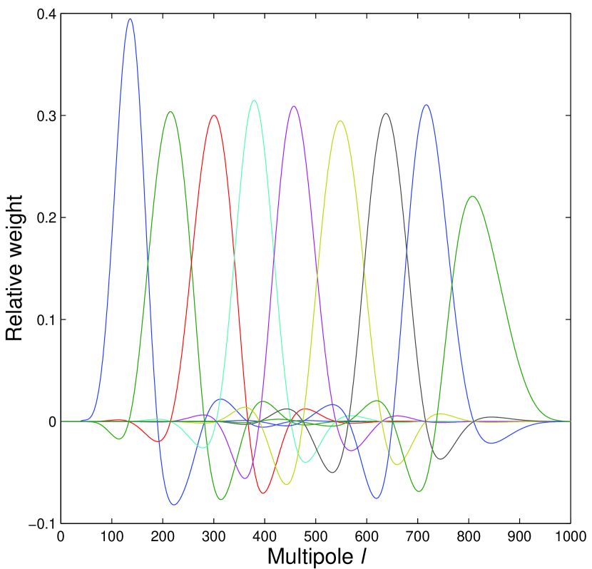
Figure 1: Window functions for the DASI band-powers.

The uncertainties of the $\mathcal{D}_{i}$ are non-Gaussian so it would not be correct to calculate $\chi^{2}$ at this point. However it is possible to make a transformation such that the uncertainties become Gaussian to a very good approximation (Bond, Jaffe, & Knox 2000). An additional set of quantities $x_{i}$ need to be calculated from the data which represent the component of the total uncertainty which is due to instrument noise. We can then transform each of the variables as follows,

$$\mathcal{D}_{i}^{Z} = \ln(\mathcal{D}_{i}+x_{i})$$ (4)

$$\mathcal{T}_{i}^{Z} = \ln(\mathcal{T}_{i}+x_{i})$$ (5)

$$M_{ij}^{Z} = N_{ij}^{-1}(\mathcal{D}_{i}+x_{i})(\mathcal{D}_{j}+x_{j}),$$ (6)

and calculate $\chi^{2}$ as usual,

$$\chi^{2}=(\mathcal{D}_{i}^{Z}-\mathcal{T}_{i}^{Z})M_{ij}^{Z}(\mathcal{D}_{j}^{Z}-\mathcal{T}_{j}^{Z}).$$ (7)

The inverse covariance matrix elements $M^{Z}_{ij}$ will be approximately independent of the bandpowers $\mathcal{D}_{i}$. This is true even with the added calibration uncertainty term in Equation (1), under the assumption that the band-power uncertainty is sample variance dominated, i.e., $\mathcal{D}_{i}/x_{i}\gg 1$ (as is the case with almost all the DASI band-powers), or that the fractional calibration uncertainty is small compared to the total uncertainty in the band-power, $s^{2}\ll N_{ii}/\mathcal{D}_{i}^{2}$, which is the case for DMR. Use of this transformation is very important as it allows us to use $\chi^{2}$, and therefore not only to find the best fitting model, but to determine an absolute goodness of fit.

The ability of smaller angular scale ($l>100$) CMB data to set constraints on model parameters is much improved when the large angular scale ($l\leq 25$) information from the DMR instrument is included. We use the DASI bandpowers described and tabulated in Paper II together with the 24 DMR band-powers provided in the RADPACK distribution (Knox 2000; Bond et al. 2000), concatenating the $\mathcal{D}_{i}$ and $x_{i}$ vectors and forming a block diagonal covariance matrix. Note that while the effect of the transformation described above is modest for the DASI points, it is very important for those from DMR (due to the large sample variance at the lower $l$’s).

4 Results

Figure 2 shows the DASI band-powers, together with the DMR data condensed to a single point for display. The $\chi^{2}$ of the best fit model which falls on our grid is $29.5$ for the 9 DASI plus 24 DMR band-powers. Assuming a full 7 degrees of freedom are lost to the fit, this is at the 71% point of the cumulative distribution function (cdf). The parameters of this model are $(\Omega_{m},\Omega_{\Lambda},\Omega_{b}h^{2},\Omega_{cdm}h^{2},\tau_{c},n_{s},\mathcal{C}_{10})=(0.725,0.325,0.0200,0.15,0.0,0.95,800)$, equivalent to $(\Omega_{b},\Omega_{cdm},\Omega_{\Lambda},\tau_{c},n_{s},h)=(0.09,0.64,0.33,0,0.95,0.48)$. However, no particular importance should be ascribed to these — the concordance model (Ostriker & Steinhardt 1995; Krauss & Turner 1995) which is shown has a $\chi^{2}$ of 30.8 (76%) and is also rather a good fit. The message of Figure 2 is simply that there are models within the grid which fit acceptably well, and that we are therefore justified in proceeding to marginalized parameter constraints. We convert $\chi^{2}$ to likelihood, $\mathcal{L}=e^{-\chi^{2}/2}$.

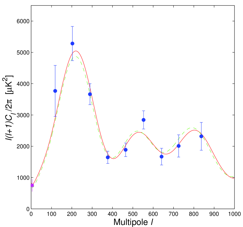
Figure 2: The DASI first-season angular power spectrum in nine bands (closed circles). The DMR information is shown compressed to the single lowest $l$ point. The solid (red) line is the best fitting model which falls on our grid, while the dashed (green) shows the concordance model $(\Omega_{b},\Omega_{cdm},\Omega_{\Lambda},\tau_{c},n_{s},h)=(0.05,0.35,0.60,0,1.00,0.65)$. The error bars plotted here are strictly for illustrative purposes only. The $\chi^{2}$ calculation is made using the full covariance matrix, and after the transformation described in §3. Thus “Chi-by-eye” can be misleading.

The extreme degeneracy of CMB data in the $(\Omega_{m},\Omega_{\Lambda})$ plane has already been mentioned. This inability to choose between models with the same $\Omega_{tot}$ is in fact weakly broken at very low-$l$ numbers by the Sachs-Wolfe effect (Efstathiou & Bond 1999). The likelihood contours diverge from the $\Omega_{tot}=1$ line as $\Omega_{\Delta}$ becomes $\gg 1$, and the allowed region broadens. Consequently the marginal likelihood curve of $\Omega_{tot}$ acquires a high side tail as models with progressively greater $\Omega_{\Delta}$ are included. These high $\Omega_{\Delta}$ models have very low values of $h$, and are known to be invalid from a wide range of non-CMB data. This being the case it is clearly not sensible to allow them to influence our results.

We are therefore prompted to introduce additional external information. We could simply restrict $\Omega_{m}$ and $\Omega_{\Lambda}$ to some “reasonable” range; for example requiring $\Omega_{\Lambda}>0$ and $\Omega_{m}<1$. Instead we choose to introduce a prior on $h$ since this strongly breaks the degeneracy and is a quantity which is believed to have been measured to 10% precision (Freedman et al. 2000). We use two $h$ priors; a weak $h>0.45$, and a strong $h=0.72\pm 0.08$ assuming a Gaussian distribution. For the weak prior adding the additional restriction $h<0.90$ has almost no effect as the excluded models already have very small likelihoods. To apply the prior we simply calculate the $h$ value at each grid point, assign it the relevant likelihood, and multiply the two grids together.

Figure 3 shows how the marginal likelihood distributions of the model parameters change as we move from the implicit prior of $(\Omega_{\Delta}\leq 3.4,\Omega_{tot}\leq 1.3)$, to weak, and then strong prior cases. Note that most of the curves fall to a small fraction of their peak value before the edge of the grid is reached. For all parameters where this is not the case one must introduce external priors such that it becomes so, and/or acknowledge the implicit top-hat prior which the range of that grid parameter represents — only then can the constraint on any of the parameters be accepted. All such priors must then be quoted with the constraints. In fact we see that $(\Omega_{b}h^{2},\Omega_{cdm}h^{2},n_{s},\mathcal{C}_{10})$ are almost completely unaffected by the choice of prior on $h$ — this indicates that correlations between these parameters and $(\Omega_{\Delta},\Omega_{tot})$ are modest, and is a fortunate result.

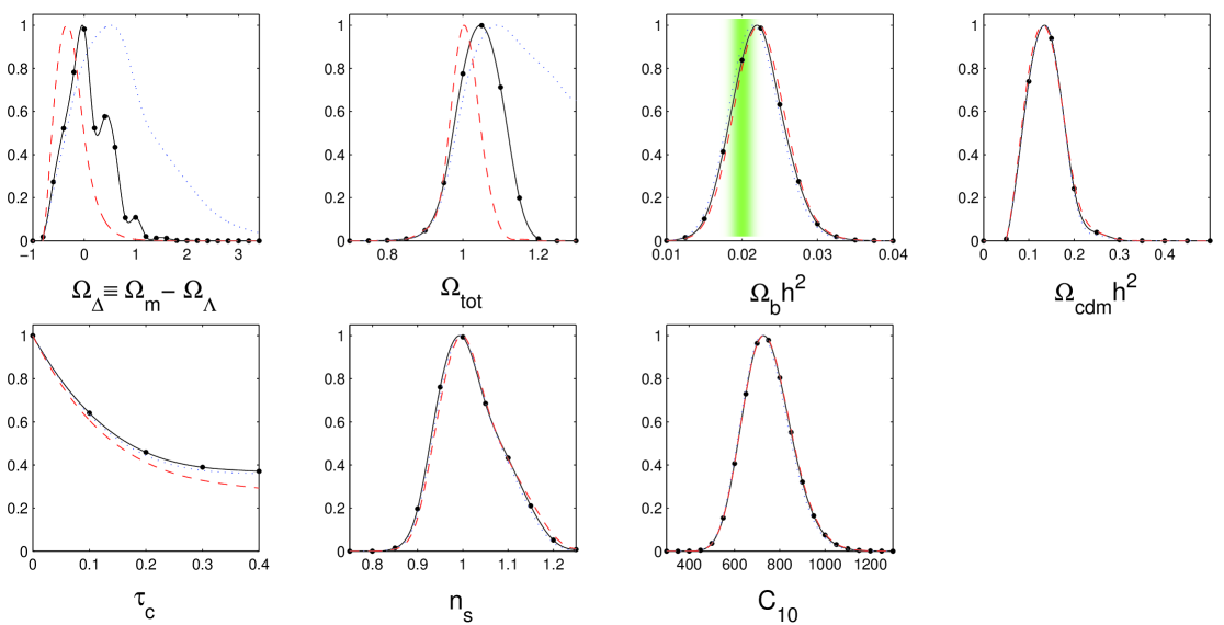
Figure 3: Marginal likelihood distributions for each dimension of the model grid. The dotted (blue) and solid (black) lines show the distribution before and after the introduction of a weak prior on the Hubble parameter ($h>0.45$). The dashed (red) lines shows the effect of the stronger prior $h=0.72\pm 0.08$. In the $\Omega_{b}h^{2}$ panel the BBN constraint is shown as a (green) shaded region. All curves are normalized to a peak height of unity, and are spline interpolations of the actual model grid values shown by the points.

We turn now to $\tau_{c}$ which, as is evident in Figure 3, is a very poorly constrained parameter. The effect of reionization is to suppress power at small angular scales, and tilt the spectrum down. However this can be compensated by adjusting $n_{s}$ upwards making these two parameters largely degenerate. Worse still, unlike the $h$ prior discussed above, we have very weak experimental guidance as to the value of $\tau_{c}$ — we know only that reionization occurred at $z\geq 6$, roughly equivalent to $\tau_{c}\geq 0.03$. From theoretical ideas regarding early structure formation, and energy emission, it seems essentially impossible that $\tau_{c}>0.4$ (see Haiman & Knox 1999, for a recent review of our knowledge regarding reionization). The theoretical prejudice for $n_{s}\approx 1$ is strong, but since this is a fundamental parameter of the cosmology which we are trying to measure, we are very reluctant to place a prior on it.

We have opted to accept the top-hat prior implicit in our model grid, i.e., that the likelihood of $\tau_{c}$ falling between 0.0 and 0.4 is uniform. In Table 1 we list the spline interpolated median, $1\sigma$ and $2\sigma$ points of the integral constraint curves. The modal (maximum likelihood) value is also given. All of the constraints quoted in this paper are 68% confidence intervals about the median. Although one can argue that the mode is perhaps more natural, in practice it makes little difference.

Table 1: Parameter constraints from DASI+DMR data

Parameter	2.5%	16%	50%	84%	97.5%	mode
$\Omega_{tot}$	0.927	0.986	1.044	1.103	1.150	1.047
$\Omega_{b}h^{2}$	0.0156	0.0187	0.0220	0.0255	0.0292	0.0220
$\Omega_{cdm}h^{2}$	0.075	0.100	0.137	0.175	0.225	0.135
$n_{s}$	0.901	0.949	1.010	1.092	1.166	0.993
$\mathcal{C}_{10}$	558	642	741	852	973	728

These constraints are from a seven dimensional grid, assuming the weak prior $h>0.45$, and $0.0\leq\tau_{c}\leq 0.4$. The indicated points on the cumulative distribution function are given, as well as the maximum likelihood value.

Referring to Figure 3 we see that the $\Omega_{\Delta}$ constraint is almost wholly driven by the prior on $h$; for this reason we have not included it in table 1. However, if one is prepared to accept the strong prior $h=0.72\pm 0.08$, then our data indicates that $\Omega_{tot}=1.00\pm 0.04$, $\Omega_{m}=0.40\pm 0.15$ and $\Omega_{\Lambda}=0.60\pm 0.15$.

Figure 4 illustrates the effect of setting $\tau_{c}=0.0$ (which the data weakly prefers). As already mentioned the primary degeneracy is with $n_{s}$ which shifts to $n_{s}=0.97^{+0.05}_{-0.04}$.

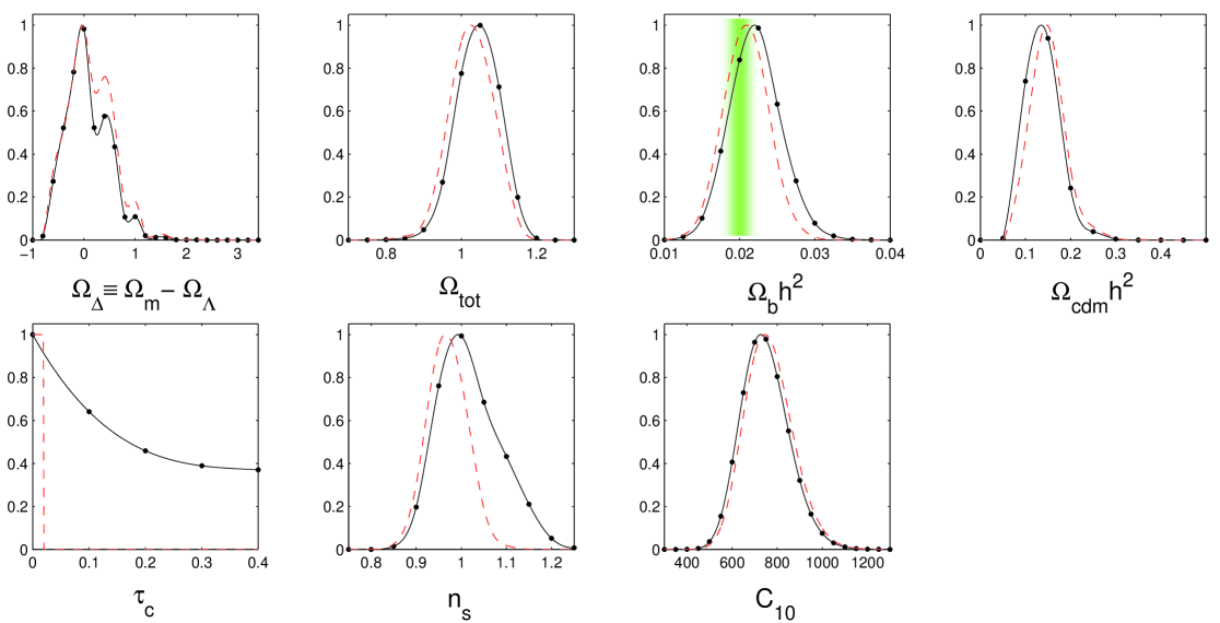
Figure 4: Marginal likelihood distributions when varying the prior on $\tau_{c}$. All curves assume the weak prior $h>0.45$. The solid (black) are the same as in Figure 3 and assume $0.0\leq\tau_{c}\leq 0.4$, while the dashed (red) set $\tau_{c}=0.0$.

The selection of the particular set of nine bandpowers which we have used in this analysis is quite arbitrary. We have tested increasing the number of bins — as expected the variance and covariance of the points increases to compensate, and the constraint curves remain the same. Shifting the bins in $l$ also leaves the results unchanged — for instance the alternate binning shown in Paper II leads to results which are indistinguishable from those presented here.

5 Conclusion

We have compared the DASI+DMR data to adiabatic CDM models with initial power law perturbation spectra. The best fitting model has an acceptable $\chi^{2}$ value, indicating that for data of the present quality models within this class are a plausible representation of the underlying physics. Adopting the conservative priors $h>0.45$ and $0.0\leq\tau_{c}\leq 0.4$, we find $\Omega_{tot}=1.04\pm 0.06$ and $n_{s}=1.01^{+0.08}_{-0.06}$, consistent with the predictions of Inflation. Moving to more aggressive priors on $h$ and $\tau_{c}$ tightens the constraints on $\Omega_{tot}$ and $n_{s}$ respectively but they remain consistent with the theory.

We find that $\Omega_{b}h^{2}=0.022^{+0.004}_{-0.003}$ and $\Omega_{cdm}h^{2}=0.14\pm 0.04$, adding to the already very strong evidence for non-baryonic dark matter. These constraints are only weakly affected by the choice of $h$ and $\tau_{c}$ priors. Setting a strong $h$ prior breaks the $(\Omega_{m},\Omega_{\Lambda})$ degeneracy such that we constrain $\Omega_{m}=0.40\pm 0.15$ and $\Omega_{\Lambda}=0.60\pm 0.15$— consistent with other recent results.

The current best value for $\Omega_{b}h^{2}$ derived from the well developed theory of big bang nucleosynthesis (BBN), combined with measurements of the primeval deuterium abundance, is $\Omega_{b}h^{2}=0.020\pm 0.002$ (Burles, Nollett, & Turner 2001, 95% confidence). The $\chi^{2}$ of the difference between this and our own value is at the 42% point of the cdf (assuming Gaussian errors on both); the values are hence consistent. Previous CMB analyses have seen little power in the second peak region, and have determined $\Omega_{b}h^{2}$ values higher than, and inconsistent with, BBN at the $\approx 3\sigma$ level (Lange et al. 2001; Jaffe et al. 2001).