Experiment Design and First Season Observations with the Degree Angular Scale Interferometer

Abstract

We describe the instrumentation, experiment design and data reduction for the first season of observations with the Degree Angular Scale Interferometer (DASI), a compact microwave interferometer designed to measure anisotropy of the Cosmic Microwave Background (CMB) on degree and sub-degree scales ($l\simeq$ 100–900). The telescope was deployed at the Amundsen-Scott South Pole research station during the 1999–2000 austral summer and conducted observations of the CMB throughout the following austral winter. In its first season of observations, DASI has mapped CMB fluctuations in 32 fields, each $3\fdg 4$ across, with high sensitivity.

1 Introduction

The use of the CMB angular power spectrum to constrain cosmological parameters has been the subject of much recent literature (see, e.g., Hu & White 1996, for a discussion of salient features of the power spectrum). We are at a point where the ability to resolve fine-scale structure in the power spectrum is no longer limited primarily by detector sensitivity, but by experiment design, understanding of calibration uncertainties and careful control of systematics. The comparison of complementary measurements by experiments of radically different design will prove critical to an understanding of what exactly the CMB is telling us.

Because they directly sample Fourier components of the sky, interferometers are uniquely suited to measurement of the CMB power spectrum and offer a completely independent technique, free of many of the systematics which must be carefully controlled in scanning experiments. The Degree Angular Scale Interferometer (DASI), along with its companion instrument the CBI (Pearson et al. 2000), and the VSA (Jones 1996), is one of a new generation of ultra-compact microwave interferometers designed to measure anisotropy in the CMB. With 13 elements operating in ten 1-GHz bands from 26–36 GHz, DASI provides dense sampling of the power spectrum from $l=100$ to $l=900$, angular scales spanning the first three harmonically related acoustic peaks in $\Omega\sim 1$ cosmologies.

This paper describes details of the instrument, design of the experiment, and calibration and reduction of the Fourier-plane visibility data. Analysis of these data and extraction of the angular power spectrum are presented in Halverson et al. (2001, hereafter Paper II), while limits on cosmological parameters from the DASI data are given in Pryke et al. (2001, hereafter Paper III).

In sections §2 and §3 of this paper, we discuss details of the instrument design. A description of the site is given in §4. We discuss foregrounds in §5. The CMB observations are described in §6 and §7. Data reduction and analysis are presented in §8 and §9, and results are presented in §10.

2 Instrument

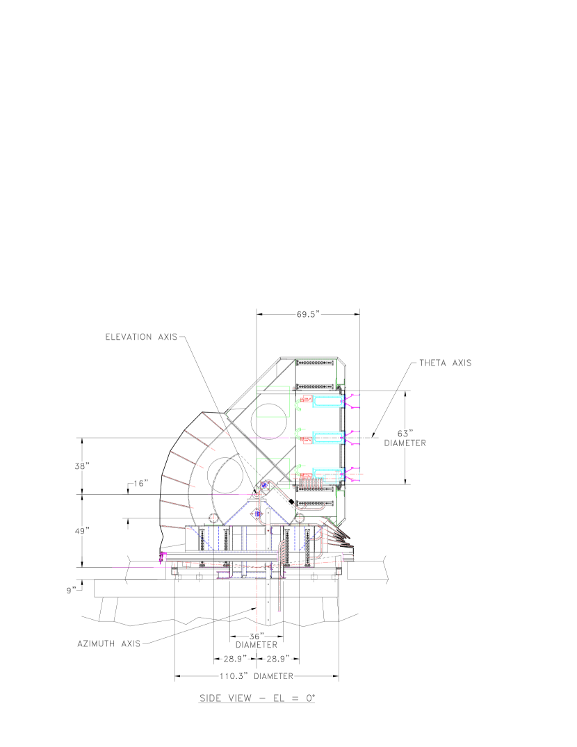
Figure 1: Schematic of the DASI telescope. Shown is a side view of the instrument, at EL = 0, with the faceplate pointing to the right.

2.1 Telescope Mount

The telescope is situated atop the inner of two concentric towers attached to the Martin A. Pomerantz Observatory (MAPO), 0.7 km from the geographic South Pole. The inner tower is mechanically isolated from the outer tower to minimize vibrations transmitted from the building to the telescope. Although diurnal variations in the ambient temperature at the Pole are extremely small (see §4), the legs of the inner tower are insulated to minimize tilt of the azimuth ring from differential thermal expansion by direct solar heating during the summer months.

A room beneath the telescope, attached to the outer tower, houses helium compressors, drive amplifiers, and an air handling unit for managing waste heat from the telescope and compressors. The interior of the telescope opens directly onto the compressor room, providing access to drive systems, receivers and electronics even in mid-winter, when the darkness and extreme cold (as low as $-80\arcdeg$ C ambient) severely restrict outside activity. An insulated fabric bellows permits motion in the elevation axis while maintaining the interior of the telescope and drive assemblies at room temperature using only waste heat from the telescope systems. Tested for flexibility to $-100\arcdeg$ C, the bellows has thus far functioned perfectly at polar temperatures.

The telescope mount is an altitude-azimuth design, employing a counterbalanced gear and pinion elevation drive, for tracking and pointing stability. Heavy box steel construction lends the mount extreme rigidity and immunity to flexure; the combined weight of the telescope, when fully equipped and operational, is approximately 35,000 lbs.

The absolute pointing of the telescope is derived from observations of bright stars made with a small optical camera mounted on the faceplate. In an automated procedure, approximately 80 positions for stars distributed throughout the sky are acquired using a frame grabber. These observations are fit with an eight parameter pointing model, yielding $\sim 20^{\prime\prime}$ rms residuals. Limits on the deviation of the radio pointing from this model are discussed in §9.

2.2 Faceplate

The interferometer has 13 primary antenna elements, arranged in a three-fold symmetric pattern on a rigid faceplate attached to the elevation cradle. The locations of the antennas in the faceplate were numerically optimized to provide nearly uniform sampling over the multipole range probed by DASI, $l\sim 100$–900 (see Figure 2). The rigid faceplate greatly simplifies the design of the correlator, since unlike conventional tracking arrays, projected baseline lengths for a co-planar array are independent of the pointing center, and tracking delays are not required.

The faceplate can also be rotated about its axis. In combination with the three-fold symmetry, this feature provides important diagnostic capabilities, for instance permitting discrimination of spurious signals due to cross-talk between the antenna elements. Since the antenna pattern repeats with every $120\arcdeg$ of rotation, any signal in the far-field remains unchanged by such a rotation; signals due to cross-talk, however, will rotate with the faceplate. Moreover, at the South Pole, celestial sources track at fixed elevation, and the ability to simulate parallactic angle rotation provides a powerful consistency check for observations of calibrator sources, as described in §7.2. For purposes of imaging, the rotation also allows dense sampling of the Fourier plane (see §3).

2.3 Primary Antenna Elements

Each antenna consists of a 20-cm aperture, $30\arcdeg$ semi-flare angle corrugated horn with a lens to correct the phase front and achieve a diffraction-limited beam on the sky. To make the array maximally compact, the receiver dewars were designed to fit entirely within the footprint of the horns; the shortest baseline is $25.1$ cm. Unlike Cassegrain elements, horns provide unobstructed apertures, with lower sidelobe response and better cross-talk characteristics, important for a compact array in which the elements are nearly touching. Each antenna element is further surrounded by a corrugated shroud, yielding a measured monochromatic crosstalk level of less than $-100~{}{\rm dB}$ in laboratory measurements of the horn-lens combination (Halverson & Carlstrom 2001). To further suppress cross-talk from correlated amplifier noise, the receivers are also equipped with front-end isolators.

Each element is equipped with a high density polyethylene lens, resulting in a high aperture efficiency, $83.5\%$, and permitting an extremely compact horn design. At polar temperatures, the lens contributes less than $2.5~{}{\rm K}$ to the system temperature.

The beam pattern, which determines the field of view of the interferometer, has been characterized in range measurements at 26, 30 and 36 GHz and in each case found to agree closely with the predicted pattern, both in the sidelobe response, which is typically $-20~{}{\rm dB}$ at the first sidelobe, and in the main beam width, which is $3\fdg 4$ FWHM at 30 GHz (Halverson & Carlstrom 2001). From the agreement between these measurements and the theoretical beam pattern, we adopt the theoretical value as our estimate of the true aperture efficiency and assign a fractional uncertainty of $4\%$, as shown in Table 1.

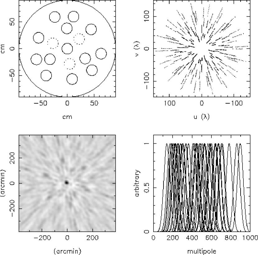
Figure 2: Top left: The DASI faceplate configuration. Solid circles represent locations of the 13 antennas. (Dashed circles are additional faceplate slots.) Top right: The resulting instantaneous Fourier plane coverage of the interferometer, showing radial extension due to the frequency dependence of the $(u,v)$ coordinates. Bottom left: one of the brightest point sources in the DASI fields, showing the synthesized beam pattern. Radial features in the image are artifacts of the sampling. Bottom right: The effective $l$-space window functions of the 26 distinct DASI baselines, shown for 26.5 and 35.5 GHz. Note that this represents only 1/5 of DASI’s instantaneous $l$-space sampling.

2.4 Signal Chain

Each receiver employs a cryogenically cooled, 4-stage InP HEMT amplifier operating from 26–36 GHz. These amplifiers were constructed at the University of Chicago, after a design developed at NRAO (Pospiezalski et al. 1995). Receiver temperatures range from 15–26 K at the center of the band, increasing to an average of $30~{}{\rm K}$ at the band edges. These noise temperatures include the HEMTs, isolator and polarizer (all at 10 K), and warm throat, horn and lens. Including CMB and atmosphere, we achieve typical system temperatures of 26 K at band center, for an rms sensitivity per visibility of approximately $60~{}{\rm Jy~{}s^{1/2}}$ in a 1 GHz band.

The 26–36 GHz RF signal from each antenna is mixed down to 2–12 GHz IF band using a local oscillator (LO) tuned to $38$ GHz. The IF signal is split into ten 1-GHz wide bands, each of which is further mixed down to 1–2 GHz. The 13 signals at each frequency are fed to one of 10 identical analog correlators (Padin et al. 2001), where the 78 complex multiplications are formed, digitized and integrated for 0.84 s in a digital accumulator. A copy of each input signal is phase-shifted by $90\arcdeg$, and multiplications are performed simultaneously for the real and imaginary Fourier components. A $180\arcdeg$ phase switch is applied to each LO in a Walsh sequence on a $25.6~{}{\rm\mu s}$ clock interval and is demodulated by the accumulators, to remove any offsets or slowly varying pickup. To further reduce residual offsets, a second, slower level of $180\arcdeg$ Walsh switching is applied to the LOs, and is demodulated in software with a switching period equal to the readout interval. The multiplier gains and quadrature errors are periodically calibrated by injection of a correlated broadband noise source at the input to each receiver.

Each analog correlator is integrated onto a single full-depth VME card, and the entire 10 GHz correlator fits into a crate approximately 75 cm on a side. Filtering and down-conversion of the IF signal is accomplished in a similar crate, and both rotate with the antennas on the underside of the telescope faceplate. The short fixed distance from the receivers to the downconverter and correlator eliminates flexure of cables carrying phase-sensitive signals, resulting in excellent phase stability; observed instrumental phase drifts are less than $10\arcdeg$ over a period of many weeks.

3 Interferometer Characteristics

An interferometer directly measures components of the Fourier transform of the sky brightness. The response on the sky for a two-element interferometer is an interference fringe pattern, with the sinusoidal variation oriented parallel to the baseline vector b connecting the two elements. The spacing of the fringe pattern is ${\lambda/b}$, where $\lambda$ is the observing wavelength and $b$ is the magnitude of the projection of b perpendicular to the line of sight. Each baseline of a multi-element array therefore probes a point $\mathbf{u}$ in Fourier space whose coordinates are given by $(u,v)=(b_{x}/\lambda,b_{y}/\lambda)$, or in terms of multipole moment, $l\simeq 2\pi b/\lambda$ (for $l\gtrsim 60$) (White et al. 1999); shorter baselines measure larger angular scales, and vice versa.

The fringe pattern on the sky is enveloped by the primary beam of the array elements, $A(\mathbf{x},\lambda)$, where $\mathbf{x}$ is a direction on the sky. The output of the interferometer, the visibility, is the time-averaged integral of this pattern, multiplied by the sky brightness, and is the fundamental data quantity discussed in these papers. For observations of the CMB in the Rayleigh-Jeans limit, the visibility in the flat-sky approximation is given by

$$V(\mathbf{u})=\frac{2k_{B}T}{\lambda^{2}}\int^{\infty}_{-\infty}{d{\mathbf{x}\,A(\mathbf{x},\lambda)\frac{{\Delta T}}{T}(\mathbf{x})e^{-2\pi i\mathbf{u\cdot x}}}}.$$ (1)

Since the CMB power spectrum is directly related to the Fourier transform of the brightness $\widetilde{\Delta T}(\mathbf{u})$,

$$C_{l}\Big{|}_{l=2\pi|\mathbf{u}|}\simeq\left<\left|\frac{\widetilde{\Delta T}}{T}(\mathbf{u})\right|^{2}\right>,$$ (2)

appropriate for $|\mathbf{u}|\gtrsim 10$ (White et al. 1999), a simple estimator for the $C_{l}$ can be constructed from the variance of the visibilities (see Paper II for a more formal discussion).

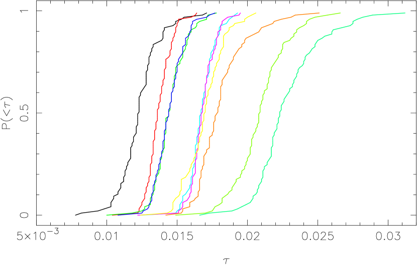
Figure 3: Cumulative opacity distributions, by frequency, at the South Pole, from 05 May–07 November 2000. The ten curves in this plot, from left to right, are for frequencies from 26.5 to 35.5 GHz in 1 GHz steps.

With 13 elements, the DASI array yields 78 distinct baseline vectors; the frequency dependence of the $(u,v)$ coordinates means that with 10 frequency channels, DASI samples 780 different points in the Fourier plane (see Figure 2), although visibilities from neighboring frequencies of the same baseline are highly correlated. The 3-fold symmetry of the faceplate reduces the number of unique baseline lengths to 26, each pointing of the telescope producing 3 independent measurements of the same multipole at each frequency. With baseline separations ranging from 25.1–120.7 cm, DASI samples multipole moments from $l=140$ at the lowest frequency to $l=900$ at the highest. Array parameters are summarized in Table 1.

Images of the sky can be produced from an interferometer by simple Fourier inversion of the visibilities. The transform of the $(u,v)$ sampling defines the effective resolution of the image, the so-called synthesized beam; for DASI, the instantaneous $(u,v)$ coverage produces a synthesized beam width of approximately $20^{\prime}$ (FWHM), with radial sidelobes due to the radial structure of the $(u,v)$ sampling (top right of Figure 2).

Rotation of the faceplate preserves the baseline lengths, but rotates the fringe patterns on the sky. This feature can be used to obtain additional independent samples of the same multipole moment in a given field, or for purposes of imaging, to reduce sampling artifacts in the synthesized beam by filling in the $(u,v)$ plane. With the 3-fold redundancy, the pattern of $(u,v)$ coverage repeats with each $60\arcdeg$ of rotation, allowing the same Fourier component to be measured by independent baselines.

TABLE 1
Summary of Array Parameters
Primary antenna elements	$13$
Aperture Diameter	$20~{}{\rm cm}$
Beamwidth (30 GHz)	$3\fdg 4\pm 0\fdg 07$
Aperture Efficiency	$0.835\pm 0.033$
Gain	$9.5\pm 0.4~{}{\rm\mu K/Jy}$
Band	26–36 ${\rm GHz}$
Correlator IFs	$10\times 1~{}{\rm GHz}$
Rms Sensitivity (1 GHz band)	$\sim 60~{}{\rm Jy\,s^{1/2}}$
$B_{\rm min}$	$25.1~{}{\rm cm}$
$B_{\rm max}$	$120.73~{}{\rm cm}$

4 The South Pole Environment

Located high on the Antarctic plateau at an altitude of 2.8 km, the South Pole station offers a unique astronomical environment, ideal for HEMT-amplified CMB experiments where long integration times are required to detect signals millions of times weaker than the typical system temperature. Situated less than a kilometer from the geographic South Pole, DASI can track fields continuously, with no variation in airmass. Sunrise and sunset at the Pole occur once per annum, at the equinoxes; for six months of the year the sun is below the horizon. Rising and setting of the moon occur once every month, yielding two weeks per month of continuous dark time. (Naturally, these sources never rise higher than $\sim 23\fdg 5$ above the horizon.) The slow variation in astronomical conditions at the Pole contributes to the extreme stability of the local environment; the peak-to-peak diurnal temperature change, averaged over 1999–2001, is less than $6\arcdeg$C.

The Antarctic plateau is one of the driest deserts on the planet, with annual precipitation averaging less than 8 g/cm². Moreover, cooling over the poles flattens the troposphere, so that the polar atmosphere has a lower water column density than other sites of the same physical altitude; radiosonde measurements above the Pole indicate that the tropopause occurs between 8 and 9 km, compared to 11–13 km nearer the equator. The precipitable water vapor column above the pole varies between $0.25$ and $0.7~{}{\rm mm}$ annually (Chamberlin 2001).

The polar airmass is also very stable, with surface winds dominated by a weak katabatic flow from gently sloping higher terrain several hundred kilometers away (see discussion in King & Turner 1997). Measured fluctuations in atmospheric emissivity at microwave frequencies are minimal, making the South Pole a premier site for degree scale imaging of the CMB (Lay & Halverson 2000). Our data confirm the superiority of the site—less than 5% of the data from the first season of observations is rejected due to weather (see §8).

Opacities were measured with DASI from skydips performed daily during May–November 2000. The mean opacity determined from these data rises from $\tau=0.012$ to $\tau=0.023$ over the DASI frequency band (26–36 GHz), with little day-to-day variation; at the lowest frequency, $95\%$ of the measured opacities are $<0.015$, while at the highest frequency, $95\%$ are $<0.028$ (see Fig 3). At typical ambient temperatures during the winter ($-60\arcdeg$ C) these results indicate that over much of the DASI band, the CMB and the atmosphere contribute roughly equal amounts to our system temperatures.

5 Foregrounds

5.1 Diffuse Foregrounds

Any experiment intended to measure temperature fluctuations in the CMB must contend with a variety of diffuse Galactic foregrounds. Chief among these are synchrotron emission from the coupling of relativistic electrons to the Galactic magnetic field, thermal-brehmstrahlung (free-free) emission from ionized plasmas, and various emission mechanisms associated with Galactic dust.

All-sky maps at frequencies below $\sim 10~{}$GHz will be dominated by synchrotron emission, since the flux density scales with frequency as $\nu^{-0.8}$ (Platania et al. 1998), with evidence for spectral steepening to $\sim\nu^{-1.0}$ at frequencies above 1–2 GHz (Banday & Wolfendale 1991). If we assume that all the emission in the maps of Haslam et al. (1981) at 408 MHz is due to synchrotron, application of the more conservative of these scaling laws implies that synchrotron can contribute at most a few percent of the CMB anisotropy signal over DASI’s $l$-range (Tegmark et al. 2000). The DASI fields are moreover selected to lie at high Galactic latitude, corresponding to the minimum of the 408 GHz maps.

Although the frequency dependence of free-free emission from Galactic plasma ($\sim\nu^{-0.15}$) makes it potentially the most serious and the most difficult to constrain of the diffuse contaminants, its contribution to the anisotropy signal can be estimated by scaling from $H\alpha$ maps, assuming an average electron temperature of $10^{4}~{}$K (see, e.g., Kulkarni & Heiles 1988). Maps of the southern sky in $H\alpha$ (Gaustad et al. 2000; McCullough 2001) indicate that the signal from free-free should make a negligible contribution to the DASI power spectrum.

While thermal emission from dust will be insignificant at $\sim 30~{}$GHz for any reasonable range of dust emissivities and temperatures (Finkbeiner, Davis, & Schlegel 1999), observations reported by the OVRO Ring experiment (Leitch et al. 1997) suggest that non-thermal emission associated with the dust may contaminate anisotropy measurements at a level comparable to the CMB signal in the $l\sim 600$ range, at least at frequencies near 15 GHz. Although little is known about the amplitude or homogeneity of this component, the strong spatial correlation with IRAS 100 micron maps indicates that it is well traced by the thermal dust emission; field positions are therefore chosen to coincide with the minimum in the IRAS 100 micron map of the southern sky (see Figure 4), where typical dust intensities are a factor of $\sim 5$ lower than in the OVRO fields.

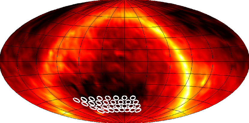
Figure 4: Locations of the DASI CMB fields, plotted over the IRAS $100~{}$micron map, in equatorial coordinates. (Color map is logarithmic, spanning 4 decades of intensity.)

While the current state of our knowledge of all of these Galactic foregrounds implies that the CMB will dominate the anisotropy signal at the frequencies and angular scales to which DASI is sensitive (see, e.g., Tegmark et al. 2000, for a comprehensive review), we employ an additional check which is independent of the assumptions and scaling laws presented above. As discussed in Paper II, when extracting the CMB power spectrum from the visibility data, we project out foregrounds on the basis of their spatial template alone, with no assumptions about the intensity of the various components at centimeter wavelengths. These constraints restrict the contribution of any of these diffuse foregrounds to be less than $\sim 3\%$ of the CMB signal, assuming only that the 26–36 GHz counterparts to these foregrounds have the same spatial distribution as they do at frequencies where the foregrounds are dominant; it is assumed that each diffuse foreground can be described with a constant single spectral index in a given DASI field.

5.2 Discrete Sources

As expected for cm-wave, small angular scale experiments, point sources are the dominant astronomical foreground for DASI (see, e.g., Tegmark & Efstathiou 1996), and the dominant contributor to the measured anisotropy. The method described above for projecting out diffuse foregrounds can be applied to point sources as well, since they produce a unique spatial signature in the visibility data. To null the effect of point sources through this technique, we therefore require only the positions of the sources, not their fluxes.

Positions for the brightest point sources are determined from the DASI data themselves; the procedure for identifying bright point sources is described in detail in §9 below. Positions for point sources below the DASI detection threshold are determined from the PMN catalog (Wright et al. 1994); in all, we constrain every point source from the PMN survey whose 5 GHz flux density, when modulated by the DASI primary beam, exceeds 50 mJy.

For sources below the PMN flux cutoff, we require a statistical correction to the power spectrum. These corrections, given explicitly in Paper II, are determined by Monte Carlo simulation of a point source population with $dN/dS$ given by the PMN catalog, and whose spectral index distribution is determined by observation of a complete sample of PMN sources with the OVRO 40-meter telescope at 26–36 GHz (paper in preparation).

5.3 Ground Contamination

Astronomical foregrounds aside, the presence of ground contamination at a level much greater than the expected cosmological signal places the most stringent constraint on our observing strategy. Although DASI was intended to operate with a ground shield, the panels could not be installed until the 2000–2001 austral summer and were not in place while the data described here were collected.

The signature of the ground is visible even in short integrations; as fields are tracked over the full azimuth range, excluding the MAPO building, variations as large as $7\,\sigma$ above the expected thermal noise ($\sigma\sim 4$ Jy) can be seen in 5-minute integrations, while directly over the roof of MAPO, 20-$\sigma$ signals are seen on a few of the shortest baselines. However, these fluctuations are strongly dependent on baseline length, falling sharply with increasing $(u,v)$ radius; on the longest baselines, the raw visibilities are consistent with thermal noise at all frequencies, even when observing directly over the MAPO building.

Although the ground shows a strong azimuthal dependence, repeated 24-hr tracks demonstrate that the signals are quite stable over time. When data taken as much as five days apart are differenced, the residuals are consistent with the thermal noise, even on the shortest baselines, and over the full azimuth range, including directions towards MAPO and other station buildings.

6 Observations

6.1 Field Selection

Because the ground signal exhibits long-term stability, our strategy was to observe independent fields over a narrow azimuth range on timescales short enough that the ground could be expected to remain constant. Observations were divided among groups of 8 fields separated by 1 h of RA, each group at a constant elevation. Each field in a group was observed over a fixed 1-hr azimuth range; over the course of 8 hours, these observations yield 8 samples of the CMB sky, and 8 independent samples of the same ground, allowing a constraint on the common mode (and reducing the effective number of degrees of freedom available for constraining the CMB power spectrum). Observations were timed so that data from each field sampled precisely the same ground. Azimuth ranges were selected which avoided lines of sight passing over any of the South Pole station or science buildings, or the communications antenna field.

Four such rows of 8 fields, referred to as the A–D rows, were arranged on a hexagonal grid (to facilitate eventual mosaicing of the fields), spaced by 1 h in RA and $6\arcdeg$ in declination. The grid of fields was positioned at high elevation ($\geq 49\arcdeg$), to further reduce the signal from the ground. Besides permitting a constraint on ground contamination, as discussed above, the spacing of 1 h in RA results in negligible inter-field correlations, greatly simplifying the analysis described in Paper II. Declinations and right ascensions of the first field in each row are given in Table 2.

TABLE 2
CMB Field Row Positions
Row	RA (J2000)	Dec (J2000)	Days Observed
A	$22\,\,00\,\,00$	$-61\,\,00\,\,00$	14
B	$21\,\,30\,\,00$	$-67\,\,00\,\,00$	24
C	$22\,\,30\,\,00$	$-55\,\,00\,\,00$	28
D	$23\,\,00\,\,00$	$-49\,\,00\,\,00$	31

6.2 Observing Schedule

As described above, in each 24-hr period, we obtained a total of 16 hours of integration on 8 CMB fields: 8 hours over each of two azimuth ranges. The remainder of a 24-hr period was divided among various calibration tasks. Every 8-hr period was bracketed by 1.5-hr scans on a calibrator source, as discussed in the next section, and these 11-hr periods were in turn bracketed by skydips, yielding two independent measures of the atmospheric opacity daily. These data are described in §4. Finally, at the beginning and end of every 24-hr period, the noise source was used to calibrate the complex correlator, as described in the next section.

7 Calibration

Several kinds of calibrations are performed for each of DASI’s 78 baselines, in each of the 10 bands: 1) calibration of the complex multipliers to correct for non-orthonormality of the real and imaginary visibility response, 2) absolute calibration of the flux scale for each baseline, which is transferred to a celestial source and 3) regular observations of celestial calibrators, to refer visibility amplitudes to the absolute flux scale and visibility phases to a phase center.

The second and third of these calibration tasks are described in separate sections below. The first, the calibration of the complex multipliers, was accomplished by injection of a strong signal from the correlated noise source. This calibration was performed at the beginning and end of every 24-hr period, although for $95\%$ of all baselines, the rms variation of the relative gain and phase offset between real and imaginary multipliers were less than $2\%$ and $1\fdg 2$, respectively, over 97 days.

7.1 Absolute Calibration

The relative scarcity of sources whose flux densities are known at high frequencies makes absolute calibration of any microwave experiment a challenging proposition, as does the generic steepness of most radio source spectra. Additionally, of the sources which are well studied, few are accessible from the South Pole. Planets never rise more than $\sim 23\fdg 5$ above the horizon, and the best studied of these, Jupiter and Mars, were either very low or below the horizon throughout the 2000 observing season. Moreover, with DASI’s 20-cm apertures, beam dilution makes it inherently difficult to detect all but the brightest point sources; with a gain of approximately $10~{}{\rm\mu K/Jy}$, to achieve a S/N $\sim 1$ per visibility on a 1 Jy source requires about an hour of observation.

Consequently, the absolute calibration of DASI is based on measurements of beam-filling external thermal loads of measured temperature. The noise source power level (which is separately monitored for drift) was calibrated for each receiver from these measurements, and a calibration of correlated noise source power was derived for each baseline. This calibration was immediately transferred from the noise source to a celestial source.

For the transfer observations, the source was tracked for 3 hours at each of six faceplate rotations, separated by $60\arcdeg$, with a reference field observed for ground subtraction. Due to the three-fold symmetry of the antenna locations, this procedure yielded six independent measurements of each $(u,v)$ point from different baselines with different contributions from the ground. The source model was averaged over these observations to reduce any residual systematics, resulting in a determination of the flux for each baseline with a statistical uncertainty of $<2\%$.

The load measurement and transfer procedure was conducted once during the austral summer of 2000 and again in the summer of 2001. The calibration of 2001, on which the absolute scale of the DASI observations is based, was transferred directly to PKS J0859-4731. The 2000 calibration was transferred without ground subtraction to the Carina Nebula and later to PKS J0859-4731 through interlaced observations of the two sources. We estimate the statistical uncertainty on the overall flux scale resulting from the load measurement procedure and transfer observations to be $<1\%$, averaged over baselines. Consistent with this estimate, the average ratio of fluxes derived from the independent calibrations of 2001 and 2000 is $0.997$. The systematic uncertainty common to these two calibrations, resulting mainly from uncertainty in the determination of antenna coupling to the loads and in the effective load temperatures, we estimate to be $3\%$, and is the dominant contribution to the total $3.5\%$ uncertainty in the overall flux scale.

7.2 Celestial Calibrators

As previously noted, each 8-hr period of CMB observations was bracketed by 1.5-hr scans of celestial calibrators to refer the visibility amplitudes to the absolute flux scale and to refer the phases to a common phase center. In addition, the correlated noise source was injected every hour to track short-term system stability. In practice, the instrumental phase and amplitude response were quite stable; over 97 days of observation, the phases showed a typical rms variation of less than $15\arcdeg$.

For the fields referred to as the A row in Table 2, the amplitude calibrator used was the Carina Nebula, a well-known Galactic HII complex. The Carina Nebula’s free-free spectrum makes it a good high frequency calibrator; the source is bright enough that its flux can be measured to a few percent on most baselines in approximately 15 minutes. However, the source is dominated by an extended central region, with much weaker flux on smaller scales, necessitating significantly longer integrations on the longest baselines to achieve uniform accuracy.

These considerations led us to use PKS J0859-4731, a more compact Galactic HII region, as the flux calibrator for the B–D row observations. Although its integrated flux is lower than that of the Carina Nebula (see Leitch et al. 2000), the source is readily detectable, with nearly uniform flux ($\sim 150~{}{\rm Jy}$) out to the longest baselines; for $(u,v)$ radii $>80~{}\lambda$, the source is considerably stronger than Carina.

Although PKS J0859-4731 is partially resolved by the longest baselines, observations of the source while rotating the faceplate show that the rms phase variation with parallactic angle, averaged over all baselines, is less than $10\arcdeg$. These observations indicate that PKS J0859-4731 is sufficiently point-like (or at least radially symmetric) that the source can be used as a phase calibrator. Although PKS J0859-4731 is located in the Galactic plane, these observations also demonstrate that any contaminating flux is small.

Thus, for the B–D row data, each 1.5-hr scan was spent observing PKS J0859-4731, which was used as both amplitude and phase calibrator. For the A-row observations, this time was split between the Carina Nebula and the extragalactic source Centaurus A, which served as the phase calibrator. On all but the longest baselines of the A-row data, these observations yielded measurements of both phase and amplitude to better than $2\%$.

8 Data Reduction

The data presented in this paper (and analyzed in Papers II and III), comprise 97 days of observations obtained during 05 May–07 November 2000, divided among 32 fields, as described in §6.1. These data represent an observing efficiency of approximately $85\%$ of the time devoted exclusively to CMB observations; the remainder of the time was lost to hardware maintenance and reliability. Because our ability to constrain the ground depends critically on uniform sampling of a fixed azimuth range for each of 8 fields, as described in §5.3, a draconian pre-edit is applied to the CMB data – the loss of all data for a single field for any reason results in the rejection of the entire 8-hour period for that baseline and correlator band.

Visibilities are accumulated from each correlator in 8.4-s integrations, along with monitor data from the telescope drive systems and receivers. Prior to combination for input to the power spectrum analysis described in Paper II, various edits are applied to these data, falling into three general categories: cuts on monitor data, cuts derived from the visibility data themselves, and calibration edits.

In the first category, data are rejected when a receiver is not operating, when a receiver LO loses lock, or when either the 10 or 50 K cryogenic receiver stages shows a gross warming trend; these cuts typically reject $\sim 5\%$ of the data. Next, data are edited on the quadrature errors in the complex multipliers, determined twice daily by injection of a broad-band noise source. Baselines for which the relative gain between the real and imaginary multipliers falls outside the range $0.9\pm 0.3$ (deviation of the mean value from 1 reflects the signal path asymmetry introduced by the hybrid splitters), or for which the phase offset falls outside the range $0\arcdeg\pm 20\arcdeg$, are rejected. These ranges are determined from the empirical distribution of quadrature errors and reflect the values at which the distributions become significantly non-Gaussian; these data are interpreted as evidence for microstrip termination errors or malfunctioning multiplier chips and showed little variation throughout the 2000 season. When the raw visibilities are calibrated for these offsets, data are rejected if the bracketing values differ by more than $10\%$. Cuts on the quadrature errors collectively reject $\sim 11\%$ of the data.

The closest approach of the moon to the DASI fields during their observation is $36^{\circ}$. Fringing from the moon is evident on the shortest baselines, and for $(u,v)$ radii $<40\,\lambda$, we reject all data when the moon is above the horizon. The D-row observations were made from 11 September–11 October, bracketing the sunrise, with an additional week obtained in early November; data for the D-row fields are also excluded for $(u,v)$ radii $<40\,\lambda$ when the sun is above the horizon.

In the second category of edits, the raw visibilities are combined into 1-hr bins, and the baseline-baseline correlation matrix is computed separately for each correlator. Large off-diagonal elements of the correlation matrix are interpreted as evidence for contamination by atmospheric fluctuations. By comparison of data for the same field from different azimuth ranges on the same day, or from different days, we find that the precise threshold of the correlation cut does not strongly affect data consistency, and we reject an 8-hr observation for which any off-diagonal element exceeds $\pm 0.36$, affecting $5\%$ of the data.

In the last category, data are edited on the quality of the associated observations of celestial phase and amplitude calibrators. Data are rejected when the bracketing calibrator amplitudes vary by $>10\%$, or when the bracketing phases change by $>30\arcdeg$. Data are also rejected when previous edits have reduced the sensitivity on a calibrator scan by $>\sqrt{2}$, resulting in a statistical error of $>3\%$. On average, these cuts reject $\sim 20\%$ of the data. Overall, the combined edits from all categories reject a total of 40% of the data.

For input to the power spectrum analysis described in Paper II, the edited and calibrated data are combined into 1-hr integrations, yielding a maximum of 1560 visibilities per field (78 complex baselines$\times$10 correlator channels) for each observation.

9 Point Sources

The brightest point sources in our fields are obvious in the synthesized maps (see Figure 2), even without ground subtraction. However, as discussed in Paper II, and in §5 above, to extract the CMB power spectrum from the visibility data, we employ a method capable of projecting out point sources on the basis of their positions alone. As described in Paper II, we construct the list of point sources to null using a combination of source positions derived from the DASI data, as well as positions of sources in the PMN southern catalog. Here we describe the procedure used to find sources in the DASI data.

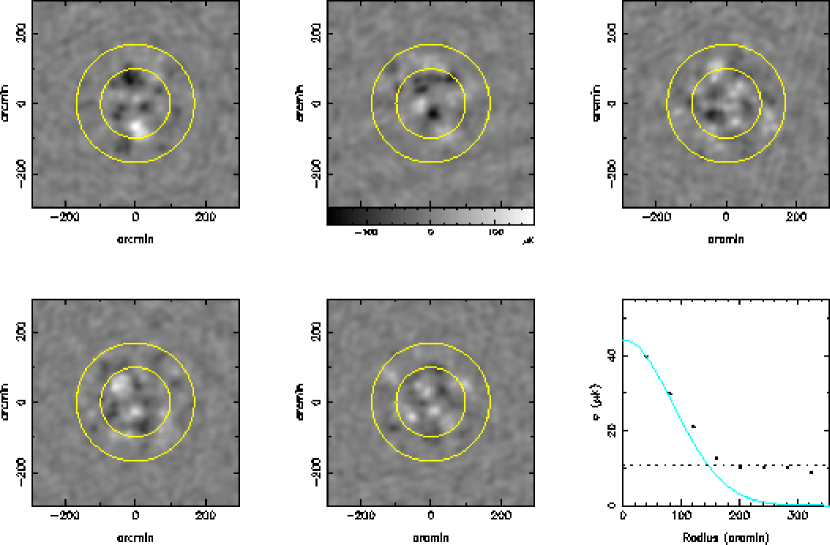
Figure 5: Images of five DASI CMB fields. The two concentric circles represent the $-3$ dB and $-10$ dB taper of the beam, respectively. The lower right panel shows the rms pixel values for field 5 (lower middle panel) as a function of radius (black points), the primary beam taper normalized to the first rms pixel value (solid line), and the theoretical rms image noise, determined from the scatter in 8.4-s visibility data (dashed line).

For each set of fields, images are made from ground-subtracted visibilities using the DIFMAP imaging package (Shepherd, Pearson, & Taylor 1994). When making the images, baselines $<64~{}\lambda$ are excluded; this cut removes the bulk of the CMB power in the data, significantly increasing the S/N for point source detection. The maps are then divided into annular bins around the field center; the pixel rms in each bin, averaged over 8 fields, is fit to a noise model, consisting of a signal with the shape of the primary beam, added to a flat detector noise floor (as in the bottom right panel of Figure 5). Each image is then divided by the fitted noise model to produce an effective S/N map. The highest peaks, multiplied by a copy of the synthesized beam, are then iteratively subtracted from the image until no peaks $>4.5$ remain; we estimate that in the absence of point sources, 0.03 peaks above this threshold should occur in each set of 8 fields.

Using this technique, we can detect a 40 mJy source at beam center with $>4.5$-$\sigma$ significance. In the 32 DASI fields, we find 28 sources, whose estimated $S_{31}$ fluxes range from 80 mJy to 7 Jy. Correlating these locations with the PMN catalog, we find $S_{5}>100$ mJy counterparts for them all, with probabilities for accidental association $\lesssim 0.01$. Positional errors are typically several arcminutes. However, note that the PMN survey will resolve some of the closest sources, yielding positions which may differ from the effective position as seen by DASI. This limits the determination of our absolute pointing error, but we estimate it to be better than $2^{\prime}$.

Fitting the position of the very brightest sources for each day of data over the observations of a given set of fields shows that pointing drift over $\sim 30$ days is $<1^{\prime}$. Servo tracking jitter is $\ll 1^{\prime}$ and the fact that point sources appear in the maps with exactly the shape of the synthesized beam confirms this.

10 Results

Although Fourier plane visibilities are the natural data product of an interferometer, image-plane analysis provides a valuable consistency check on the data quality. Shown in Figure 5 are a subset of the DASI fields, after point source removal and ground subtraction. In these images, point sources identified in the DASI data were removed by subtraction of a delta function model from the visibilities, while ground contamination has been removed by subtraction of a mean visibility, averaged over 8 fields, from each of the 1-hr field integrations. Artifacts of the $(u,v)$ sampling have been reduced in these maps by a variant of the CLEAN algorithm (Högbom 1974), restricted to the $-10~{}{\rm dB}$ contour of the primary beam, similar to the procedure described in §9 for finding point sources.

For an interferometer, each visibility is convolved with the autocorrelation of the antenna aperture; in the image plane, this translates into an enveloping of the image by the primary beam. Here the images have been deliberately extended to radii well beyond the central beam area, so that detector noise should dominate near the edges. As can be seen qualitatively in Figure 5, after a simplistic removal of the ground and point source signals, every field shows residual structure in the central region of the beam; as demonstrated in the lower right panel, the rms in radial bins follows the beam profile, tapering to the theoretical noise floor, typically $10~{}{\rm\mu K}$ (at $\sim 20^{\prime}$ resolution), far from the beam center.

Images of the same fields observed at different epochs show repeatable structure, and when images are constructed from visibilities divided into two frequency ranges, the ratio of pixel values is consistent with a thermal spectrum (see Leitch et al. 2000); rigorous, Fourier-plane analogues of these tests are described in Paper II.

The entire complement of 32 DASI fields is shown in Figure 6, after ground and point source removal. Here we show only the central FWHM of each field, corrected for the primary beam taper at the center of the band. Although the S/N is high enough in all these maps that the apparent structure is real, note that the sensitivity is not uniform across the images, but decreases by a factor of 2 at the edges due to the primary beam correction.

We stress that these images are for presentation purposes only; no images are used in our power spectrum analysis, nor are point sources or ground ever subtracted from the visibility data; these foregrounds are modeled in a self-consistent way as part of the constraint matrix formalism presented in Paper II.

11 Conclusions

We have described the instrumentation, observations and first year data from DASI, a novel interferometric experiment to measure anisotropy in the CMB. During its first season of operation, the instrument functioned extremely well, producing 97 days of high-quality data on 32 CMB fields, for an average of 24 hours of integration per field, and achieving close to the theoretical noise limits.

With these data, we are able to image $\sim 400$ square degrees of sky to a typical rms sensitivity of $10~{}\mu$K (at $\sim 20^{\prime}$ resolution); we detect structure in the CMB with high S/N in every field. Although the ground has proven to be our largest contaminant, the slowly varying character of this foreground and careful experiment design enables us reliably to recover the CMB component, even in the presence of near-field signals many times the amplitude of the intrinsic fluctuations. As detailed in Paper II and Paper III, these data yield a sensitive new measurement of the CMB power spectrum and provide important constraints on cosmological parameters.

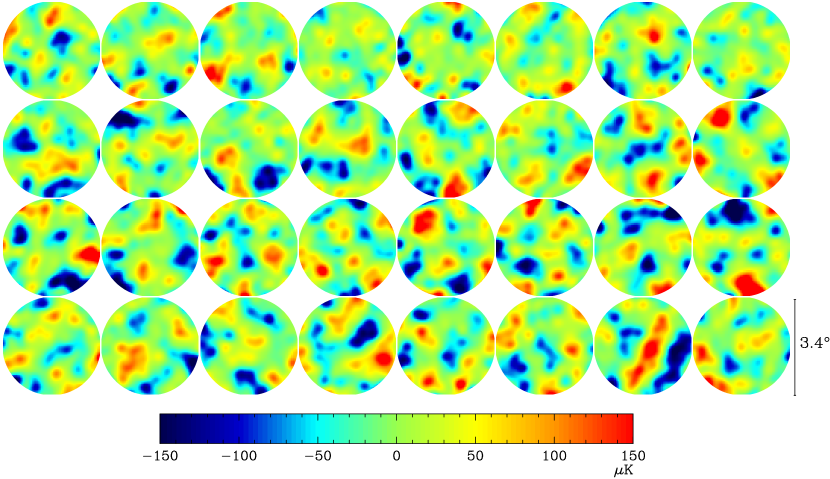
Figure 6: Images of the 32 DASI fields, at $20^{\prime}$ resolution. Shown are CLEANed maps of the central $3\fdg 4$ FWHM of each primary beam, corrected for the beam taper. Typical rms noise in a $20^{\prime}$ beam is $10\,{\rm\mu K}$ at map center; note however, that because these images have been divided by the primary beam, the effective noise increases by a factor of 2 at the map edges. Rows are in order of decreasing elevation: B, A, C, D from bottom to top, with RA increasing to the left.