On the time variability of $\gamma$-ray sources: A numerical analysis of variability indices

We present a Monte Carlo analysis of the recently introduced variability indices $\tau$ (Tompkins 1999) and $I$ (Zhang et al. 2000 & Torres et al. 2001) for $\gamma$-ray sources. We explore different variability criteria and prove that these two indices, despite the very different approaches used to compute them, are statistically correlated (5 to 7$\sigma$). This conclusion is maintained also for the subset of AGNs and high latitude ($|b|>10$ deg) sources, whereas the correlation is lowered for the low latitude ones, where the influence of the diffuse galactic emission background is strong. END

gamma-rays: observations – variability END

1 Introduction

The study of the time variability of $\gamma$-ray sources, particularly using the Third EGRET Catalog (Hartman 1999), is currently a very active topic of research. The Third EGRET Catalog includes observations carried out between April 22, 1991 and October 3, 1995, and lists 271 point sources. About two thirds of them have no conclusive counterparts at lower frequencies. Even worse, 40 of them do not show any positional coincidence (within the 95% EGRET contour) with possible $\gamma$-ray emitting objects known in our galaxy (Romero et al. 1999).

In order to understand the origin of all these unidentified detections, their variability status is of fundamental importance. Several known models for $\gamma$-ray sources in our galaxy would produce non-variable sources during the timescale of observations. That is the case of pulsars (Thompson 2001) or supernova remnants in interaction with molecular clouds (Esposito et al. 1996, Combi et al. 1998, 2001). Alternatively, if some of the sources are produced by isolated magnetized black holes (Punsly et al. 2000), microquasars (Paredes et al. 2000), or by stellar winds of early type stars (Benaglia et al. 2001) one would expect high levels of flux variability.

Looking at the flux evolution through the different viewing periods is obviously a first indication of the variability status of any given source (see for instance Tavani et al. 1997). However, fluxes are usually the result of only a handful of incoming photons. A safer way of quantifying the flux evolution should be devised before obtaining significant results.

2 Variability indices

2.1 The $V$-index for $\gamma$-ray variability

Three variability indices have been introduced in the literature so far. The first of them, dubbed $V$, was presented by MacLauglin et al. (1996), who computed it for the sources contained in the Second EGRET Catalog. This method was later used, also, for a short timescale study by Wallace et al. (2000). The basic idea behind $V$ is to find $\chi^{2}$ for the measured fluxes, and to compute $V=-\log Q$, where $Q$ is the probability of obtaining such a $\chi^{2}$ if the source were constant. Several critiques have been mentioned concerning this classification, among them, that the scheme gets complicated when the fluxes are just upper limit detections. It can be shown that sources which have upper limits included in the analysis will have a lower $V$ than that implied by the data (Tompkins 1999). In addition, a source can have a large $V$ because of intrinsic reasons –the case we would be interested in–, or because of small error bars on the flux measurements. Similarly, a small value of $V$ can imply a constant flux or big error bars. Each value of $V$ is obtained disregarding those of a control population. Then, we can have pulsars with very high values of $V$, or observed AGNs with very low ones. The use of $V$ to classify the variability of $\gamma$-ray sources seems not to be very confident.

2.2 The $\tau$-index for $\gamma$-ray variability

Tompkins (1999) introduced a new variability criterion which takes into account not only published EGRET data, contained in the point source 3EG Catalog, but also unpublished information. In order to decide the variability index for a given source he used also the 145 marginal sources that were detected but not included in the final official list, and, all at a time, the detections within 25 deg of the source of interest. The maximum likelihood set of source fluxes was then re-computed. From these fluxes, a new statistics measuring the variability was defined as $\tau=\sigma/\mu$, where $\sigma$ is the standard deviation of the fluxes and $\mu$ their average value. The strength of this approach lies in that it takes into account some possible fluctuations from the background and from neighboring sources, careful sensitivity corrections throughout EGRET lifetime, and others systematic errors related either with the equipment itself or with the processing of the information, in a similar way to that used in the construction of the 3EG (Hartman et al. 1999, Tompkins 1999). Details are to be given in Tompkins et al. (2001). The final result of Tompkins’ analysis is a table listing the name of the EGRET source and three values for $\tau$: a mean, a lower, and an upper limit (68% error bars).

2.3 The $I$-index for $\gamma$-ray variability

This index was previously used in blazar variability analysis (Romero et al. 1994) and applied to some of the 3EG sources by Zhang et al. (2000) and Torres et al. (2001). The basic idea is to do a direct comparison of the flux variation of any given source with that shown by pulsars, which is considered spurious. Then, the $I$-index establishes how variable a source is with respect to the pulsar population. Contrary to Tompkins’ index, the $I$-scheme uses only the publicly available data of the 3EG Catalog.

The $I$ index is defined as follows. Firstly, a mean weighted value for the EGRET flux is computed:

$$\left<F\right>=\left[\sum_{i=1}^{N_{{\rm vp}}}\frac{F(i)}{\epsilon(i)^{2}}\right]\times\left[\sum_{i=1}^{N_{{\rm vp}}}\frac{1}{\epsilon(i)^{2}}\right]^{-1}.$$ (1)

$N_{{\rm vp}}$ is the number of single viewing periods for each $\gamma$-ray source, $F(i)$ is the observed flux in the $i^{{\rm th}}$-period, whereas $\epsilon(i)$ is the corresponding error in the observed flux. These data are taken directly from the 3EG catalog. For those observations in which the significance ($\sqrt{TS}$ in the EGRET catalog) is greater than 2$\sigma$, we took the error as $\epsilon(i)=F(i)/\sqrt{TS}$. For those observations which are in fact upper bounds on the flux, it is assumed that both $F(i)$ and $\epsilon(i)$ are half the value of the upper bound. Then, the fluctuation index $\mu$ is defined as:

$$\mu=100\times\sigma_{{\rm sd}}\times\left<F\right>^{-1}.$$ (2)

In this expression, $\sigma_{{\rm sd}}$ is the standard deviation of the flux measurements, taking into account the previous considerations.

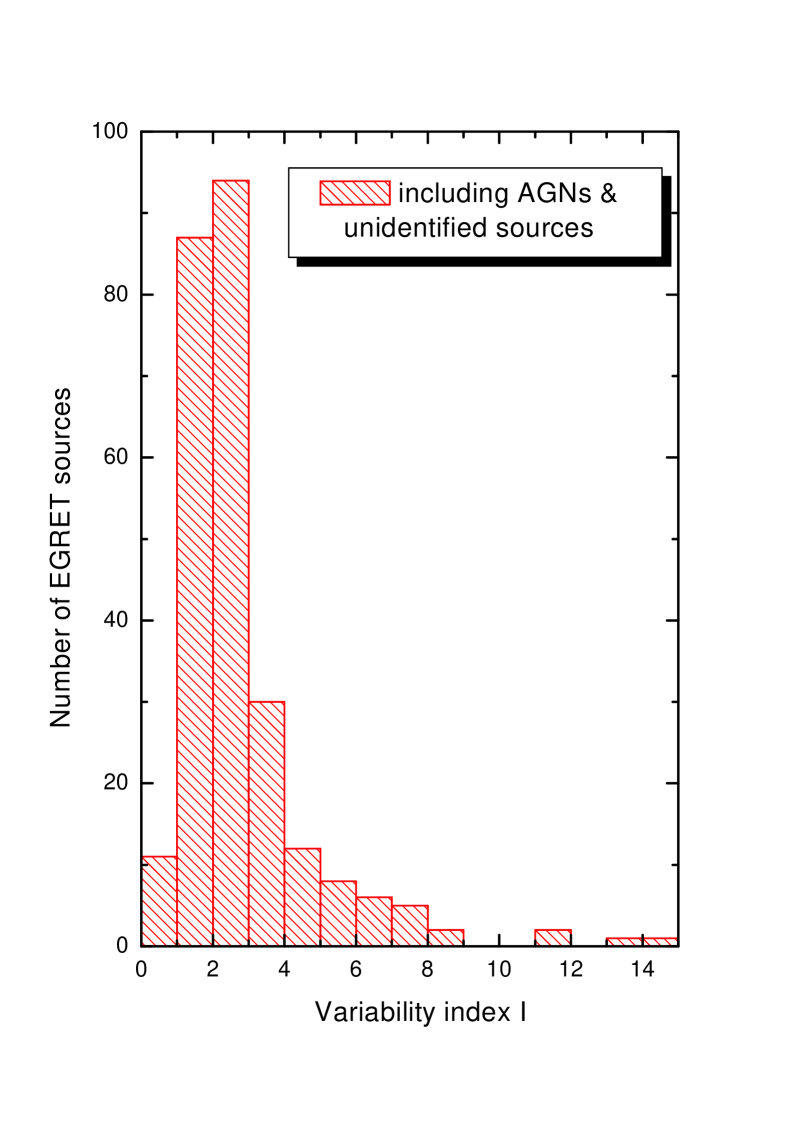
Figure 1: Variability index distribution for 258 $\gamma$-ray sources in the Third EGRET Catalog, excluding pulsars and six artifacts related with Vela.

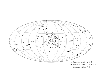
Figure 2: Sky variability distribution, under the $I$-scheme, of 258 $\gamma$-ray sources in the Third EGRET Catalog. Up triangles stand for (25) variable sources, circles for (157) dubious, and a down triangles for (76) non-variable. Thresholds are as in Table 1.

This fluctuation index is also computed for the confirmed $\gamma$-ray pulsars in the 3EG catalog, assuming the physical criterion that pulsars are –i.e. by definition– non-variable $\gamma$-ray sources. Then, any non-null $\mu$-value for pulsars is attributed to experimental uncertainty. Finally, the averaged statistical index of variability, $I$, is given by

$$I=\frac{\mu_{{\rm source}}}{<\mu>_{{\rm pulsars}}}=\frac{\mu_{{\rm source}}}{26.9}.$$ (3)

In Fig. 1 we show the histogram of $I$ for 258 $\gamma$-ray sources in the 3EG Catalog, and in Fig. 2, the sky distribution.

3 From variability indices to variability criteria

3.1 Plausible criteria for $\tau$

The index $\tau$ moves from 0 upwards, and it is considered infinite when it is greater than 10 000. As can be seen from Tompkins (1999), the thresholds for variability are diffuse. To have an idea of what a variable source is under the $\tau$-scheme, Tompkins has separated the $\gamma$-ray sources into different classes: pulsars, unidentified, AGNs, and sources spatially coincident with SNRs. He found that $\tau$ can clearly distinguish between pulsars, whose mean $\tau$-value is 0.1, having the highest upper limit equal to 0.27, and AGNs, whose mean is 0.9. The unidentified sources have $\tau$-values pertaining to both categories. Many sources clearly have a dubious classification; for instance, 3EG J1339-1419 has a mean $\tau$-value equal to 0.68, but their lower and upper limits are, respectively, 0.17 and 1.70. Then, within the 68% error bars on $\tau$, this source can be as variable as an AGN, or as non-variable as a pulsar. This is an uncomfortably common situation for many sources.

However, if the lower limit on $\tau$ is greater than, say, 1.0, the source is very likely variable. If the upper limit on $\tau$ is, on the contrary, compatible with the $\tau$-values for pulsars, we would classify it as non-variable. This encompasses the spirit of Tompkins’ (1999) classification of the most likely variable and the most likely non-variable sources. The question is then what the thresholds should be. We have seen that pulsars are consistent with values of $\tau$ up to 0.27. The deviation for the mean value of pulsars is $\sim 0.1$. Then, it appears safe to consider that a source will be likely variable –under the $\tau$ scheme– when the lower limit on $\tau$ is at least 0.6, $3\sigma$ above the mean value of the $\tau$ upper limit for pulsars. Equivalently, a source will be considered non-variable when the upper limit for $\tau$ is below that threshold. Sources not fulfilling either classification should be considered as dubious.

We can modify these thresholds in a number of ways, but we want pulsars to represent a non-variable population, and AGNs to be, on average, a variable one. But even fulfilling these constraints, we could better use a 2 or 4$\sigma$ level as a safe assumption, or pretend to artificially move the threshold to $\sim 0.3$, just above the highest possible level for pulsar variability. We have explored these assumptions case by case, by means of a computer code described below, and although we found no statistically strong variations in the final classification, we did find that a threshold of 0.5–0.6 is the safer. Known variable sources end up classified as variable, known or expected non-variable ones also get their right status.

3.2 Plausible criteria for $I$

One possibility for defining a variability criterion for $I$ is also to consider the error bars for each source:

$$\delta I=\frac{\mu}{<\mu>_{{\rm pulsars}}^{2}}\delta<\mu>_{{\rm pulsars}}\sim 0.5\;I.$$ (4)

Here $\delta<\mu>_{{\rm pulsars}}$ is the deviation from the $<\mu>_{{\rm pulsars}}$-value. Then, we have just propagated through $I$ the error in defining the mean value of the fluctuation index for pulsars. We can then define variable sources as those fulfilling the constraint

$$I-\delta I>I_{p}+3\sigma,$$ (5)

and non-variable sources as those having

$$I+\delta I<I_{p}+3\sigma.$$ (6)

Here, $I_{p}=1.0$, is the mean value of $I$ for pulsars, and $\sigma=0.5$, is the deviation in the pulsar $I$-values. Again, sources not fulfilling neither classification are to be considered dubious. Then, rephrasing the previous two equations we get variable sources when $I>5.0$, non-variable sources when $I<1.7$, and dubious cases for $I$-values in between. These are very conservative and restrictive constraints, and have close analogy with the proposed ones for the $\tau$-index. Particularly, notice that if $I>5.0$ is the threshold for a variable source, then we are asking for the value of $I$ to be 8$\sigma=8\times 0.5$ times above that of pulsars. Similarly, for a source to classify as non-variable, its $I$-index should depart from that of the pulsars in less than 1.4$\sigma$.

This may sound excessive. In addition, why does $3\sigma$ appear in Eqs. (5) and (6), not 2 or 4? We can as well use the mean value of $I$ in a direct way, so defining a more straightforward scale. We can assume a source to be non-variable if its $I$-value is less than 1.5 (1$\sigma=1+0.5$ above the pulsars), dubious for $1.5<I<3.5$, and variable for $I>3.5$, 5$\sigma$ above the mean $I$-index for pulsars. That would be, although less restrictive, as good a criterion as the previous one. Changing the criteria will obviously change the variability status of those sources with values of $\tau$ and $I$ near the boundaries. We then need to explore all these possibilities in a systematic way before extracting significant conclusions.

4 Results of the numerical analysis

We have written a numerical code that classifies the source variability, given any chosen criteria, both in the $I$ and the $\tau$ scheme. In the Internet address provided below we present complete tables quoting together the $I$ and $\tau$ indices for each of the sources in the 3EG Catalog. We present in Table 1 the results for the classification using the above explained criteria: $\tau$-threshold equal to 0.6, and $I$-thresholds equal to 1.7 and 5.0, respectively. There are 148 detections out of 258 –five pulsars and six artifacts related with Vela were excluded– (57% of the sources) which classify within the same groups both for $I$ and $\tau$. Can this percentage be obtained randomly?

Table 1: Classification of all 258 sources (excluding pulsars and six artifacts related with Vela) reported in the Third EGRET Catalog. Pulsars are non-variable sources in both schemes. The $\tau$-threshold is equal to 0.6, and the $I$-thresholds are equal to 1.7 and 5.0, respectively. The row dubbed ‘Same class’ shows the number of sources that classify within the same group in both schemes.

Scheme	variable	dubious	non-variable
$I$	25	157	76
$\tau$	55	139	64
Same class	17	95	36

We have simulated thousands of sets of 258 sources and assigned to each of them a random variability index $I$. We preserved the histogram for $I$, i.e. the number of variable, dubious, and non-variable detections is the same in each of the simulated sets, but they are assigned to randomly chosen sources. Should we not preserve the histogram for $I$, we would admit, for instance, a random case in which all sources are variable, another in which all are non-variable, etc. This would diminish the random probability of obtaining the real result in an inappropriate way. What we want to test is the actual classification which associates a particular source with a particular value of $I$; this is why, while maintaining the $I$ distribution, we shuffle the associations.

Not only the percentages of equal classification are important in order to decide if the two schemes are statistically correlated, but also the expected random result. For instance, if the thresholds are chosen such that all sources are non-variable in both schemes, then the percentage of equal classification would be 100%. But so would be the random percentage for each of the simulated sets, and then there would be no correlation at all.

We found that the expected random result is 104.8$\pm$6.3, i.e. 7$\sigma$ below the real result, implying for it a Poisson probability equal to 8$\times 10^{-6}$. We have also used several alternative plausible thresholds both for $I$ and $\tau$, for instance, $\tau$-thresholds equal to 0.8, 0.5, and 0.35, with $I$-thresholds equal to 5.0/2.0, 5.0/1.7, and 3.5/1.5. In all cases, we obtain a percentage of equal classification above 50%, the worst random result (obtained for $\tau$-thresholds equal to 0.35 and $I$-thresholds equal to 3.5/1.5) being still 5$\sigma$ lower than the real one. Thus, disregarding the fine grain of the variability criteria, the two schemes are statistically correlated. We have also explored what happens if we do not consider those sources having an average recomputed flux equal to 0.00 within the $\tau$-scheme (Tompkins 1999). Doing the simulations excluding these sources produces an even more correlated result.

In Table 2 we show the results for the 67 AGNs. 44 (65%) of them have the same classification within both schemes, while we would expect only 31$\pm$3.0 as a result of chance, 5$\sigma$ lower than the real result. Again, changing the criteria does not significantly alter the results (and in most cases actually improves them).

Table 2: Classification of confirmed AGNs reported in the Third EGRET Catalog. Thresholds are as in Table 1.

Scheme	variable	dubious	non-variable
$I$	10	42	15
$\tau$	15	40	12
Same class	7	30	7

Table 3 shows the results both for high ($|b|>10$ deg) and low latitude sources. For the former, the random result is $4\sigma$ below the real one. Changing the criteria to all other plausible ones we have discussed above enhances the correlation. For the low latitude sources, the result is $3\sigma$ away from the real one. Here, changing the criteria to any other of the plausible ones we mentioned does not generally improve the correlation. The decrease in statistical correlation between $I$ and $\tau$ at low galactic latitudes, for the less restrictive criteria, could be reflecting the uncertainties in the subtraction of the diffuse background emission of the galaxy (Hunter et al. 1997, Strong et al. 2000).

Table 3: Classification of unidentified sources reported in the Third EGRET Catalog. The upper panel refers to high latitude sources and the lower one to low latitude detections. Thresholds are as in Table 1.

Scheme	variable	dubious	non-variable
$I$	12	74	34
$\tau$	34	61	25
Same class	8	39	15
$I$	3	41	27
$\tau$	6	38	27
Same class	2	26	14

5 Discussion and concluding remarks

The status of a particular source can vary from one scheme to the other. Then, the joint use of $I$ and $\tau$ can provide a better idea of the variability status of any given source. Particular classifications may disagree as a result of completely different techniques for computing the variability indices. Note that the dubious classification of any $\tau$ plausible criterion is applied upon sources we know nothing about. This is not the case for $I$, since it always provides a scale relative to the mean of the pulsar fluctuation indices. Then, it rests on our own judgement to decide the weight we shall give to a result like $I=3.0$, but it undoubtedly says that the flux evolution is three times more variable than the mean flux evolution for pulsars. We mention that in order to get more reliable results under the $I$-scheme at low latitudes it seems safer to consider the most restrictive cutoffs.

It has been noted (R. Hartman, private communication, 2001) that the weighting used for the definition of $I$ (as done in Zhang et al. (2000) and Torres et al. (2001)): an inverse square for the errors in the fluxes, could provide values of $<F>$ unrealistically high. The combined use of unweighted averages, and the definitions $F\sim\sqrt{TS}/(2+\sqrt{TS})$ and $err(F)\sim 1/(2+\sqrt{TS})$ for the the exposures showing only upper limits, could even improve the correlation with Tompkins’ index. But this would be another index for quantifying variability, not yet used in the literature.

- [1] Benaglia P., Romero G.E., Stevens I. and Torres D.F. 2001, A&A 366, 605
- [2] Combi J.A., Romero G.E., Benaglia P. 1998, A&A 333, L91
- [3] Combi J.A., Romero G.E., Benaglia P., Jonas J. 2001, A&A 366, 1047
- [4] Cusumano G., Maccarone M.C., Nicastro L., Sacco B., Kaaret P. 2000, ApJ 528, L25
- [5] Esposito J.A., Hunter S.D., Kanbach G., Sreekumar P. 1996, ApJ 461, 820
- [6] Hartman R.C., Bertsch D.L., Bloom S.D., et al. 1999, ApJS 123, 79
- [7] Hunter S. D. et al. 1997, ApJ 481, 205
- [8] Kaspi V.M., Lackey J.R., Mattox J., Manchester R. N., Bailes M., Pace R. 2000, ApJ 528, 445
- [9] McLaughlin M.A., Mattox J.R., Cordes J.M., Thompson D.J. 1996, ApJ 473, 763
- [10] Paredes J. M., Marti J., Ribo M., Massi M. 2000, Science, 288, 2340
- [11] Punsly B., Romero G.E., Torres D.F., Combi J.A 2000, A&A, 364, 556
- [12] Romero G.E., Combi J.A., Colomb F.R. 1994, A&A 288, 731
- [13] Romero G.E., Benaglia P., Torres D.F. 1999 A&A 348, 868
- [14] Strong A. W., Moskalenko I. V., Reimer O. 2000, ApJ 537, 763
- [15] Tavani M., Mukherjee R., Mattox J.R., et al. 1997, ApJ 479, L109
- [16] Thompson D. J. 2001, astro-ph/0101039, Gamma Ray Pulsars: Observations. To appear in International Symposium on High-Energy Gamma-Ray Astronomy, Heidelberg, Germany.
- [17] Tompkins W. 1999, Ph.D. Thesis, Stanford University.
- [18] Tompkins W. et al. 2001, In preparation.
- [19] Torres, D. F., Romero G. E., Combi J., Benaglia P., Punsly B., Andernach H. 2001, A&A, 370, 468
- [20] Wallace P.M., Griffis N.J., Bertsch D.L., et al. 2000, ApJ 540, 184
- [21] Zhang L., Zhang Y.J., Cheng K.S. 2000, A&A, 357, 957