Study of star formation in RCW 106 using far infrared observations

Abstract

High resolution far-infrared observations of a large area of the star forming complex RCW 106 obtained using the TIFR 1m balloon-borne telescope are presented. Intensity maps have been obtained simultaneously in two bands centred around 150 and 210 $\mu$m. Intensity maps have also been obtained at the four IRAS bands using HIRES processed IRAS data. From the 150 and 210 $\mu$m maps, reliable maps of dust temperature and optical depth have been generated. The star formation in this complex has occurred in five linear sub-clumps. Using the map at 210 $\mu$m, which has a spatial resolution superior to that of the IRAS at 100 $\mu$m, 23 sources have been identified. The spectral energy distribution (SED) and luminosity of these sources have been determined using the associations with the IRAS maps. Luminosity distribution of these sources has been obtained. Assuming these embedded sources to be ZAMS stars and using the mass-luminosity relation for these, the power law slope of the initial mass function is found to be $-1.73\pm 0.5$. This index for this very young complex is about the same as that for more evolved complexes and clusters. Radiation transfer calculations in spherically symmetric geometry have been undertaken to fit the SEDs of 13 sources with fluxes in both the TIFR and the IRAS bands. From this, the r^-2 density distribution in the envelopes is ruled out. Finally, a correlation is seen between the luminosity of embedded sources and the computed dust masses of the envelopes.

1 INTRODUCTION

Far-Infrared (FIR) observations provide an important tool to study formation of high mass stars, especially at a very early stage of their formation when they are deeply embedded in their parent clouds. The TIFR group has been active in observing in the FIR, especially at trans-IRAS wavelengths, using the TIFR 1m balloon-borne telescope (Ghosh et al. 1988; Ghosh et al. 1989a; Ghosh et al. 1989b; Ghosh et al. 1990; Ghosh et al. 2000; Verma et al. 1994; Mookerjea et al. 1999; Mookerjea et al. 2000). Taking advantage of our location, we have been mapping several star forming complexes in the southern hemisphere, not easily accessible from the higher latitudes of northern hemisphere. Balloon-borne telescope is also efficient in mapping a large area with moderate sensitivity. In this paper we describe our study of high mass star formation in RCW 106, a large southern star forming complex. This complex, harbouring a score or more of high mass stars, provides us an opportunity to study the mass function of stars at a very early stage and the physical conditions of their envelopes. This is aided by our simultaneous mapping at 150 and 210 $\mu$m with a high spatial resolution of $\sim 1\arcmin$ enabling us to resolve more sources than the IRAS at 100 $\mu$m.

RCW 106 is an optically visible H ii region in the southern Galactic plane. The distance of this H ii region is 3.6 kpc [Lockman 1979]. It was discovered by Rodgers, Campbell & Whiteoak (1960) while they were surveying the southern milky way in H$\alpha$ line emission. Radio continuum emission towards this region has been mapped by Shaver & Goss (1970a) and Goss & Shaver (1970) at 408 MHz and 5000 MHz. Interferometric observations of a part of the region are available at 1415 MHz (Retallack & Goss, 1980), 1420 MHz (Forster et al. 1987), 6.67 GHz and 8.64 GHz (Walsh et al. 1998). The associated molecular cloud was detected by Gillespie et al. (1977) during their observations of southern Galactic H ii regions in the J = 1–0 transition of CO. Similarly, interstellar molecules like OH [Caswell & Haynes 1975], H₂O [Kaufmann et al. 1977], NH₃ [Batchelor et al. 1977], CS [Gardner & Whiteoak 1978] and H₂CO [Gardner & Whiteoak 1984] were detected towards this region indicating extremely dense molecular material. Several maser sources in the lines of H₂O (Batchelor et al. 1980; Braz & Scalise 1982; Braz et al. 1989; Scalise, Rodriguez & Mendoza-Torres 1989), OH [Caswell, Haynes & Goss 1980] and methanol (Macleod & Gaylard 1992; Schutte et al. 1993; Caswell et al. 1995; van der Walt, Gaylard & Macleod 1995; van der Walt et al. 1996; Ellingsen et al. 1996; Macleod et al. 1998) have been detected towards this complex in independent surveys and observations towards selected IRAS sources. All these suggest ongoing high mass star formation in the region.

In the next section we describe the observations and details of the photometer employed. In Sec. 3 the intensity maps in the two bands and the derived maps of dust temperature and optical depth are presented. Intensity maps from HIRES processed IRAS observations are also presented in the four IRAS bands. Sources extracted from these maps and the spectral energy distribution (SED) derived from our and IRAS observations as well as the comparison of FIR sources with the radio continuum sources are also presented. Sec. 4 presents a discussion of the FIR luminosity distribution and the initial mass function (IMF) derived from this. Sec. 5 describes the physical properties of the envelopes of selected sources based on radiation transfer modelling. The results are summarised in the last section. More details of this study can be found in the PhD thesis of Karnik (Karnik 2000).

2 Observations

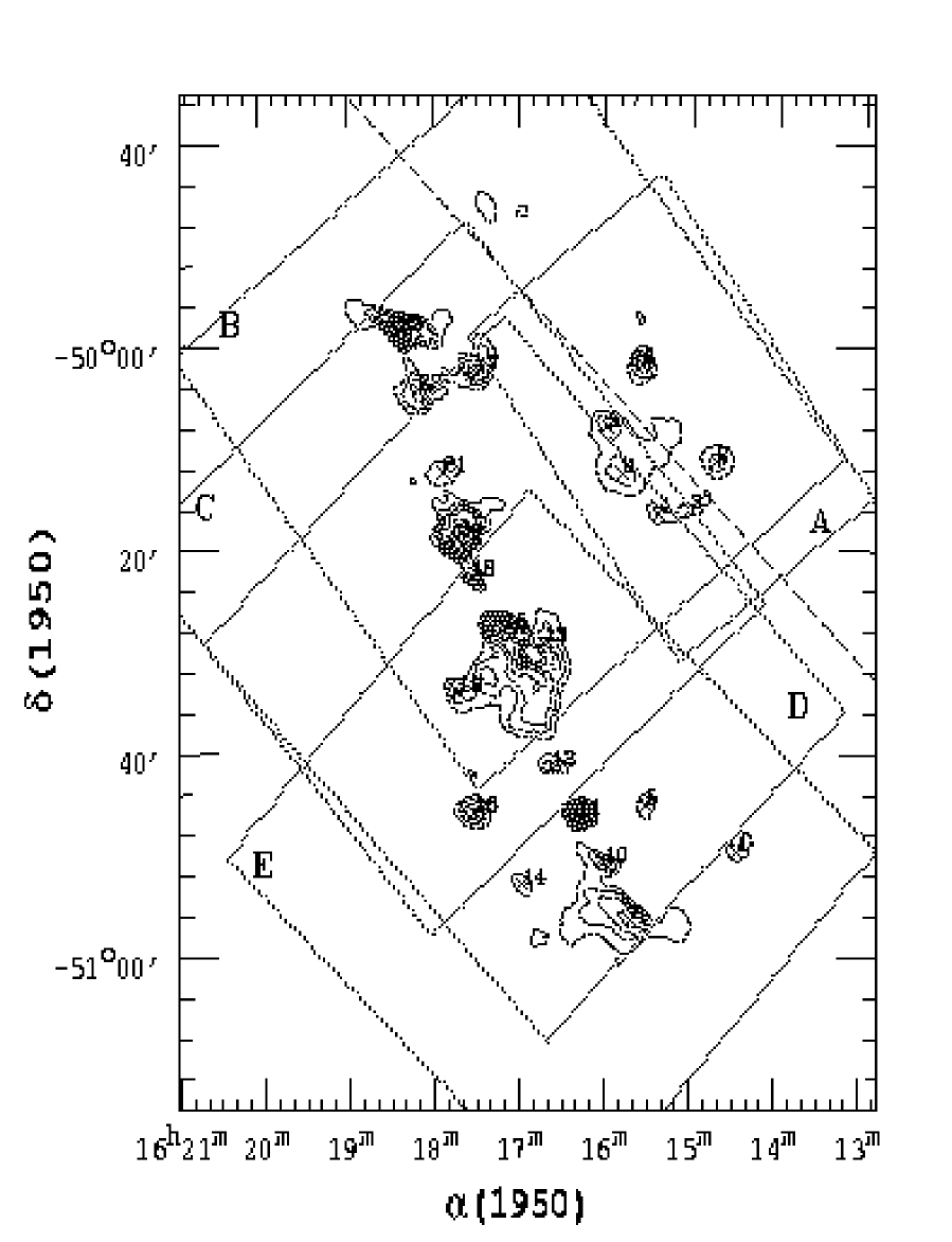
Figure 1: The map of RCW 106 region at 210 µm. Contour levels are drawn at 1, 2.5, 5, 10, 20, 30, 50, 70 and 90 percent of peak intensity (4375 Jy /$\sq\arcmin$ ). The rectangular boxes show the approximate area covered by each of the individual raster scans A, B, C, D and E respectively. The dashed line shows the position of the Galactic plane. The crosses show positions of the detected sources.

2.1 Balloon-borne FIR observations

The observations were carried out on February 20, 1994 using a two band array photometer in the focal plane of the TIFR 1m balloon-borne telescope which was launched from the TIFR Balloon Facility, Hyderabad, India. Details of the telescope and observing procedures have been described by Ghosh et al. (1988). The photometer used has been described by Verma, Rengarajan & Ghosh (1993). It consists of a pair of compact arrays each having 2 $\times$ 3 silicon bolometers cooled to 0.3 K by liquid ³He . The field of view of each detector was $1\aas@@fstack{\prime}6$. The sky was chopped along the cross elevation axis with a throw of $4\aas@@fstack{\prime}2$. Two bands centred around 150 and 210 $\mu$m were obtained by splitting the incoming beam using a cooled dichroic filter and other band limiting filters. The sky viewed in the two bands was almost identical. Jupiter was used for flux calibration as well as for obtaining the point spread function (PSF). A large area of about 1.2 $\sq\hbox{${}^{\circ}$}$ of RCW 106 complex was mapped in five overlapping rasters.

All six detectors of each band were independently calibrated for their responsivity by using in situ measurements of Jupiter. The telescope aspects corresponding to different detectors of each band were reduced to a reference detector using the known relative positions in the focal plane. The responsivity corrected signals (during the mapping observations of the target source), from all detectors of the same band were then gridded into a two dimensional sky matrix ( elevation $\times$ cross elevation; cell size of $0\aas@@fstack{\prime}3$ $\times$ $0\aas@@fstack{\prime}3$). This signal matrix was deconvolved using a procedure based on maximum entropy method (MEM; see Ghosh et al. 1988 for details). The FWHMs of the deconvolved beam for Jupiter were found to be $1\arcmin$ $\times$ 1$\aas@@fstack{\prime}3$ (elevation $\times$ cross elevation) for both bands.

Since our wavelength bands are broad, the flux density estimated from the observed signal is a function of the incident spectrum. Following the IRAS convention we present flux densities for a $\nu f_{\nu}$ = constant spectrum. When computing flux density for other spectral shapes a colour correction is applied such that $f_{\nu}$(actual) = $f_{\nu}$(quoted)/ K. For a gray body spectrum with emissivity $\epsilon\propto\lambda^{-1}$ the K factor at 150 $\mu$m varies from 0.85 to 0.57 as the temperature is varied from 20 K to 60 K; at 210 $\mu$m the variation is from 0.84 to 0.85. For an emissivity $\epsilon\propto\lambda^{-2}$  the corresponding values are 0.7 to 0.52 for the 150 $\mu$m band and 0.81 to 0.87 for the 210 $\mu$m band.

2.2 Pointing accuracy

The absolute pointing accuracy was determined in two different ways. (i) An optical photometer (with a photomultiplier tube as detector) at the cassegrain focal plane of the telescope always views a region of the sky neighbouring the FIR field (Naik et al. 2000). The sky chopped signals obtained from this photometer during the FIR scans across the target source were also MEM deconvolved to generate optical intensity maps of the scanned region. The stars detected in these maps have been used to quantify absolute aspects of our maps. Using 17 well identified and isolated optical stars, the mean deviation and rms were found to be 0$\aas@@fstack{\prime}$2 and 0$\aas@@fstack{\prime}$7 respectively along RA and 0$\aas@@fstack{\prime}$06 and 0$\aas@@fstack{\prime}$68 along the Dec axis. (ii) A similar exercise was carried out using the coordinates of six well isolated FIR sources in the IRAS as well as the TIFR maps. The rms deviations along RA and Dec axes were found to be 0$\aas@@fstack{\prime}45$ and 0$\aas@@fstack{\prime}2$ respectively. It may be mentioned that the FIR signal matrix has a much higher filling factor as compared to the optical signal matrix generated using only a single detector. Thus, our absolute pointing over an area as large as 1.2 $\sq\hbox{${}^{\circ}$}$ observed over an hour is better than 0$\aas@@fstack{\prime}5$.

2.3 IRAS-HIRES maps

The HIRES maps processed from the IRAS data of RCW 106 region were obtained from the Infrared Processing and Analysis Center (IPAC, Caltech). These maps were processed using the maximum correlation method (MCM, Aumann, Fowler & Melnyk 1990). The resolution enhancement results in elliptical beams with FWHMs of $1\aas@@fstack{\prime}$0 $\times$ $0\aas@@fstack{\prime}$45, 0$\aas@@fstack{\prime}$95 $\times$ 0$\aas@@fstack{\prime}$45, 1$\aas@@fstack{\prime}$3 $\times$ 0$\aas@@fstack{\prime}7$, and 1$\aas@@fstack{\prime}$9 $\times$ 1$\aas@@fstack{\prime}$3 at 12, 25, 60 and 100 $\mu$m respectively. The position angle of the major axis of the beam is 100^∘. The overall variation in the beam size in different regions of the map is about 15%.

3 Results

3.1 Intensity maps

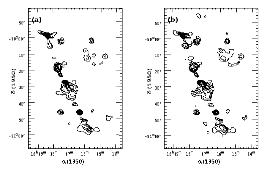
Figure 2: TIFR maps of RCW 106 region for (a) 150 & (b) 210 µm. Contour levels are drawn at 1, 2.5, 5, 10, 20, 30, 50, 70 and 90 percent of peak intensity 9728 and 4375 Jy /$\sq\arcmin$ at 150 and 210 µm respectively.

Fig. 1 shows an enlarged intensity map at 210 $\mu$m obtained from our observations combining all the five rasters. The boundaries of individual raster areas are also shown. The long dashed line shows the position of the Galactic plane. In Fig. 2a and 2b we show the intensity maps at 150 $\mu$m and 210 $\mu$m. The peak flux densities at 150 and 210 $\mu$m are 9728 and 4375 Jy/$\sq\hbox{${}^{\circ}$}$ respectively while the noise is found to be 16 and 9 Jy/$\sq\hbox{${}^{\circ}$}$. The lowest contour level shown is 1% of the peak and is several times the noise. From the figures it is seen that the star formation in RCW 106 is along a narrow ridge roughly parallel to the Galactic plane. It is also seen that the FIR emission is subdivided into five collinear sub complexes.

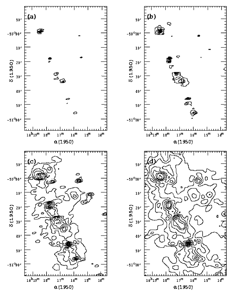
Figure 3: HIRES processed IRAS maps of RCW 106 region at (a) 12, (b) 25, (c) 60 and (d) 100 µm. Contour levels are drawn at 1, 2.5, 5, 10, 20, 30, 50, 70 and 90 percent of peak intensity 4875, 8455, 7947 and 4884 Jy /$\sq\arcmin$ for 12, 25, 60 and 100 µm respectively.

Figs. 3a–d show the IRAS HIRES intensity maps at 12, 25, 60 and 100 $\mu$m. Once again the lowest contour level shown is 1% of the peak. The IRAS maps, especially at 60 and 100 $\mu$m are morphologically similar to our maps. However, we resolve more sources as compared to the IRAS. The FIR maps are also very similar to the radio continuum maps of Goss & Shaver (1970) and Shaver & Goss (1970a).

3.2 Maps of temperature and optical depth

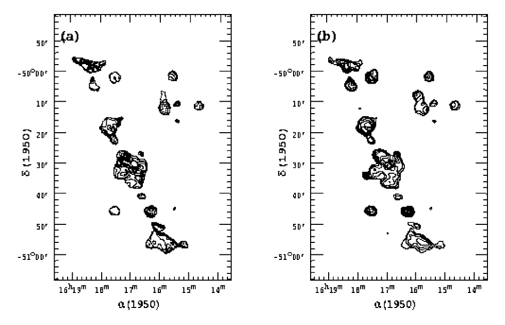
Figure 4: The maps of RCW 106 region for (a) Temperature ($T_{150/210}$) and (b) optical depth at 210 µm. The dust grain emissivity is assumed to be $\propto\nu^{2}$. Contours for temperature are plotted at 20, 24, 28, 32, 36, 40 and 44 K. Contours for optical depth are plotted at 1, 2.5, 5, 10, 20, 30, 50, 70, and 90 percent of peak optical depth of 0.10 .

Far-infrared and sub-millimeter observations can be effectively used to obtain column densities of the region from the optical depth at these wavelengths [Hildebrand 1983]. Recent studies using IRAS data at 60 and 100 $\mu$m have shown that the 100 $\mu$m optical depth correlates well with other column density indicators namely CO and visual extinction (Langer et al. 1989; Jarrett, Dickman & Herbst 1989). Since we have simultaneous observations in two trans-IRAS wavelengths with almost identical FOV, we make use of these maps to derive reliable maps of both the temperature and optical depth. Our longer wavelength coverage also makes our data more sensitive to colder dust (temperature down to about 15 K) as compared to the IRAS coverage. The intensity maps were smoothed by taking average within a box of $0\aas@@fstack{\prime}9\times 0\aas@@fstack{\prime}9$ size and these were, in turn, used to obtain maps of temperature and optical depth. To derive the temperature, we assume an emissivity dependence $\epsilon\propto\lambda^{-2}$ . These are shown in Fig. 4.

The temperature map shows a lot of structure and several high temperature regions near the cloud boundaries. These regions are, most probably, sites of H ii blisters where the dust is heated by radiation from young stars close to the boundary. The optical depth map is morphologically similar to the intensity maps and the peaks in the two coincide indicating presence of high densities near the embedded sources.

Assuming a homogeneous mixture of silicate ($\rho=$ 3.3 g/cm^-3) and graphite ($\rho=$ 2.26 g/cm^-3) dust grains with a power law size distribution (index = $-3.5$) as given by Mathis, Rumpl & Nordsieck (1977) and using the absorption efficiencies as per Laor & Draine (1993), we estimate the total dust mass of the complex to be equal to 1800 M$\odot$. If one takes the gas to dust ratio to be 100, then the total mass of the cloud is $1.8\times 10^{5}$ M$\odot$. This value is typical for a GMC of size of 70 pc in the Galactic plane. However it may be noted that this estimate of cloud mass may be an underestimate, because due to chopping, low gradient diffuse flux is missed in our observations (see next subsection).

3.3 Embedded sources

Flux calibrated maps (Figs. 2a and 2b) were processed to extract discrete sources and to obtain their flux densities. The HIRES processed maps of the IRAS survey data at 12, 25, 60 and 100 $\mu$m were also used to supplement our observations. For all six bands (four IRAS and two of TIFR) the following procedure was adopted to extract sources. For each pixel in the image map, if the pixel value was greater than or equal to a specified threshold then the maximum pixel value within a box of size 5$\times$5 pixels around this pixel was obtained. If the pixel value was equal to this maximum, the position was assumed to be the peak position for a source and its centroid position was determined using the IRAF software. A total of 23 sources were thus found at 210 $\mu$m. More details can be found in Karnik (2000).

The associations of the above sources with sources in other maps viz. , 150 $\mu$m map of TIFR and the IRAS maps at 12, 25, 60 and 100 $\mu$m were searched for, demanding a centroid separation of less than 1$\aas@@fstack{\prime}$0 at 150 $\mu$m and 1$\aas@@fstack{\prime}$5 at other wavelengths. All 23 sources are detected at 150 $\mu$m. Eighteen of the 23 sources have IRAS associations with detection in two or more bands. We have five sources that are detected only in our maps. This is due to the superior resolution of our maps resulting from the smaller FOV. The flux densities of sources detected in each band were obtained using the numerical aperture photometry and an aperture value of 3$\arcmin$ diameter; the sky background was evaluated as mode value within an annulus of $0\aas@@fstack{\prime}5$ width at radius of 4$\arcmin$ and subtracted from each pixel before obtaining the aperture sum. The flux densities obtained at 150 and 210 $\mu$m bands were colour corrected assuming a gray body spectrum with emissivity $\propto\lambda^{-2}$, and a temperature corresponding to the ratio of fluxes in the two bands. The IRAS flux densities were colour corrected assuming a power law type of flux density distribution between two neighbouring bands. The overall errors on the total flux densities including calibration errors are about 15–20%. The colour corrected flux densities along with the source positions in the 210 $\mu$m map are presented in Table 1. The SED of each source was constructed using these tabulated values. The luminosities of the sources were derived by integrating the SED and assuming a distance of 3.6 kpc [Lockman 1979]. Out of band correction based on the T(150/210) was also made. For the five sources which were detected only in our maps the total flux was estimated from the temperature given by the ratio of flux densities and assuming $\epsilon\propto\lambda^{-2}$. For source S23, IRAS signals were saturated at 60 and 100 $\mu$m. We, therefore, estimated these by extrapolation from the 150 and 210 $\mu$m flux densities. The computed luminosities for all the sources are also shown in Table 1.

Table 1: Positions at 210 $\mu$m and other properties of detected sources

Source	R.A.∗	DEC∗	IRAS PSC	Flux Density in Jy†						Lum.	IRE‡
	(1950)	(1950)		12 $\mu$m	25 $\mu$m	60 $\mu$m	100 $\mu$m	150 $\mu$m	210 $\mu$m	103 L$\odot$
S1	16 14 27.6	-50 49 40	–	–	–	–	–	872	326	62	0.461
S2	16 14 43.1	-50 11 21	16148-5011	64.6	208	1822	2648	1357	766	52	–
S3	16 15 01.1	-50 16 02	-	–	140	1229	2253	648	308	32	–
S4	16 15 23.3	-50 16 27	16153-5016	103	140	1229	2253	690	342	38	–
S5	16 15 31.2	-50 45 08	–	52.5	143	1193	1432	653	338	32	–
S6	16 15 34.6	-50 01 46	16156-5002	102	359	2930	3492	2379	1275	82	1.01
S7	16 15 42.1	-50 56 25	16158-5055	331	1732	8140	8158	6373	3079	249	0.551
S8	16 15 48.4	-50 12 29	16159-5012	54.7	257	2611	3801	1910	976	71	0.171
S9	16 15 58.6	-50 07 53	–	–	–	–	–	1332	996	9.8	–
S10	16 16 00.7	-50 50 48	16159-5049	137	503	3200	3713	2050	817	91	–
S11	16 16 18.2	-50 46 08	16164-5046	221	2033	14120	16790	15380	7790	411	1.041
S12	16 16 37.5	-50 41 17	–	–	–	–	–	1073	512	21	–
S13	16 16 43.3	-50 29 09	–	–	–	–	–	2715	1275	56	–
S14	16 16 58.2	-50 52 56	16170-5053	–	203	1338	1485	582	333	31	–
S15	16 17 10.8	-50 27 48	16172-5028	468	3044	12920	18355	20811	10009	482	0.581
S16	16 17 31.5	-50 45 52	16175-5045	–	101	1141	1818	2372	1546	37	–
S17	16 17 31.6	-50 02 20	16175-5002	40.2	177	1833	3201	3198	2132	62	1.502,3
S18	16 17 33.3	-50 22 37	16174-5022	134	600	4019	5576	2180	1043	115	–
S19	16 17 42.9	-50 34 03	–	–	–	–	–	973	1017	5.4	–
S20	16 17 42.9	-50 18 52	16177-5018	417	3164	13207	17243	15572	8015	460	0.721,2
S21	16 17 53.3	-50 12 25	–	–	–	1088	2168	572	456	19	–
S22	16 18 10.4	-50 04 18	-	54.8	214	1970	3940	2194	1524	65	–
S23	16 18 22.9	-49 58 25	16183-4958	3372	12097	12395	16785	27841	11555	921	$>$0.571,2,3

^∗ Units of Right Ascension are hours, minutes and seconds, and the units of Declination are degrees, minutes and seconds.

^† Flux densities are within 3$\arcmin$ diameter.

^‡ References of radio data for calculating IRE are – 1) Shaver & Goss (1970b); 2) Retallack & Goss (1980); 3) Forster et al. (1987).

We estimate the diffuse emission in the complex by subtracting the sum of flux densities of the extracted sources from the total flux density of the map down to 1% contour level. We find the diffuse fraction to be 81%, 84%, 19% and 27% at 60, 100, 150 and 210 $\mu$m respectively. In contrast to the IRAS, our chopped observations are less sensitive to low gradient diffuse flux. The fraction of diffuse flux obtained using chopped observations of RCW 106 complex may be compared with values obtained for other regions using similar chopped observations: $\leq$ 50% for Carina complex [Ghosh et al. 1988], 35% for W 31 [Ghosh et al. 1989b] and 35% for IRAS 09002$-$4732 region [Ghosh et al. 2000] .

3.4 Comparison with radio observations

We have looked for association of the FIR sources with radio continuum sources detected by others, demanding that positions match within $2\aas@@fstack{\prime}0$. We find 10 associations. Taking the FIR luminosity listed in Table 1 as that due to a single ZAMS star, we can estimate the expected rate of emission of Lyman continuum photons. We can also compute the same from the observed radio continuum flux density using the formula of Mezger (1978). We have used the 5000 MHz flux density given by Shaver & Goss (1970b) (at an angular resolution of 4$\arcmin$) wherever available since at this high frequency the radio emission is less affected by optical depth effects. For source S17 we have used the mean of the 1415 MHz flux density of Retallack & Goss (1980) and 1420 MHz flux density of Forster et al. (1987) with an angular resolution $\sim$ 1$\arcmin$ . We have not used very high resolution ($\sim$ 1$\arcsec$) interferometric radio observations of Walsh et al. (1998) as they only give peak flux densities. In Table 1 we present IRE, the ratio of Lyman continuum luminosity derived from the FIR and radio observations. If the radio emission is optically thin and the source is powered by a single ZAMS star, IRE = 1. If however, the energizing source is multiple or if some fraction of Lyman continuum luminosity is absorbed by dust and not available for ionizing the gas, we expect IRE $>$ 1. This can also result if a fraction of the FIR luminosity is due to accretion (Garay & Lizano 1999) since accretion is unlikely to produce energetic Lyman continuum photons. From Table 1 we find that only one source viz., S17 has IRE significantly higher than unity and even for this, it is consistent with unity if 50 % of Lyman continuum photons are unavailable for ionization because of dust absorption (Smith, Biermann & Mezger 1978). For all other sources the ratio is $\leq$ 1; this is most probably due to the fact that the resolution of radio observations used is generally much poorer than that of our FIR observations.

It is generally believed that massive stars are formed in clusters. We may, therefore, have additional unresolved stars within our effective resolution of 1$\aas@@fstack{\prime}2$. However, in the light of IRE discussed above, we cannot make definite statement about the presence of multiple sources. We can only conclude that another massive star with a significant fraction of observed luminosity is unlikely to be present. Similar statement can also be made for luminosity from accretion.

4 Stellar Luminosity Distribution and Initial Mass Function

For deeply embedded objects like the RCW 106, the FIR luminosity is almost the bolometric luminosity of the energizing star(s). Making use of the 23 objects detected by us, we construct the stellar luminosity distribution of massive stars in the RCW 106 complex. This is shown in Fig. 5. From an inspection of the figure we see that our sampling is nearly complete for L $>$ 20,000 L$\odot$. Assuming the luminosity distribution to be a power law given by N[log (L/L$\odot$)] $\propto$ $\alpha$ log (L/L$\odot$) and using the more robust (as compared to binning) maximum likelihood method, we find $\alpha$ = $-0.67\pm 0.22$ for L $>$ 20,000 L$\odot$. It may be noted that due to factors discussed in the previous section, the observed distribution could be flatter than the intrinsic one. Our value of slope may be compared with the value of $-0.56$ derived by Rengarajan (1984) from the M17SW data of Jaffe, Stier & Fazio (1982).

Figure 5: Luminosity distribution for sources in RCW 106 region. The line shows the fit obtained using maximum likelihood method assuming power law type of number distribution.

The initial mass function (IMF) of stars is usually defined as the birth rate of stars formed per unit logarithmic mass interval per unit time. The shape of the IMF ($\xi(log~{}m_{*})$) is generally characterized as a power law with a spectral index ($\beta$). The IMF at birth is normally derived from the observed present day mass function (PDMF) and applying corrections to it. For example, the well known Salpeter IMF [Salpeter 1955] and Miller Scalo IMF [Miller & Scalo 1979] are derived from the population of field stars after correcting for life times, scale heights etc. These estimates are, therefore, averaged over a large volume and over the life of the Galaxy. In a recent review Scalo (1998) summarises the more accurate spectroscopic observations of massive stars in clusters and associations (age up to a few million years) and concludes that there is a large uncertainty in the value of $\beta$ and that it ranges between $-1$ and $-$2. An interesting question is what is the shape of IMF at a very early stage when stars are still deeply embedded in molecular clouds? The large number of high mass stars observed in the RCW complex and a young age ($<$ 100,000 years) give us an opportunity to study the IMF at birth. For this purpose, the FIR luminosities were used to obtain masses using the mass–luminosity relation for a ZAMS star with solar metallicity, using the analytical relation given by Tout et al. (1996). Again using the maximum likelihood method we find $\beta$ = $-1.73\pm 0.5$ for mass $\geq$ 15 M$\odot$. As is the case for the luminosity distribution, the actual IMF would be steeper. This slope is in the same region as the values determined for massive stars and for stars of intermediate mass from photometric observations of stellar clusters (Scalo 1998). Ghosh et al. (2000) obtained $\beta$ = $-1.25$ in the mass range of 4–16 M$\odot$ in the complex around IRAS 09002$-$4736. Okumura et al. (2000) using near infrared imaging observations of W51 find that the slope above 10 M$\odot$ is consistent with $-1.8$ and perhaps flattens above 30 M$\odot$.

5 Radiation Transfer Modelling

5.1 Modelling Procedure

Table 2: Parameters^∗ for the models shown in Figures 6 and 7

	Best fit					Second best fit						Poorest fit
Source	R	Rc	$\gamma$	$\tau_{100}$	fsil	R	Rc	$\gamma$	$\tau_{100}$	fsil	$\chi^{2\dagger}$	R	Rc	$\gamma$	$\tau_{100}$	fsil	$\chi^{2\dagger}$
	(pc)	(pc)				(pc)	(pc)					(pc)	(pc)
S2	0.64	0.017	1	0.19	0.13	0.68	0.009	0	0.06	0.66	1.0	0.60	0.064	2	0.17	0.10	4.7
S4	0.26	0.016	1	0.21	0.00	0.38	0.008	0	0.07	0.23	1.3	0.30	0.034	2	0.20	0.00	1.8
S5	0.37	0.006	0	0.07	0.39	0.39	0.018	1	0.16	0.16	1.4	0.38	0.040	2	0.16	0.10	2.9
S6	0.81	0.009	1	0.25	0.07	1.04	0.013	0	0.05	0.89	6.1	0.90	0.087	2	0.17	0.06	40.0
S7	2.14	0.038	1	0.10	0.33	1.22	0.028	0	0.06	0.56	5.4	1.10	0.153	2	0.12	0.05	6.8
S8	0.56	0.021	1	0.22	0.12	0.61	0.009	0	0.09	0.55	1.7	0.44	0.070	2	0.20	0.09	5.7
S10	0.58	0.021	0	0.07	0.45	0.87	0.026	1	0.11	0.28	1.5	0.56	0.009	2	0.13	0.14	3.7
S11	2.62	0.054	1	0.18	0.10	2.08	0.182	0	0.09	0.40	1.5	2.77	0.168	2	0.18	0.07	11.0
S15	4.36	0.051	1	0.15	0.20	2.42	0.017	0	0.08	0.47	7.6	2.13	0.219	2	0.13	0.06	11.0
S17	1.24	0.016	0	0.11	0.48	1.06	0.040	1	0.25	0.08	4.6	0.72	0.146	2	0.22	0.06	22.6
S18	0.69	0.022	1	0.15	0.18	0.69	0.016	0	0.06	0.75	1.2	0.50	0.093	2	0.14	0.95	1.8
S20	4.32	0.063	1	0.11	0.36	1.93	0.010	0	0.07	0.51	19.0	1.13	0.212	2	0.16	0.10	24.3
S22	0.78	0.024	1	0.27	0.06	0.84	0.014	0	0.10	0.47	1.3	1.76	0.083	2	0.22	0.03	12.2

^∗For each source three sets of parameters are given. These are for the best fit models for each of the three types of density distributions. The order among the three sets is according to the fit. Thus the first set corresponds to the best fit out of the three, the last corresponds to the poorest fit. The parameters are – R, the radius of the cloud, R_c the radius of the central dust free cavity, $\gamma$, the power law index of the radial density distribution [$\rho(r)\propto r^{-\gamma}$], $\tau_{100}$, the radial optical depth at 100 $\mu$m and f_sil, the fractional abundance of silicate.

${}^{\dagger}\chi^{2}$ values are given relative to the best fit (i.e. $\chi^{2}_{\rm Second~{}best~{}fit}/\chi^{2}_{\rm Best~{}fit}$ and $\chi^{2}_{\rm Poorest~{}fit}/\chi^{2}_{\rm Best~{}fit}$ ).

The emergent SED of an embedded source depends on the luminosity of the source and the physical properties of its dusty envelope. By fitting the observed SED to radiation transfer calculation, one can obtain useful information on the geometric details and nature of dust. With this in mind we have chosen, from Table 1, thirteen sources that have measured flux densities in all six bands, viz. , the two TIFR and four IRAS bands. The source S23 was excluded as the IRAS signals at 60 and 100 $\mu$m are saturated. The radiation transfer calculation was carried out through a purely dust component in a spherical geometry using the code CSDUST3 [Egan, Leung and Spagana 1988]. The central source was assumed to be a single star with a luminosity equal to the value derived from observations. A mixture of graphite and astronomical silicate with properties as given by Laor & Draine (1993) was assumed. Size distribution [$n(a)$] was assumed to be a power law [$n(a)\propto a^{-3.5}$] as per Mathis et al. (1977). The free parameters of the model were – R, the size of the envelope , R_c, the size of the central dust free cavity , $\tau_{100}$, the total (due to both type of grains) radial optical depth at 100 $\mu$m, $f_{sil}$ , the fractional abundance of silicate and $\gamma$, the power law index of the radial density distribution within the envelope [$\rho(r)\propto r^{-\gamma}$]. Only three discrete values of 0, 1 and 2 were explored for $\gamma$. A $\chi^{2}$ minimization scheme was developed for fitting the computed SED of the model to the observed SED of the source and the fitting was done for each value of $\gamma$.

The sensitivity of the $\chi^{2}$ minimization scheme in terms of extracting the parameters (mainly for index $\gamma$) accurately from the input observed SED of the source was tested using simulation. Synthetic input was created by calculating the flux densities at the six wavelengths used as well as in the NIR (5 $\mu$m) and sub-mm (800 $\mu$m) with added random noises. From the results of the simulation we conclude that i) the best fit always corresponds to the case when the $\gamma$ value is the same for the input spectrum and the modelled spectrum; presence of NIR point improves the discrimination especially for $\gamma$ = 1 or 2; ii) the radius of the central dust free cavity and optical depth at 100 $\mu$m are the most sensitive parameters of the modelling procedure, the variation between the input parameters and the extracted parameters for both is about 20%, while for the outer radius it is about 30%; iii) the dust composition is a parameter with poor extraction accuracy since the absorption efficiency beyond about 50 $\mu$m is the same for graphite and silicate and the main constraints come from data points at 25 $\mu$m or lower.

5.2 Results of modelling RCW 106 sources

Figure 6: Spectral energy distribution for the six sources S7, S10, S5, S11, S2 and S4 in RCW 106 complex region as given in Table 1. The lines shown are fits from radiation transfer models. Different lines depict fits for three different power law dependence of radial density. The parameters for these fits are given in Table 2. Note that for the sake of clarity flux densities have been multiplied by a different constant factor for five of the sources.

Figure 7: SED plots similar to those in Fig. 6, but for sources S15, S8, S18, S6, S20, S17 and S22.

Figures 6 and 7 show the observed data points and the best fit SED for each value of $\gamma$ for the 13 selected sources. The parameters of these models, along with relative $\chi^{2}$ values, are presented in Table 2.

Table 3: Density distribution near embedded high mass stars

$Resolution$	$\gamma$	Reference
$1\aas@@fstack{\prime}2$	0 or 1	(FIR) Present work, Ghosh et al. (2000),
		Mookerjea et al. (1999,2000)
$0\aas@@fstack{\prime}5$	0 or 1	(FIR) [Campbell et al. 1995]
$0\aas@@fstack{\prime}15$	0	(MIR) [Faison et al. 1998]
$0\aas@@fstack{\prime}15$/$0\aas@@fstack{\prime}25$	1.5	(Sub-mm) [Hatchell et al. 2000]
$0\aas@@fstack{\prime}5$	2–1	(Sub-mm) [Hunter 1997]

From Figs. 6, Fig. 7 and Table 2 it is seen that for 9 out of the 13 sources $r^{-1}$ distribution fits the SED best while for the rest, uniform distribution is the best fit. It may be mentioned that there is not much difference between the the final $\chi^{2}$ obtained for the best fits for the two density distributions. The $r^{-2}$ distribution shows the poorest fit for all sources. Table 3 lists the radial distribution index obtained in recent times by different authors using radiation transfer modelling of envelopes of high mass embedded sources. This compilation suggests that in many cases the density distribution differs from $\rho(r)\propto r^{-2}$ or $r^{-1.5}$ that is expected for the envelopes of young protostars [Shu, Adams & Lizano 1987]. Is there really a lack of sources with $r^{-2}$ density distribution as revealed by FIR and MIR observations? This can be checked only through higher angular resolution observations at FIR wavelengths and modelling actual radial intensity profiles. However, there is no prospect of large improvement of angular resolution in the FIR in the near future. If the density distribution is indeed different from that expected for free fall models (i.e. $\propto r^{-2}$), what are the possible reasons for this? Do high velocity outflows arising from young high mass stars and radiation pressure on dust grains due to intense UV radiation from the young high mass star help in modifying the initial free fall density distribution $\propto r^{-2}$ ? Jijina & Adams (1996), accounting for effect of radiation pressure, predict that close to the star, density distribution should be $\propto r^{-0.5}$ and at larger distances $\propto r^{-1.5}$. One should note that these solutions are at much smaller scales compared to those sampled by the large beams of most of the FIR observations.

5.3 Luminosity and Envelope Mass

Figure 8: The FIR luminosity of the source plotted against the mass of the dust envelope obtained from the best fit radiation transfer model. The solid line represents the power law regression fit to the points.

The mass computed from the best fit model parameters represents the mass of the star forming envelope if one assumes a constant gas to dust ratio. In Fig. 8 the luminosity of the source is plotted against the computed dust mass of the envelope. A correlation is seen between the two. The probability of finding no correlation is as low as 0.0086. The power law index after regression analysis is found to be $0.7\pm 0.11$. This indicates that the more massive molecular cores produce more massive stars.

6 Summary

The star forming region associated with RCW 106 has been mapped simultaneously at 150 and 210 µm. The HIRES processed IRAS survey data are used as supplement to our data. The temperature and the FIR optical depth maps have been generated for the region. The total dust mass estimated from the optical depth map is about 1800 M$\odot$. The local maxima in the 210 µm map have been searched for to find the embedded sources. The associations of these sources are found in the four IRAS maps and the 150 µm map. The diffuse fraction in these maps is found to be 81% and 84% in the IRAS 60 and 100 µm bands while it is 19% and 27% at 150 and 210 µm from our chopped observations. The SEDs for the sources are constructed and FIR luminosities estimated. Luminosity distribution of these sources has been obtained. These FIR luminosities are used, along with mass-luminosity relation for ZAMS stars, to obtain IMF of the region. The estimated power law index of IMF is $-1.73$ for mass $\geq$ 15 M$\odot$  similar to that of other star forming regions and OB associations albeit flatter than the IMF for field stars. The SEDs of the sources detected in all the bands are modelled using radiation transfer calculations assuming a dusty envelope surrounding the young ZAMS star with luminosity equal to that of the FIR luminosity of the source. The size of the envelope, inner dust free core radius, line of sight optical depth due to dust at 100 $\mu$m and composition of the dust were varied to obtain the best fit to the observed SED. Three types of radial density distributions – [$\rho(r)\propto r^{-n}$ where $\gamma$=0, 1 and 2] were tried for. The best fit results show that $r^{-2}$ can be ruled out against uniform and $r^{-1}$ distributions. A correlation was found between the the source luminosity and the mass of dusty envelopes calculated using the best fit model parameters.

Acknowledgements

We thank S.L. D’Costa, M.V. Naik, S.V. Gollapudi, D.M. Patkar, M.B. Naik and G.S. Meshram for their support for the experiment. The members of TIFR Balloon Facility (Balloon group and Control & Instrumentation group), Hyderabad, are thanked for their roles in conducting the balloon flights. IPAC is thanked for providing HIRES processed IRAS data. TNR thanks JSPS and Dr. H. Shibai for the Invitation Fellowship at the Physics Department, Nagoya University where part of this work was done.

References

- [Aumann et al. 1990] Aumann H. H., Fowler J. W., Melnyk M., 1990, AJ, 99, 1674
- [Batchelor et al. 1980] Batchelor R. A., Caswell J. L., Haynes R. F., Wellington K. J., Goss W. M., Knowles S. H., 1980, Australian Journal of Physics, 33, 139
- [Batchelor et al. 1977] Batchelor R. A., Gardner F. F., Knowles S. H., Mebold U., 1977, Proceedings of the Astronomical Society of Australia, 3, 152
- [Braz et al. 1989] Braz M. A., Gregorio Hetem J. C., Scalise J., E., Monteiro Do Vale J. L., Gaylard M., 1989, A&AS, 77, 465
- [Braz & Scalise 1982] Braz M. A., Scalise J. E., 1982, A&A, 107, 272
- [Campbell et al. 1995] Campbell M. F., Bunter H. M., Harvey P. M., Evans II N. J., Campbell M. B., Sabbey C. N., 1995, ApJ, 454, 831
- [Caswell & Haynes 1975] Caswell J. L., Haynes R. F., 1975, MNRAS, 173, 649
- [Caswell, Haynes & Goss 1980] Caswell J. L., Haynes R. F., Goss W. M., 1980, Australian Journal of Physics, 33, 639
- [Caswell et al. 1995] Caswell J. L., Vaile R. A., Ellingsen S. P., Norris R. P., 1995, MNRAS, 274, 1126
- [Egan, Leung and Spagana 1988] Egan M. P., Leung C. M., Spagana G. F., 1988, Computer Physics Communications, 48, 271
- [Ellingsen et al. 1996] Ellingsen S. P., Von Bibra M. L., McCulloch P. M., Norris R. P., Deshpande A. A., Phillips C. J., 1996, MNRAS, 280, 378
- [Faison et al. 1998] Faison M., Churchwell E., Hofner P., Hackwell J., Lynch D. K., Russel R. W., 1998, ApJ, 500, 280
- [Forster et al. 1987] Forster J. R., Whiteoak J. B., Kestevan M. J., Manchester R. N., Rayner P. T., Ables J. G., Peters W. L., 1987, MNRAS, 226, 173
- [Gardner & Whiteoak 1978] Gardner F. F., Whiteoak J. B., 1978, MNRAS, 183, 711
- [Gardner & Whiteoak 1984] Gardner F. F., Whiteoak J. B., 1984, MNRAS, 210, 23
- [Garay & Lizano 1999] Garay G., Lizano S., 1999, PASP, 111, 1049
- [Ghosh et al. 1988] Ghosh S. K., Iyengar K. V. K., Rengarajan T. N., Tandon S. N., Verma R. P., Daniel R. R., 1988, ApJ, 330, 928
- [Ghosh et al. 1989a] Ghosh S. K., Iyengar K. V. K., Rengarajan T. N., Tandon S. N., Verma R. P., Daniel R. R., 1989a, ApJS, 69, 233
- [Ghosh et al. 1989b] Ghosh S. K., Iyengar K. V. K., Rengarajan T. N., Tandon S. N., Verma R. P., Daniel R. R., Ho P. T. P., 1989b, ApJ, 347, 338
- [Ghosh et al. 1990] Ghosh S. K., Iyengar K. V. K., Rengarajan T. N., Tandon S. N., Verma R. P., Daniel R. R., 1990, ApJ, 353, 564
- [Ghosh et al. 2000] Ghosh S. K., Mookerjea B., Rengarajan T. N., Tandon S. N., Verma R. P., 2000, A&A, 363, 744
- [Gillespie et al. 1977] Gillespie A. R., Huggins P. J., Sollner T. C. L. G., Phillips T. G., Gardner F. F., Knowles S. H., 1977, A&A, 60, 221
- [Goss & Shaver 1970] Goss W. M., Shaver P. A., 1970, Aust. J. Phys. Astrophys. Suppl., No. 14, 1
- [Hatchell et al. 2000] Hatchell J., Fuller G. A., Miller T. J., Thompson M. A., Macdonald G. H., 2000, A&A, 357, 637
- [Hildebrand 1983] Hildebrand H., 1983, QJRAS, 24, 267
- [Hunter 1997] Hunter T. R., 1997, Ph.D. thesis, California Institute of Technology
- [Jaffe et al. 1980] Jaffe D. T., Stier M. T., Fazio G. G., 1982, ApJ, 252, 601
- [Jarrett et al. 1989] Jarrett T. H., Dickman R. L., Herbst W., 1989, ApJ, 345, 881
- [Jijina & Adams 1996] Jijina J., Adams F. C., 1996, ApJ, 462, 874
- [Karnik 2000] Karnik A.D., 2000, Infrared observations of star forming regions, Ph D thesis, University of Bombay, Bombay
- [Kaufmann et al. 1977] Kaufmann P., Scalise J. E., Schaal R. E., Gammon R. H., Zisk S., 1977, AJ, 82, 577
- [Langer et al. 1989] Langer W. D., Wilson R. W., Goldsmith P. F., Beichman C. A., 1989, ApJ, 337, 355
- [Laor & Draine 1993] Laor A., Draine B. T., 1993, ApJ, 402, 441
- [Lockman 1979] Lockman F. J., 1979, ApJ, 232, 761
- [Macleod & Gaylard 1992] Macleod G. C., Gaylard M. J., 1992, MNRAS, 256, 519
- [Macleod et al. 1998] Macleod G. C., van der Walt D. J., North A., Gaylard M. J., Galt J. A., Moriarty-Schieven G. H., 1998, AJ, 116, 2936
- [Mathis, et al. 1977] Mathis J. S., Rumpl W., Nordsieck K. H., 1977, ApJ, 217, 425
- [Mezger 1978] Mezger P. G., 1978, A&A, 70, 565
- [Miller & Scalo 1979] Miller G. E., Scalo J. M., 1979, ApJS, 41, 513
- [Mookerjea et al. 1999] Mookerjea B., Ghosh S.K., Karnik A.D., Rengarajan T.N., Tandon S.N., Verma R.P., 1999, ApJ, 522, 285
- [Mookerjea et al. 2000] Mookerjea B., Ghosh S.K., Rengarajan T.N., Tandon S.N., Verma R.P., 2000, ApJ, 539, 775
- [Naik et al. 2000] Naik M.V., D’Costa S.L., Ghosh S.K., Mookerjea B., Ojha D.K., Verma R.P., 2000, PASP, 112, 273
- [Okumura et al. 2000] Okumura S., Mori A., Nishihara E., Watanabe E., Yamashita T., 2000, ApJ, 543, 799
- [Rengarajan 1984] Rengarajan T. N., 1984, ApJ, 287, 671
- [Retallack & Goss 1980] Retallack D. S., Goss W. M., 1980, MNRAS, 193, 261
- [Rodgers et al. 1960] Rodgers A. W., Campbell C. T., Whiteoak J. B., 1960, MNRAS, 121, 103
- [Salpeter 1955] Salpeter E. E., 1955, ApJ, 121, 161
- [Scalise et al. 1989] Scalise J., E., Rodriguez L. F., Mendoza-Torres E., 1989, A&A, 221, 105
- [Scalo 1998] Scalo J. M., 1998, in Stellar Initial Mass Function, ASP Conference Series, Vol. 142, 201
- [Schutte et al. 1993] Schutte A. J., van der Walt D. J., Gaylard M. J., Macleod G. C., 1993, MNRAS, 261, 783
- [Shaver & Goss 1970] Shaver P. A., Goss W. M., 1970a, Aust. J. Phys. Astrophys. Suppl., No. 14, 77
- [Shaver & Goss 1970b] Shaver P. A., Goss W. M., 1970b, Aust. J. Phys. Astrophys. Suppl., No. 14, 133
- [Shu, Adams & Lizano 1987] Shu F. H., Adams F. C., Lizano S., 1987, ARAA, 25, 23
- [Smith & et al. 1978] Smith L. F., Biermann P., Mezger P.G., 1978, A&A, 66, 65
- [Tout et al. 1996] Tout C. A., Poles O. R., Eggleton P. P., Han Z., 1996, MNRAS, 281, 257
- [van der Walt et al. 1995] van der Walt D. J., Gaylard M. J., Macleod G. C., 1995, A&AS, 110, 81
- [van der Walt et al. 1996] van der Walt D. J., Retief S. J. P., Gaylard M. J., Macleod, G. C., 1996, MNRAS, 282, 1085
- [Verma et al. 1994] Verma R. P., Bisht R. S., Ghosh S. K., Iyengar K. V. K., Rengarajan T. N., Tandon S. N., 1994, A&A, 284, 936
- [Verma et al. 1993] Verma R. P., Rengarajan T. N., Ghosh S. K., 1993, Bulletin of the Astronomical Society of India, 21, 489
- [Walsh et al. 1998] Walsh A. J., Burton M. G., Hyland A. R., Robinson G., 1998, MNRAS, 301, 640