SX Phœnicis Stars in the Core of 47 Tucanae

Abstract

We present new results on five of six known SX Phœnicis stars in the core of the globular cluster 47 Tucanae. We give interpretations of the light curves in the $V$ and $I$ bands from 8.3 days of observations with the Hubble Space Telescope near the core of 47 Tuc. The most evolved SX Phe star in the cluster is a double-mode pulsator (V2) and we determine its mass to be $(1.54\pm 0.05)\,M_{\odot}$ from its position in the Hertzsprung-Russell diagram and by comparing observed periods with current theoretical pulsation models. For V14 we do not detect any pulsation signal. For the double-mode pulsators V3, V15, and V16 we cannot give a safe identification of the modes. We also describe the photometric techniques we have used to extract the light curves of stars in the crowded core. Some of the SX Phœnicis are saturated and we demonstrate that even for stars that show signs of a bleeding signal we can obtain a point-to-point accuracy of 1-3%.

1 Introduction

Blue straggler stars (BSS) are found in all globular clusters where thorough searches for them have been made (Bailyn bailyn (1995)). BSS are thought to be the results of direct collisions between stars or perhaps the gradual coalescence of binary stars (Guhathakurta et al. guha98 (1998), Bailyn bailyn (1995)). The BSS are hotter and brighter than the turn-off stars in a globular cluster and some BSS will cross the classical instability strip for $\delta$ Scuti stars. The variable globular cluster BSS are called SX Phœnicis (SX Phe) stars, using the name for the prototype population II field star.

Table 1: Fundamental parameters for 47 Tucanae. Values are taken from VandenBerg (vandenberg2000 (2000))

[Fe/H]	$E(B-V)$	Age [Gyr]	$V_{TO}$	$(m-M)_{V}$
$-0.83$	$0.032$	$11.5$	$17.65$	$13.37$
$\pm 0.10$	$\pm 0.005$	$\pm 0.8$	$\pm 0.10$	$\pm 0.05$

When discussing globular clusters it is important to realize that they are not just a large group of individual independent stars. BSS are but one piece of evidence for non-standard stellar evolution due to dynamical processes (Camilo et al. pulsars47 (2000), Bailyn bailyn (1995)). For the past five years a number of globular cluster cores have been probed to look more closely at the populations of stars that are direct evidence that the dynamics of stars have influence on the evolution of globular clusters as a whole. This is possible with the Hubble Space Telescope (HST) and has indeed yielded some interesting surprises: 1) BSS are found in all globular clusters (Bailyn bailyn (1995)). 2) The horizontal-branch morphology possibly depends on the dynamical evolution of the cluster, although the metallicity is the most important parameter (Fusi Pecci et al. horizbranch (1996)). 3) The discovery of cataclysmic variables in NGC 6397 (Cool et al. cool (1998)).

BSS and in turn SX Phe stars are found primarily near the cluster core as a result of mass segregation (see e.g. Edmonds et al. edmonds (1996)). With the exceptional resolving power of HST it is possible to probe the cores of globular clusters, examples of such research are 47 Tuc (Gilliland et al. gill98 (1998)) and M5 (Drissen & Shara drissen (1998)) — but see also Piotto et al. (glob-cores (1999)).

1.1 Variable stars in 47 Tuc

The globular cluster 47 Tucanae is one of several clusters which have been searched for binaries and variable stars with the HST. Early results showed that 47 Tuc contained a significant number of BSS (Guhathakurta et al. guha92 (1992)). With observations carried out with the uncorrected optics of HST (September 1993) a study of variable stars in 47 Tuc was made by Edmonds et al. (edmonds (1996)). In this search a few SX Phe and several eclipsing binaries were found (Edmonds et al. edmonds (1996)) as well as variable K giant stars (Edmonds & Gilliland kgiants (1996)).

In particular the BSS were analyzed by Gilliland et al. (gill98 (1998)) who found six SX Phe stars. From the location of the double-mode variables in the Petersen diagram (Petersen & Christensen-Dalsgaard otzen96 (1996)) Gilliland et al. (gill98 (1998)) were able to estimate the pulsation masses for the four double-mode SX Phe stars. Indeed, they showed that the pulsation masses and the evolutionary masses, which were estimated from the positions in the HR diagram, agreed quite well. Combining these two methods of weighing stars, they found masses from $(1.35\pm 0.1)$ to $(1.6\pm 0.2)\,M_{\odot}$ well above the turn-off mass at $\approx 0.85\,M_{\odot}$ in agreement with the generally accepted merging or colliding star scenario for BSS (Bailyn bailyn (1995)).

1.2 Asteroseismology of SX Phe stars

Among the SX Phe stars the double-mode pulsators are particularly interesting. In some cases it is possible to identify the pulsation modes. This class of star is comparable to the classical double-mode Cepheids (Petersen & Christensen-Dalsgaard otzen96 (1996)). The SX Phe stars are often pulsating in the fundamental mode and the first overtone or perhaps in two modes of higher overtones (second and third, third and fourth, etc.). Detections of double-mode SX Phe oscillation have been made in 47 Tuc (Gilliland et al. gill95 (1995, 1998)), $\omega$ Cen (Freyhammer et al. omegacen (1998)), and in a few field variables including SX Phe itself (e.g. Garrido & Rodriguez garrido (1996)).

The observed period ratio and the period of the main mode depend quite sensitively on the mass, metallicity, and evolutionary stage of the star (i.e. the age for a given mass). The ratio of the periods of the double-mode pulsators are well determined from theoretical models: As discussed in Section 5.4 below, the intrinsic precision of the theoretical period ratio is better than $0.01$ percent (see also Petersen & Christensen-Dalsgaard otzen96 (1996)). Hence it is certainly possible to infer physical properties of the double-mode SX Phe stars.

There is evidence that some observed SX Phe stars oscillate in non-radial modes and it may become possible to extract information about the properties of the cores of these stars. Examples of observed SX Phe stars that show evidence of non-radial modes are SX Phe itself (Garrido & Rodriguez garrido (1996)) and V3 in 47 Tuc (Gilliland et al. gill98 (1998)). Progress in the understanding of SX Phe stars can also be made if one can detect low-amplitude modes, which may provide more detailed information about the internal structure of these stars.

Section 2 contains a description of the data set. In Section 3 we discuss the reduction of the data including the task of dealing with saturated bleeding pixels on the CCD. Section 4 contains the details of the time-series analysis while in Section 5 we present the results with emphasis on the double-mode SX Phe stars. Finally, Section 6 summarizes our conclusions.

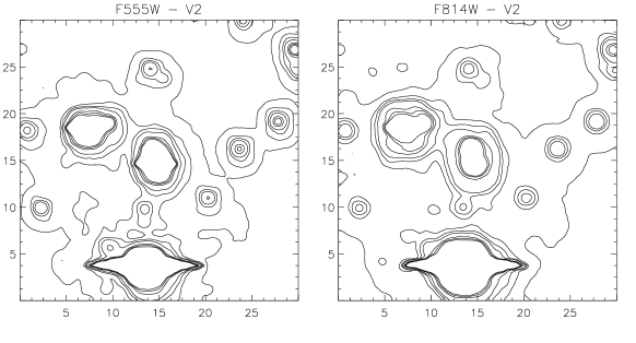
Figure 1: Contour plots around the SX Phe star V2 in the super frame with the F555W and F814W filter. V2 is at position (15,15) and is clearly contaminated by another bright star above it (15,16). In F555W it can be seen that both stars are bleeding in the horizontal (CCD read-out) direction

2 Observations

In the present work we have analyzed an 8.3 day time series of the stars in the central part of 47 Tuc. The data were obtained with WFPC2 on the HST in July 1999. The main goal of the project was to search for giant planets around the main-sequence stars of the cluster (Gilliland et al. gill2000 (2000)). The primary exposure times were 160 s in F555W and F814W filters ($V$ and $I$) and optimized for stars at and below the turn-off. Consequently, the luminous BSS stars are all saturated in $V$ and some are also saturated in $I$.

The PC1 CCD of WFPC2 was placed near the center of 47 Tuc. This is where the density of stars is highest and most of the BSS stars are found. Five of the six known SX Phe stars in the core of 47 Tuc (Gilliland et al. gill98 (1998)) are within the field of view (V1 fell outside).

The present study is an improvement compared to the results by Gilliland et al. (gill98 (1998)). They used HST photometry (with the aberrated WF/PC) in the $U$ band with a total coverage of 39 hours. Although ideal for the detection of stellar oscillations the exposure time was 1000 s compared to 160 s for the present data set. The new time series are more than five times longer with total of 1289 data points compared to the 99 points in the old data set. Although the amplitudes are about a factor of two smaller (using $V$ and $I$ instead of $U$) for the present data set and some of the stars are saturated, we expect to be able to derive more accurate periods for the SX Phe stars.

3 Data reduction

We have used the DAOPHOT/ALLSTAR (D-A) software which is designed for doing photometry in crowded fields (Stetson daophot-art (1987)). For this study we have only reduced the PC1 frames as the BSS stars are found near the core of 47 Tuc. We use D-A to construct an empirical PSF model from about 60 stars. Because of the extreme crowding near the core of 47 Tuc this is a difficult task. The PSF model is iteratively improved by cleaning the neighbouring stars around the stars used for creating the PSF model.

It is well known that the PSF changes with time due to the breathing of HST (Suchkov & Casertano breathing (1997)). We also need a good description of the PSF wings as this has serious impact on the accuracy of the photometry of the saturated SX Phe stars: For these stars the light in the core is not used in the D-A analysis, and we have to look for oscillations in the wings of the PSF profile. Thus we constructed empirical PSF models for all frames.

Figure 2: Difference in internal standard deviation of light curves for two different reduction techniques for the $I$ (left) and $V$ (right) filters. A significant improvement is obtained for the brightest stars

To improve the photometry we have stacked all the frames in each filter to create a super frame. This technique is described in Gilliland et al. (gill99 (1999)). In this way we are able to combine the information from all frames to obtain accurate positions of the stars in each individual frame. This is done by calculating the offset position from the stars in the super frame to each individual frame from the position of several hundred reasonably isolated and bright stars. In order to be able to account for geometric distortion, we find the six coefficients ($a_{1}$ - $a_{6}$) in the transformation

$$X_{i}=a_{1}+a_{2}\,x_{i}+a_{3}\,y_{i}+a_{4}\,x_{i}^{2}+a_{5}\,y_{i}^{2}+a_{6}\,x_{i}\,y_{i}$$

for each frame; here ($x,y$) is the position in the super frame for star $i$, and $X$ is the horizontal position on a given frame. The same is done for the $Y$ coordinate.

We then redo the D-A photometry with the improved positions of the stars being fixed; thus the magnitudes are the only parameters which are fitted by D-A. This step greatly improves the photometric accuracy.

Figure 3: The final internal standard deviation of light curves for the $I$ (left) and $V$ (right) filters. The SX Phe stars have been clearly marked

3.1 Bleeding pixels

We find that the photometry of the brightest saturated stars is quite poor. By inspecting contour levels around stars with different degrees of saturation it is obvious that the signal from the saturated core starts to bleed along the read-out direction. Thus the stellar profile is slightly elongated, i.e. the nice symmetry of the PSF is broken due to the contamination from the bleeding pixels. A specific example of bleeding stars is shown in Figure 1. Note that the data analyzed here have been rotated by 90 degrees from normal WFPC2 conventions, hence bleeding along $x$. We assume that the signal in pixels that are neighbours to saturated cores may not be reliable. To correct for this we used different methods to find the pixels that were affected. It turned out that a simple correction gave good results: We have found that the contamination due to bleeding pixels seems to set in at a certain degree of saturation, i.e. stars for which only the central one or two pixels are saturated do not suffer from contamination. The best result was obtained by flagging pixels which are neighbours to three or more pixels (in the read-out direction) that are above the saturation limit. Flagging simply means that the pixel value is set to a value above the saturation limit, and is hence treated as such by D-A, i.e. it is not used for the PSF fitting and hence the determination of the magnitude.

The improvement for the saturated stars is significant. In Figure 2 we show the difference in internal standard deviation (ISD) for the light curves of all stars on PC1 before (N) and after flagging (F) the contaminated pixels. The final ISD for all stars is shown in Figure 3 in which the five SX Phe stars have been emphasized. We define

$$\sigma_{\rm ISD}^{2}={\sum_{i}^{N-1}(m_{i}-m_{i+1})^{2}}/[2(N-1)]\;,$$

where $N$ is the number of observations.

A specific example of the importance of flagging the contaminated pixels is shown in Figure 4. This shows the light curve in both F555W ($\circ$) and F814W ($\times$) before and after the flagging. Due to the amplitude dependence on wavelength the F555W light curve has been scaled by an empirical factor of $A_{814}/A_{555}=0.639$ (this scaling is also made before the time-series analysis in Section 4).

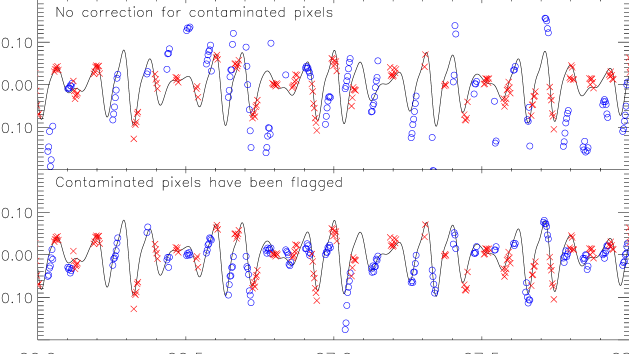
Figure 4: Light curve for SX Phe star V2 in F555W ($\circ$) and F814W ($\times$) when using two different reduction techniques (see text for details). The abscissa is the heliocentric Julian date minus 2451300

3.2 Further analysis

Two other time-series analyses should be mentioned here. Gilliland et al. (gill2000 (2000)) describe use of difference image analyses for obtaining optimal results for the unsaturated stars comprising the primary data use. The difference image analysis provided time-series precisions averaging a factor of two better than those presented here for unsaturated stars, but cannot be applied at all to the saturated stars. A second approach to saturated-star extractions has been developed by one of us (RLG, Gilliland gill94 (1994)) making use of aperture photometry including the saturated pixels. The latter approach provides generally comparable results to those described here for the PC1 extractions.

4 Time-series analysis

To perform the frequency analysis of the light curves we used the software package period98 developed by Sperl (sperl98 (1998)). Figure 5 shows the amplitude spectrum for the SX Phe star V2 (top left plot) and also the resulting amplitude spectra when the variation corresponding to the most significant peaks has been subtracted. The arrows show the frequencies in cycles per day (c/d) — one barely significant peak at 14.88 c/d is labeled “HST”, and may be due to the 96.4 minutes orbital period of the observatory. The dotted line is the empirically determined 4$\sigma$ detection limit; peaks below this are not considered to be significant. All mode frequencies, amplitudes, phases, and errors are quoted in Table 2. We note that the light curves have been analyzed independently by three of the authors using different software — and our results agree.

Figure 5: Amplitude spectra for the SX Phe star V2 computed when using the combined F555W and F814W light curve (top left plot and labeled A). The other three plots (labeled B,C, and D) show the resulting amplitude spectra when the modes marked by arrows have been subtracted. Note that the scales on the ordinate differ. The dotted line is the 4$\sigma$ detection limit

The primary modes of V2 have sufficient amplitude to provide unambiguous detections from both the 1993 (Gilliland et al.  gill98 (1998)) and 1999 time series. We now consider the other four SX Phe stars for which some of the modes claimed previously were near the detection limit provided by the 1993 data. Figure 6 shows the amplitude spectra for V3, V14, V15, and V16 with the original $U$-band (1993) and $I$-band (1999) amplitudes transformed to a common $V$ estimate by scaling by central wavelength ratios. Time series for V3 and V15 are based upon combined $V$ and $I$ (as for V2) data making use of techniques previously described for analyzing saturated stars. For V14 and V16 the stars never saturate in $I$ exposures; for these we use only the 653 unsaturated images and the more precise photometry provided by difference image analyses. Results for V3, V15, and V16 show that all primary modes claimed from the 1993 data are present, and these will be further discussed in Section 5.5. V14 was the least significant detection from the 1993 data, and was only selected (Gilliland et al.  gill98 (1998)) as a likely variable by searching for repeated low amplitude peaks with spacing characteristic of successive radial modes. The 1999 data for V14 clearly show that not even a slight hint of the claimed modes exists; the most likely interpretation is that V14 is not a variable and we will not further consider V14 as an SX Phe star. The V14 amplitude spectrum for 1999 nicely illustrates a characteristic of the extensive $HST$ observations – a very clean spectrum that in fact stays flat from below 1 cycle/day out to the Nyquist frequency of 180 cycles/day. V16 was also only found as a variable from the 1993 data based on a search for successive radial overtone peaks; in this case the 1999 data clearly confirm oscillations are again present.

Figure 6: Amplitude spectra for V3, V14, V15, and V16 are shown comparing the 1993 (Gilliland et al.  gill98 (1998)) results with the new 1999 data. All amplitudes have been scaled as needed by wavelength to provide V-band equivalent magnitudes. Frequency units are cycles per day. All modes claimed from the 1993 data are marked with vertical bars under the corresponding peaks

Table 2: Frequencies, amplitudes, and phases for modes for the observed SX Phe stars. Modes above the 4$\sigma$ level are marked with $*$ while less significant modes are marked with $?$. Numbers in parenthesis are the statistical errors. The frequencies found by Gilliland et al. (gill98 (1998)) are given in the rightmost column. Note that the formal errors on the frequencies of the new results are lower by almost an order of magnitude compared to Gilliland et al. (gill98 (1998)). In column 5 $\nu_{1}$ and $\nu_{2}$ are the frequencies of the primary and the secondary mode

Star Frequency $V$ Amplitude Phase Mode Gilliland et al. [c/d] [mag] [c] combination V2 9.816(0.002) 0.044(0.001) 0.662(0.004) * $\nu_{1}$ 9.807(0.013) 12.684(0.002) 0.034(0.001) 0.488(0.005) * $\nu_{2}$ 12.700(0.016) 22.490(0.005) 0.012(0.001) 0.187(0.014) * $\nu_{1}+\nu_{2}$ 22.494(0.057) 2.866(0.007) 0.011(0.001) 0.620(0.014) * $\nu_{2}-\nu_{1}$ 19.604(0.020) 0.008(0.001) 0.564(0.076) * $2\nu_{1}$ 25.354(0.013) 0.005(0.001) 0.351(0.035) ? $2\nu_{2}$ 6.914(0.013) 0.005(0.001) 0.179(0.025) ? $2\nu_{1}-\nu_{2}$ V3 17.929(0.001) 0.036(0.005) 0.624(0.007) * $\nu_{1}$ 17.948(0.022) 18.359(0.004) 0.009(0.005) 0.925(0.017) ? $\nu_{2}$ 18.585(0.064) V15 30.110(0.004) 0.0084(0.0004) 0.727(0.007) * $\nu_{1}$ 30.157(0.053) 34.807(0.010) 0.0038(0.0004) 0.493(0.016) * $\nu_{2}$ 34.671(0.070) V16 31.988(0.005) 0.0039(0.0005) 0.055(0.016) * $\nu_{1}$ 31.894(0.064) 28.165(0.008) 0.0016(0.0005) 0.256(0.016) ? $\nu_{2}$ 28.116(0.071)

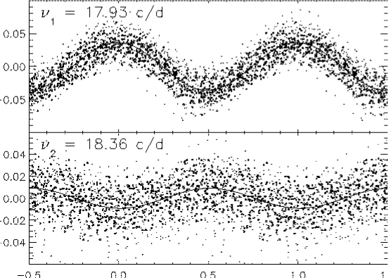
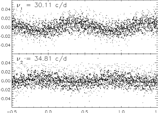
Figure 8: Phase diagram for V3 and V15 for two modes

In Figures 7 and 8 we show the phase diagrams for the three largest amplitude double-mode stars in our sample. In each diagram all known modes have been subtracted except for one mode, the frequency of which is shown in the top left corner. Note the different scale on the ordinates.

4.1 Search for new SX Phe stars

The original HST data (WF/PC; Gilliland et al. gill98 (1998)) used to find SX Phe variables in 47 Tuc covered an area of 66 $\times$ 66 arcsec², with the cluster centre about 10 arcsec from the field of view centre. The new search domain with WFPC2 observing in 1999 is such that the PC1 field of view is almost entirely contained within the original search area, while the much larger field of view of the WF CCDs is (at the 90% level) outside the original search space. We have extracted time series for 2968 saturated stars on the 4 WFPC2 CCDs using the technique of Gilliland (gill94 (1994)). Near the domain in the CMD where the previous SX Phe stars were found the root-mean-square variations in the resulting time series are $\sim$ 1 – 2% (albeit with non-Gaussian characteristics). We note that the previously detected SX Phe variables V2, V3, V15, and V16 are easily observed in these new time series. Although the new survey field of view is much larger than that previously surveyed, it is also on average farther from the cluster center. In the domain $15.0<V<17.0$, $0.2<V-I<0.45$ the original search contained about 25 stars of which 6 are SX Phe variables. The number of new stars surveyed within this box in the CMD is only 7 consistent with the known, strong central concentration of BSS. The time series for all of the newly surveyed BSS were analyzed by taking power spectra and searching for significant peaks; no convincing evidence of variables was found. Amplitudes of 0.01 magnitudes would in general be easily seen unless the period is similar to the 96.4 minute HST orbital period or its harmonics.

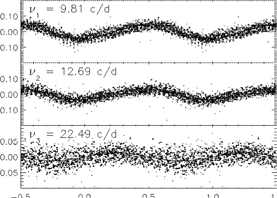
Figure 7: Phase diagrams for V2 for the three main modes

5 Results

5.1 The colour-magnitude diagram

The conversion from the instrumental to standard $V,I$ (Johnson-Cousins) magnitudes was done following the “photometric cookbook” of Holtzman et al. (holtzman (1995)). We correct for geometric distortion and the “34th row effect” (Anderson & King 34throw (1999)). We have corrected for the charge-transfer efficiency (CTE) problem by following the formulation of Stetson (cte-effect (1998)) and we include his new photometric zero-points.

Systematic differences between long and short exposures obtained with the HST have been reported in the literature (see e.g. Kelson et al. longshort (1996)). There is a tendency that measurements of stellar brightness from frames with long exposure times yield brighter magnitudes than short-time exposures. To be able to correct for the “long-short anomaly” we reduced some additional short exposures obtained for our field: Four 1.6 s exposures in F555W and F814W (the same field as the 160 s exposures).

We then determined the offsets in $V$ and $I$ from frames with different exposure times. The offsets are: $\Delta V$(160-1.6s)$=-0.104\pm 0.004$ (1042 stars), and $\Delta I$(160-1.6s)$=-0.0554\pm 0.0035$ (1034 stars). We stress that this is after correcting for the CTE effect, i.e. the long-short anomaly is “real” and not only a part of the CTE problem. A possible explanation for the offsets is the difficulty of determining the $0.5$ arcsec aperture correction due to crowding. This correction is needed when following the calibration “cookbook” of Holtzman et al. (holtzman (1995)).

After the removal of the offsets we compare our CMD with several results from the literature. We have found the average $V$ of the stars in the transition between the turn-off and the red giant branch: $V_{\rm TO/RGB}=17.31$ near $V-I=0.80$. The mean of Hesser et al. (hesser (1987)), Kaluzny et al. (kaluzny (1998)), and Alcaino & Liller (alcaino (1987)) is $V_{\rm TO/RGB}=17.18\pm 0.04$. We thus apply an offset of $\Delta V=17.18-17.31=-0.13$. The offset in $I$ is found from the colour of the turn-off. The mean colour from Kaluzny et al. (kaluzny (1998)) and Alcaino & Liller (alcaino (1987)) is $(V-I)_{\rm TO}=0.695\pm 0.02$. We find $\Delta I=-0.096$.

The final colour-magnitude diagram (CMD) is shown in Figure 9 where the BSS stars have been marked. The parameters of the SX Phe stars are given in Table 3.

Two groups in our team have performed the standard photometry in order to detect systematic differences. The first group reduced each short exposure image individually while the second group worked on combined images. The photometry of the SX Phe stars and the CMD presented here are the results of the first group — here we mention the main differences. After correcting for the offsets mentioned above (TO/RGB transition level and colour of the turn-off) the results from both groups based on the short exposures generally agree: We note that for the CMD presented here, the brightest part ($V<14.5$) of the giant branch is more red ($\Delta(V-I)=0.10$) than the ground-based study by Da Costa & Armandroff (redbranch (1990)). Our second group finds $\Delta(V-I)=-0.05$ for these stars. In the interesting case of the SX Phe star V2 both groups agree that $V=15.07\pm 0.02$ while we find discrepant results for the red filter: $I=14.63\pm 0.03$ and $I=14.80\pm 0.03$. The most immediate explanations for this are the crowding around V2 (cf. Figure 1) and that the images are under-sampled. We note that systematic errors of the order 0.03 magnitudes may still be present (see e.g. Stetson cte-effect (1998)) for all stars.

To transform the empirical data into the theoretical plane we adopted the bolometric corrections (BCs) and the colour-temperature relations provided by Bessell, Castelli, & Plez (1998). By means of a linear interpolation of the tables for ${\rm[Fe/H]}=-0.5$ and $-1.0$ we estimated a new list of BCs for ${\rm[Fe/H]}=-0.83$. For MS stars we use $\log g=4.5$, while for BSS we use $\log g=4.0$. As a special case we assumed $\log g=3.7$ for V2, since this SX Phe has already evolved off the MS. Note that such a value is somewhat lower than the value obtained on the basis of an evolutionary track with $M/M_{\odot}=1.5$ (VandenBerg, private communication). On the basis of these assumptions and of the observed colour (two independent determinations) we find that the effective temperature for V2 ranges from $T_{\rm eff}=7100$ K ($(V-I)_{0}=0.39$) to $T_{\rm eff}=7700$ K($(V-I)_{0}=0.23$). We have used $T_{\rm eff}=7100$ K for V2 and find BC $=-0.02$ mag. The BCs for all stars were estimated by adopting a similar procedure. The BC for the SX Phe stars are listed in Table 3.

The distance modulus of 47 Tuc has been determined several times in the literature. VandenBerg (vandenberg2000 (2000)) found $(m-M)_{V}=13.37\pm 0.05$ (using new isochrones and $B,V$ photometry by Hesser et al. hesser (1987)). Grundahl et al. (grundahl (2001)) made Strömgren photometry on 47 Tuc and 14 field sub dwarfs. By fitting the lower main sequence of 47 Tuc to the field stars they find a distance modulus $(m-M)_{V}=13.32\pm 0.04$. The quoted errors ignore systematic errors, e.g. the zero point of the metallicity scale and the error on the interstellar reddening. The systematic error is of the order 0.10 magnitudes. These three independent studies all seem to deviate significantly from Carretta et al. (hipparcos-dm (2000)) and Salaris & Weiss (salaris (1998)) who find $(m-M)_{V}=13.55\pm 0.09$ and $13.50\pm 0.05$, respectively. We finally draw attention to the study of the white dwarf cooling sequence by Zoccali et al. (zoccali99 (1999)). They find a distance modulus of $(m-M)_{V}=13.15\pm 0.12$ (assuming again $E(B-V)=0.032$). In the following, we adopt the value obtained by VandenBerg (vandenberg2000 (2000)), i.e. $(m-M)_{V}=13.37\pm 0.05$.

5.2 The Hertzsprung-Russell diagram

Figure 10 is the Hertzsprung-Russell (HR) diagram for 47 Tuc in which all BSS stars and main-sequence stars with the best photometry are shown. The five known SX Phe stars have been labelled. Also seen in the plot are evolutionary tracks for models computed with the evolution code by Christensen-Dalsgaard (Petersen & Christensen-Dalsgaard otzen96 (1996, 1999)). The abundances of hydrogen, helium, and heavy elements are $(X,Y,Z)=(0.754,0.241,0.005)$ which is appropriate for 47 Tuc according to VandenBerg (vandenberg2000 (2000)).

We note that Salaris & Weiss (salaris (1998)) discuss the evidence for a somewhat higher value of $Y=0.273$ for 47 Tuc. For example they use the $R$-method (Buzzoni et al. buzzoni (1983)) with $R=1.75\pm 0.21$ and $1.86\pm 0.36$ based on Buzzoni et al. (buzzoni (1983)) and Hesser et al. (hesser (1987)), respectively. This corresponds to a mean $Y=0.28\pm 0.04$ which is roughly consistent with the value we have adopted (using the calibration by Buzzoni et al. buzzoni (1983)). We note that a more recent determination of the $R$ parameter was done by Zoccali et al. (zoccali00 (2000)) based on observations with HST. They find $R=1.52\pm 0.13$ corresponding to $Y=0.246\pm 0.012$ (again using Buzzoni et al. buzzoni (1983)). Based on this short discussion we have adopted the same helium content as VandenBerg (vandenberg2000 (2000)), i.e. $Y=0.241$.

The age of the cluster was determined to be 11.5 Gyr by VandenBerg (vandenberg2000 (2000)) from the $B,V$ photometry by Hesser et al. (hesser (1987)). The new combined $V,I$ photometry from HST indicates that this age estimate may be a bit too young. In Figure 10 we have also shown an isochrone of age 12.5 Gyr computed by VandenBerg (private communication). For comparison the $0.9\,M_{\odot}$ evolutionary model in Figure 10 reaches the turn-off at $\log T_{\rm eff}=3.78$ after $\approx 10$ Gyr and starts climbing the Hayashi-track around $\approx 13$ Gyr: This evolutionary model is indeed comparable with stars near the observed turn-off. Thus our models are in qualitative agreement with VandenBerg. We note that Salaris & Weiss (salaris (1998)) find an age of $(9.2\pm 1.0)$ Gyr for 47 Tuc.

The BSS population is clearly seen in the HR diagram in Figure 10. The “life span” for models with the metallicity of 47 Tuc and masses $1.4\,M_{\odot}$ and $1.6\,M_{\odot}$ (typical for BSS stars) is only about 1.8 Gyr and 1.3 Gyr, respectively (the time to reach the hook). Thus it is evident that these stars have formed late in the evolution of the cluster, probably by a merger or collision between two stars of mass below the turn-off mass.

The observed instability strip for population I $\delta$ Scuti stars is also shown in Figure 10 (Breger instab-strip (1990)). Four of five SX Phe stars are located inside the instability region. Even when taking into account the uncertainty of the temperature V14 is not inside the instability region — possibly explaining the lack of variation for this BSS (cf. the amplitude diagram in Figure 6).

Figure 9: Combined CMD for 47 Tuc. Filled dots mark the BSS stars, and the SX Phe stars have been labeled

Detailed modelling of the BSS stars is hampered by the uncertainties relating to their formation (e.g. Benz & Hills bss-merginge (1987), bss-merging (1992); Bailyn & Pinsonneault bss-collision (1995)). This likely leads to changes in composition due to mixing; in the extreme case where stars at the turn-off are completely mixed, the resulting homogeneous helium content would be $Y\approx 0.34$. Furthermore, it is plausible that, for example, the orbital angular momentum in a merging binary star would lead to a very rapidly rotating BSS. A detailed investigation of such effects is beyond the scope of the present paper. However, we have explored the effects of a change in the composition: In addition to the models with the standard helium abundance (SHe, $Y=0.241$), we have considered models with increased helium content (IHe, $Y=0.261$) and masses $1.40\,M_{\odot}$ and $1.50\,M_{\odot}$; these are also shown in Figure 10 (dashed lines).

From the evolutionary tracks it is possible to estimate the masses of the SX Phe stars. A unique case is V2 for which an unambiguous estimate can be given: The evolutionary tracks are almost horizontal around V2, hence the uncertainty in $T_{\rm eff}$ is not so important for the mass estimation from the position in the HR diagram. For V2 we find $M_{\rm HR}/M_{\odot}\simeq 1.54\pm 0.05$ for the standard helium abundance; using instead the models with increased helium abundance (IHe) we obtain $M_{\rm HR}/M_{\odot}=1.50\pm 0.05$. The other SX Phe stars all lie around the hooks of the evolutionary tracks and the mass estimate is more uncertain for these stars ($\pm 0.10\,M_{\odot}$). In Table 3 we have given mass estimates and various parameters of the SX Phe stars.

In Figure 10 the model ages in Gyr are given at three points along the $1.5\,M_{\odot}$ track which is below V2 (in square brackets). Consequently the age of V2 must be somewhat lower than the $\approx 1.9$ Gyr found from this track. If we assume that V2 is following the evolutionary track of a standard model (ignoring formation history, e.g. mixing of the merging stars) and that the position in the HR diagram is correct we can conclude (from an evolutionary track of mass $1.54M_{\odot}$): The age of V2 is around $(1.7\pm 0.2)$ Gyr, $L/L_{\odot}=17.0\pm 0.5$, core burning of hydrogen has ceased $(X_{\rm core}=0)$, and the star has only a few hundred million years left before it will start climbing the Hayashi track and eventually go into the helium-burning phase.

Table 3: Fundamental parameters for the observed SX Phe stars. Typical errors are $(0.03,0.04,0.14,0.02,200$ K$)$ for $(V,V-I,M_{\rm bol},{\rm BC}_{V},T_{\rm eff})$. For the mass in column 6 the error estimate is $\pm 0.05\,M_{\odot}$ for V2 and $\pm 0.10\,M_{\odot}$ for the other variables

Star	$V$	$V-I$	$M_{\rm bol}$	${\rm BC}_{V}$	$T_{\rm eff}$	$M/M_{\odot}$
V2	15.07	0.43	1.68	-0.02	7100	1.54
V3	15.93	0.38	2.54	-0.02	7300	1.35
V15	15.28	0.24	1.91	-0.01	7900	1.65
V16	15.76	0.38	2.37	-0.02	7300	1.35

5.3 Double-mode SX Phe stars

For some double-mode SX Phe stars a safe mode identification is possible. Most double-mode pulsators oscillate in radial modes ($l=0$) of low radial order ($n=1-6$). One can put constraints on the astrophysical properties (mass, helium content) of these stars by comparing observed and theoretical data in a period-ratio versus period diagram, the so-called Petersen diagram. In the following we look more closely at the double-mode SX Phe star V2, and then discuss the more difficult stars V3, V15, and V16.

5.4 The double-mode SX Phe star V2

We interpret the dominant observed modes as the the fundamental mode and the first overtone and obtain a period ratio of $\Pi_{1}/\Pi_{0}=0.7739\pm 0.0002$. Gilliland et al. (gill98 (1998)) found $\Pi_{1}/\Pi_{0}=0.7722\pm 0.0014$, i.e. the results are essentially consistent. With the more accurate period ratio obtained from the new longer time series we can constrain the mass of V2 to within a formal error of $0.03\,M_{\odot}$ at a given composition from the position in the Petersen diagram. The error in the mass estimate will be discussed further below.

We have used a series of pulsation models which are extracted from the grid of evolutionary tracks in Figure 10. From the HR diagram we make a rough estimate of the range of stellar masses that are relevant ($1.8>M/M_{\odot}>1.3$). As before, in addition to the standard models we have also calculated pulsation models with higher helium content.

Figure 10: HR diagram of 47 Tuc. Several theoretical evolutionary tracks are shown. For models in the mass interval $M/M_{\odot}=0.9$ to $1.9$ and standard chemical composition tracks are plotted with either solid or dotted lines. Two tracks with increased helium content are also shown with dashed lines. For the $1.5M_{\odot}$ model the age in Gyr is indicated at three points. The filled circles mark the BSS stars and the SX Phe stars have been labeled. The turn-off region can be seen in the lower right corner. The age of the isochrone is 12.5 Gyr (computed by VandenBerg, private communication)

Figure 11 compares the observed period ratio of V2 with data for several stellar oscillation models. Solid lines are computed from models with standard helium abundance (SHe, $Y=0.241$), dashed lines have increased helium content (IHe, $Y=0.261$). A decrease in effective temperature causes an increase in the pulsation period and as a consequence a stellar model moves from left to right in Figure 11 during its post-main-sequence evolution.

Figure 11: The Petersen diagram for several stellar model series. The helium content of the different model series is explained in the top left corner; as indicated, the SHe models cover the mass range $M/M_{\odot}=1.3-1.8$, while IHe models are shown for $M/M_{\odot}=1.4$ and 1.5. In the inserted plot the ages of models with $Y=0.241$ and mass $M/M_{\odot}=1.5$ and 1.6 are given in Gyr

The double-mode SX Phe star V2 is shown in the plot. We estimate the mass of V2 to be $(1.53\pm 0.03)\,M_{\odot}$ for SHe. From the models with IHe we infer the mass to be $(1.45\pm 0.03)\,M_{\odot}$.

The good accuracy of the observed period ratio for V2 — the error bars can be seen in the inserted plot — is due to the long time series with good sampling. In comparison the result by Gilliland et al. (gill98 (1998)) is $\left(1.4^{+0.25}_{-0.15}\right)\,M_{\odot}$ (cf. their Figure 22).

The mass determination is obviously also sensitive to errors in the stellar modelling used in computing periods and period ratios. We have estimated the intrinsic errors arising from numerical effects in the computation of the evolutionary models and their oscillation frequencies; the effect on the computed period ratio $\Pi_{1}/\Pi_{0}$ is minute, less than $10^{-4}$. On the other hand, major contributions to the uncertainty in the mass determination arise from uncertainties in the composition parameters and possible effects from rotation of V2. The possible effects on the helium abundance of mixing associated with the formation of BSS have already been mentioned. To this must be added the uncertainties in the determination of the overall composition of the cluster. Also, it is well known that rotation affects the evolution of stellar models and the derived oscillation frequencies (e.g. Pamyatnykh 2000, Goupil et al. 2000). Fast rotation modifies the evolutionary tracks in the HR and Petersen diagrams, particularly in the post-main-sequence stages where V2 is located. Although the frequency corrections are expected to be relatively small for radial modes, they may be significant. For the high-amplitude $\delta$ Scuti stars (with amplitude $A_{V}>0.3$ mag) rotation is usually slow. However, V2 has relatively low amplitude ($A_{V}=0.15$) and its rotational velocity ($v\sin i$) is not known. Finally, we recall from Section 5.1 that basic parameters of the star, i.e. the effective temperature and the distance modulus, are subject to substantial uncertainty.

Given these uncertainties, to what extent can we trust our mass determinations? A very significant aspect in the interpretation is the consistency between different determinations. As an example, consider the effects of the helium abundance, exemplified by the SHe and IHe model series. From the analysis of the HR diagram (Figure 10) V2 has evolutionary mass $M_{\rm HR}\simeq(1.54\pm 0.05)\,M_{\odot}$ with SHe, for which the period-ratio mass is $(1.53\pm 0.03)M_{\odot}$; for IHe the corresponding values are $M_{\rm HR}\simeq(1.50\pm 0.05)\,M_{\odot}$ and $(1.45\pm 0.03)M_{\odot}$ from the period ratio. Thus for both compositions the two mass determinations agree within the formal error bars, although the match is somewhat better for SHe. We also note that the mass estimates allow a better constraint on the change in the helium abundance resulting from complete mixing. Assuming that the progenitor stars had masses of around $0.75M_{\odot}$ and had evolved for 10 Gyr before the merger, the average helium abundance would be increased by around 0.04 relative to the original value, i.e. twice the difference between SHe and IHe. Since complete mixing is thought to be unlikely during BSS formation, the SHe abundance solution is favoured ($Y=0.241$).

We have adopted a metal content $Z=0.005$ for the models. However, the value of ${\rm[Fe/H]}=-0.83$ from Table 1 with the original definition ${\rm[Fe/H]}=\log(Z/Z_{\odot})$ and $Z_{\odot}=0.019$ gives $Z=0.0028$, and Salaris & Weiss (1998) use $Z=0.008$, since they account for $\alpha$-element enhancement. In addition to the analysis based on standard stellar model series with $Z=0.005$, we have also performed mass estimations using the composition used by Salaris & Weiss (salaris (1998)), i.e. $Y=0.273,Z=0.008$. We find that for this composition we cannot obtain consistent modelling satisfying the observational constraints: V2 fits an evolutionary track in the HR diagram of mass $1.56\,M_{\odot}$ and the period ratio yields the mass $1.67\,M_{\odot}$.

Table 4: Mass determination of the SX Phe star V2 from its position in the HR diagram and from comparison of observed modes with pulsation models. The results when using different chemical compositions are given (see text for details)

Composition	SHe	IHe	S-W
$Y$	0.241	0.261	0.273
$Z$	0.005	0.005	0.008
Method	Mass estimates ($M/M_{\odot}$)
HR-diagram	1.54	1.50	1.56
Pulsation modes	1.53	1.45	1.67

From the period and period ratio we may also infer the age and effective temperature of V2. For the SHe models of mass $1.6$ and $1.5\,M_{\odot}$ we have indicated the age of the models in Gyr in the inserted plot in Figure 11; this can be compared with the ages in the HR diagram in Figure 10 for the $1.5M_{\odot}$ model. The analysis indicates that $T_{\rm eff}$ may be somewhat higher than inferred from our adopted $V-I$ photometry: From the Petersen diagram we infer that $T_{\rm eff}=(7400\pm 150)$ K. The ages roughly agree with Figure 10 when taking the error on $T_{\rm eff}$ into account, leading to an age of $(1.7\pm 0.1)$ Gyr.

The determination of $M_{\rm HR}$ is sensitive to errors in the distance modulus.. An independent estimate of this may be obtained from the period-luminosity-colour-metallicity (PLCZ) relation for SX Phe stars, derived by Petersen & Christensen-Dalsgaard (otzen99 (1999)) from theoretical stellar models. This relation is sensitive to the adopted values of $Z$ and in particular of $T_{\rm eff}$. In the above analysis of V2 we have considered the $T_{\rm eff}$-interval $7100$ to $7700$ K. For the preferred $Z=0.005$ the PLCZ relation gives the corresponding interval in $M_{\rm bol}$ of 1.98 to 1.56 mag. We note that this is in rough agreement with the value given in Table 3 for V2 ($M_{\rm bol}$ = 1.68) and hence justifies our use of the VandenBerg (vandenberg2000 (2000)) distance modulus. Although this is somewhat speculative, a higher temperature for V2, as inferred from the period, seems to be necessary to explain the distance modulus inferred from the main period. We recall from Section 5.1 that independent estimates of $V-I$ gave discrepant results for V2.

We thus have two clues that indicate the $T_{\rm eff}$ of V2 may be higher than what we find from the colour (i.e. $V-I=0.43$ or $T_{\rm eff}=7100$ K): 1) A comparison of the theoretical model ages that best fit the position in the Petersen diagram and the HR diagram do not agree. 2) The PLCZ calibration from Petersen & Christensen-Dalsgaard (otzen99 (1999)) gives a small distance modulus ($(m-M)_{V}=13.1\pm 0.1$) for $Z=0.005$ and $T_{\rm eff}=7100$ K. Both these observations indicate a higher value of $T_{\rm eff}$. If for V2 we assume $T_{\rm eff}=(7500\pm 200)$ K appropriate to the independent $V-I$ = 0.27 determination we find that the PLCZ relation gives a distance modulus of $(m-M)_{V}=13.4\pm 0.1$ in agreement with VandenBerg (vandenberg2000 (2000)) and Grundahl et al. (grundahl (2001)) — and with this temperature the new position of V2 in the HR diagram agrees with the position in the Petersen diagram within error-bars.

It is evident that there are a number of uncertainties concerning the parameters and modelling of V2. Also, we have not been able to take into account the possible effects of rotation on the inferences. However, the fact that we obtain a consistent description of V2 using standard modelling without rotation — which is the simplest possibility — gives us some confidence in this modelling. Since V2 is a relatively evolved and hence old BSS at $\sim$1.7 Gyr it could by now have lost significant angular momentum even if it was formed initially as a rapid rotator. Thus, from this discussion we maintain that a reasonable estimate for the mass of V2 is $M/M_{\odot}=1.54\pm 0.05$; we stress, however, that this assumes V2 to have the same chemical composition as an average star in the cluster.

In Table 4 we present the results of the mass estimation of V2 for the three different chemical compositions discussed above.

We finally note that we have also found new low-amplitude modes for V2 (see Table 2), but their frequencies are simply linear combinations of the frequencies of the two main modes. This indicates that the modes are interacting non-linearly as was also noted by Gilliland et al. (gill98 (1998)), and the pattern given in Table 2 is in perfect agreement with predictions from Garrido and Rodriguez (1996).

5.5 V3, V15, and V16

The interpretation of the modes of V3 is difficult since the period ratio is close to unity. Gilliland et al. (gill98 (1998)) propose that it is a rotationally split non-radial mode ($l=1$). If this is true the rotational period of V3 (based on the splitting in Table 2) is $P_{\rm rot}=(2.33\pm 0.03)$ days. Gilliland et al. (gill98 (1998)) found a significantly faster rotation period $P_{\rm rot}=(1.65\pm 0.2)$ days.

The interpretation of the double-mode SX Phe star V15 is also difficult. If this star is assumed to be a “classical” double-mode pulsator oscillating in radial modes, it must be oscillating in high overtones. The observed period ratio is $\Pi_{N}/\Pi_{n}=0.8651\pm 0.0003$ which is below the ratio calculated from theoretical models with radial orders 5 and 6 — but above the calculated ratio for radial orders 4 and 5. Figure 12 shows several series of models oscillating in these high overtones. The 10$\sigma$ error bars are shown.

The result for V15 by Gilliland et al. (gill98 (1998)) was $\Pi_{N}/\Pi_{n}=0.8698\pm 0.0023$. This result was consistent with V15 oscillating in two high overtones with their analysis, i.e. orders 4 and 5. With the new results none of the calculated models fits the observed properties of V15. This is also the case when using the composition from Salaris & Weiss (salaris (1998)), i.e. models with higher helium and heavy element content.

Possible explanations for the apparent discrepancy are e.g. (i) that at least one of the observed modes is a non-radial mode, or (ii) that the frequencies are modified by rotation of the star. A clear interpretation of the modes in V15 cannot yet be made.

We note that for the two modes in V15 the periods determined from 1993 and 1999 observations agree to 0.8$\sigma$ and 2.0$\sigma$ for the large- and small-amplitude peaks, respectively. Either spurious agreement with radial overtone period ratios was allowed by the larger errors in the results of Gilliland et al. (gill98 (1998)), or the lower-amplitude peak represents different modes having been excited 6 years apart.

Interpretation of the double-mode star V16 is also problematic here. The mode near 32 cycles/day from 1993 is clearly present in the 1999 observations with the new frequency 1.2$\sigma$ from the original value. The mode near 28 cycles/day is at a lower amplitude in 1999 and at marginal $\sim$3$\sigma$ significance in each epoch separately. Taking the agreement (to 0.8$\sigma$ from the 1999 period) as confirmation of this mode and evaluating the period ratio yields $\Pi_{N}/\Pi_{n}=0.8805\pm 0.0002$ (compared to 1993 data result of 0.8816 $\pm$ 0.0028) which falls just above the period ratios for orders 5 and 6 in Figure 12. However, there are evidently other modes present to equal or higher significance – these cannot all be radial modes. The significance of amplitudes quoted in Table 2 represent very conservative values based upon establishing a local mean in the amplitude spectra and considering the ratio of the mode amplitude to this. Since our power spectra for non-variable stars remain flat consistent with white noise, it may well be appropriate to base the errors on means over the full available frequency range. As an example, for V16 adopting a global normalization for the amplitude spectrum noise would increase the significance of the three modes near 28, 29, and 31 cycles/day to over 8$\sigma$ each with the possibility that yet weaker modes are also present.

Figure 12: Petersen diagram showing radial overtones of orders four to six for several stellar model series. The $\bullet$ mark the SX Phe stars V15 and V16. The vertical bars are the 10$\sigma$ error on the period ratio

5.6 Future work

How can the analysis of the SX Phe variables in 47 Tuc be improved in the future? From the discussion above it is evident that accurate determinations of effective temperatures will give stronger constraints on the modelling. Secure determinations of the chemical composition and studies of rotation will also be important.

A more ambitious project is simultaneous modelling of several SX Phe variables in 47 Tuc following the philosophy of the programme for asteroseismology in open clusters (e.g. Frandsen et al. 1996). The new results for V15 and V16 are consistent with the presence of some non-radial modes, perhaps with high overtone radial modes present as well. Another challenging case is V1, which Gilliland et al. (gill98 (1998)) found to be a triple-mode variable with period ratios that cannot be explained by radial oscillations of standard evolutionary models with the accepted composition of 47 Tuc. Either this star, with an amplitude of about 0.15 mag, has a low $Z\approx 0.001$, its modes are non-radial or perhaps a large effect from rotation needs to be considered. It seems clear that more detailed studies of the SX Phe stars in 47 Tuc will provide valuable asteroseismological information.

6 Conclusions

The unique time series of 8.3 days from HST of 47 Tuc analyzed here was optimized to look for planets around stars fainter than the turn-off. We have shown that it is possible to obtain good photometry for the saturated stars by identifying and flagging (i.e. not using) pixels that are contaminated by neighbouring pixels due to bleeding signal. We have thus extracted good (1-3% noise) light curves for the saturated stars. No new variable BSS stars were found in the sample but have analyzed five of the six known SX Phe stars in the core of 47 Tuc (V1 was not in the field of view). For V14 we do not detect the oscillation signal that has been claimed previously. For three of the double-mode stars (V2, V15, and V16) we have used theoretical stellar models to attempt to determine their masses: Both through the position in the HR diagram (using the observed magnitudes) and in the Petersen diagram (using the observed periods).

The most striking result from this study is the determination of the mass of the SX Phe star V2. From the HR diagram (not depending on the uncertainty of $T_{\rm eff}$) and the Petersen diagram we infer a mass of $M_{\rm V2}=(1.54\pm 0.05)\,M_{\odot}$. Important sources of error in this mass estimate of V2 are the chemical composition and effects of rotation; even so, we believe that we have obtained the so far most precise determination of the mass of a BSS (see Shara et al. shara (1997)). Further progress requires a spectroscopic study to constrain $T_{\rm eff}$, rotational velocity, and chemical composition for V2; this would be difficult from the ground due to crowding, but it is feasible with HST. Our results indicate that, with such additional data, we would be able to obtain strong constraints on the processes that lead to the formation of BSS.