The properties of field elliptical galaxies at intermediate redshift. II: photometry and spectroscopy of an HST selected sample

Abstract

A sample of field early-type galaxies (E/S0) at intermediate redshift ($z\sim 0.1-0.6$) is selected, based on morphology and colours from HST-WFPC2 parallel images. Photometric structural parameters (effective radius $R_{\textrm{e}}$ and effective surface brightness $SB_{\textrm{e}}$) are derived through the F606W and F814W filters, using luminosity profile fitting and two-dimensional fitting techniques. The combined parameter that enters the Fundamental Plane ($\log R_{\textrm{e}}-\beta SB_{\textrm{e}}$, with $\beta\approx 0.32$) is shown to suffer from significantly smaller uncertainties (r.m.s. 0.03) than the individual structural parameters (e.g. $\sim 15$ per cent r.m.s. on the effective radius).

High signal-to-noise intermediate resolution spectra, taken at the ESO-3.6m, yield redshifts for 35 galaxies and central velocity dispersions for 22 galaxies. Central velocity dispersions are derived using a library of stellar templates covering a wide range of spectral types, in order to study the effects of templates mismatches. The average random error on the central velocity dispersion is found to be 8 per cent and the average systematic error due to template mismatch is found to be 5 per cent. The errors on velocity dispersion measurement and the effects of template mismatches are studied by means of extensive Montecarlo simulations. In addition, we investigate whether the determination of the velocity dispersion is sensitive to the spectral range used, finding that the value of velocity dispersion is unchanged when the spectral regions that include the absorption features Ca HK and NaD are masked out during the fit.

1 Introduction

This paper is the second of a series devoted to the investigation of the internal and structural properties of field early-type galaxies (E/S0) at intermediate redshift ($0.1<z<1$), and of the properties of their stellar populations. In particular, the aim of this series of papers is to investigate how empirical scaling laws such as the Fundamental Plane (FP; Djorgovski & Davis 1987; Dressler et al. 1987) and the Kormendy (1977) relation evolve with redshift. These studies are complemented with the measurement of metallicity and age of stellar populations by means of the Lick/IDS absorption lines indeces (Trager et al. 1998).

For this project we have collected high signal-to-noise (S/N) spectra at intermediate resolution (resolving power $\lambda/\Delta\lambda\sim 1000$, where $\Delta\lambda$ is the full width half maximum resolution) for a well-defined sample of field early-type galaxies in the redshift range $z\approx 0.1-0.6$. The sample is selected from images obtained with the Wide Field and Planetary Camera 2 (WFPC2) on board the Hubble Space Telescope (HST) taken from the HST-Archive.

The motivations of the project and the first results of this study have been discussed discussed in the paper presenting the analysis of the pilot sample (Treu et al. 1999; hereafter T99). In this paper, we describe in detail the selection of a larger sample of 35 objects, and we present the surface photometry and the kinematic spectroscopic measurements. An extended discussion of the state of the art in this research area and of the objectives of our work is given in a companion paper (Treu et al. 2001, submitted to MNRAS; hereafter PIII), where the evolution of the Fundamental Plane and Kormendy relation is analyzed.

This paper is organized as follows. The sample selection criteria and the characteristics of the sample are discussed in Section 2. In Section 3, we report on the measurement of the photometric parameters. The measurement of redshifts and central velocity dispersions is described in Section 4. The caveats of the photometric and kinematic measurements are extensively discussed. In particular, we discuss: i) the accuracy that can be achieved in measuring the combination of photometric observables that enters the Fundamental Plane; ii) the effects of resolution on the measurement of internal velocity dispersion, by means of Montecarlo simulations; iii) the stability of the measured internal velocity dispersion with respect to the rest frame spectral region used for the fit. A summary is given in Section 5.

The Hubble constant is assumed to be H${}_{0}=50h_{50}$km $\textrm{s}^{-1}$Mpc^-1. The matter density of the Universe and the cosmological constant in dimesionless form are indicated as $\Omega$ an $\Omega_{\Lambda}$ respectively.

2 Sample selection

2.1 Selection criteria

The targets used in this study have been chosen from a sample of random early-type galaxies (E/S0) found in the WFPC2 parallel images collected by the Medium Deep Survey (Griffiths et al. 1994). The Medium Deep Survey consists of a database of 250 WFPC2 fields with at least 1 image in each of the filters F606W and F814W, which broadly correspond to Johnson-Cousins filters V and I; we refer to these filters as V₆₀₆  and I₈₁₄. The images have been reduced and analyzed by the MDS group and the complete catalog is available to the scientific community (Ratnatunga, Griffiths & Ostrander 1999).

For the sample selection we used the following criteria:

1. Morphology clearly defined as early-type. We selected the galaxies classified by the MDS as pure bulges or disc plus bulge objects with bulge-to-total luminosity (B/T) greater than 0.3 (the MDS group considers $r^{1/4}\,$  and exponential luminosity profiles, indicating them as bulge and disc luminosity profile respectively; see the MDS publications for details). All galaxies were inspected by eye to check their morphology and some of them were rejected as mis-identifications (stars or galaxies with clearly present spiral structure). We did not exclude from the sample galaxies with nearby companions or disturbed galaxies, in order not to bias against merging and interaction.

2. Sufficiently high luminosity: (I₈₁₄ $<19.3$), which is the effective limit with EFOSC2 at the ESO-3.6m with the adopted grism #9 in normally good seeing conditions ($0\aas@@fstack{\prime\prime}8-1^{\prime\prime}$).

3. High galactic latitude: ($|b|>15^{\circ}$), to limit foreground star contamination and galactic extinction.

4. Low extinction: ($\textrm{E(B-V)}<0.2$), as measured by Schlegel, Finkbeiner & Davis (1998), to reduce the possibility of photometric errors due to patchy reddening.

5. Appropriate colour: ($0.95<$ V₆₀₆-I₈₁₄ $<1.7$), which is the entire range spanned by E/S0 in the approximate redshift range $z=0.1-0.6$.

6. Clustering properties. Parallel images are taken at random pointings within a few arcminutes of the primary target. Therefore, when the primary target is a known cluster, the parallel image can also contain part of the cluster. In order to avoid such contamination, and to obtain an unbiased field sample, images centred on known clusters were discarded from the analysis.

2.2 Discussion of the adopted selection criteria

Apart from the natural requirements on the magnitude limit and the limits on galactic latitude and foreground extinction, some selection criteria deserve a thorough discussion. In fact, understanding the selection criteria is a crucial step for a meaningful interpretation of the data (e.g., see the discussion in Schade et al. 1999 on morphology and colour selection criteria).

Morphological Selection. We checked our morphological selection criterion (B/T $>0.3$) by studying the distribution of B/T values for the galaxies morphologically classified as early-type by Abraham et al. (1996). By matching absolute coordinates, we cross-correlated the MDS and Abraham et al. catalogs down to I₈₁₄ $=21$ recovering the B/T value assigned by the MDS to each galaxy visually classified as an early-type by Abraham et al. (1996). The distribution of B/T values found by the MDS group is plotted in Figure 1. We conclude that our threshold in B/T does not exclude a priori any significant part of the early-type galaxy population.

Colour selection. Our experimental setup was tuned to work in the redshift range $z=0.1-0.6$. Therefore, we chose very loose colour cuts that at the same time could reject E/S0 outside our target redshift range ($z<0.1$ or $z>0.6$) and include the widest range of stellar population properties. The colour-redshift relation for our sample is shown in Figure 2. It is noticed that at any given redshift there are objects with early-type morphology that are significantly bluer than the reddest ones. The effect of the adopted colour selection criterion on the study of the evolution of stellar populations is discussed in PIII.

Clustering Properties. We did not attempt to identify and to exclude members of groups or poor clusters. In fact, four of the six objects for which we have obtained FP parameters in T99 are likely to be members of a group (or a poor cluster). Hence, the early-type galaxies in our sample should be representative of a random pointing, magnitude-selected, sample of objects.

Figure 1: Comparison between the morphological classification of Abraham et al. (1996) and our selection criteria. The catalog of all galaxies visually classified as E/S0 by Abraham et al. (1996) was correlated with the MDS catalog by matching the absolute coordinates. The distribution of the bulge-to-total luminosity ratio (B/T) measured by the MDS for this catalog is plotted. A small value of the B/T cut (we adopted B/T$>0.3$) is needed in order not to reject a significant number of early-type galaxies.

Figure 2: Observed V₆₀₆-I₈₁₄  colour (corrected for foreground extinction) as a function of redshift for our sample. The galaxies are plotted as pentagons (E), squares (E/S0) or triangles (S0) according to their morphological classification. Morphological classification based on HST morphology and surface photometry is discussed in Section 3.4. Peculiar galaxies are identified by an open symbol. In order of increasing redshift they are: F3 ($z=0.222$; central dust lane, see Section 3), E2, C2 ($z=0.398,0.425$ strong emission lines; see the spectrum of E2 in Figure 8), and B3 ($z=0.490$; strong Balmer absorption features, see Figure 8). Note that at any given redshift morphologically classified objects span a significant range in colour.

2.3 The sample

We took spectra of 25 galaxies satisfying the adopted colour and magnitude selection criteria. For 22 of them the signal-to-noise ratio achieved is sufficient to measure accurate velocity dispersions (see Section 4). By rotating the slit on the sky, we observed spectra for 10 additional early-type galaxies as secondary targets. For 6 secondary early-type galaxies the signal-to-noise ratio achieved is sufficient to measure velocity dispersions. The redshift has been measured for all the 35 galaxies for which we present photometry.

In Section 4, where we are mostly interested in discussing the measurement of velocity dispersions, we will consider all the galaxies including the secondary targets. In turn, when analyzing the results of this study in terms of evolution of the stellar populations of E/S0 (as in PIII), we will consider only the galaxies satisfying the adopted selection criteria.

Table 1 lists the observed objects (the digit in the adopted name indicates the observing run when the spectra were taken, see Section 4) with their coordinates and MDS identification. The objects are flagged to indicate whether they satisfy all the selection criteria (sel=2), all criteria except that they are fainter than the limit I₈₁₄ $=19.3$ (sel=1), or they are added only as the best secondary target in the field (sel=0). For some of the objects the MDS photometry was not available (galaxy D3 is not considered by the MDS group because it is close to the edge of the combined frame used, see Table 2; sel=nn), or was not reliable (chip edge for galaxy Q3, dust lane for galaxy F3; sel=-1). For easy reference Table 1 also lists for each object the number of spectroscopic observations, the total spectroscopic integration times, the S/N achieved, and the redshift of the object.

Table 1: Galaxy identification. For each galaxy we list the adopted name (gal), the MDS field name and identification number within the field (MDS ID), MDS coordinates (RA DEC), satisfaction of selection criteria (sel, see Section 2.3), and whether $\sigma$ was measurable or not ($\sigma$). Galaxy D3 is not present in the MDS catalog (see Section 2.3) and is marked with nn in columns MDS ID and sel. In addition, for each galaxy we list: number of spectroscopic observations (n), total spectroscopic exposures time (texp in seconds), and average S/N per pixel (S/N). Finally, the redshift is listed in the last column, with four digits if determined with the GHFF (see Section 4), with three if determined by recognizing the most important absorption features.

gal	MDS ID	RA(J2000)	DEC(J2000)	sel	$\sigma$	n	texp	S/N	z
A1	ut800_1	14:42:14.72	-17:11:43.7	2	y	4	7200	65	0.1466
B1	ut800_8	14:42:12.87	-17:11:57.8	0	y	4	7200	40	0.146
D1	ur610_6	13:25:40.81	-29:54:13.5	2	y	4	12000	22	0.3848
E1	u5405_62	17:57:34.29	+04:51:32.8	2	y	5	13200	17	0.2940
F1	u5405_91	17:57:34.58	+04:51:42.4	2	n	5	13200	12	0.2935
G1	u5405_18	17:57:33.54	+04:51:42.1	2	y	3	10800	35	0.2946
I1	u5405_47	17:57:33.47	+04:52:07.3	2	y	3	10800	22	0.2929
O1	ust00_15	10:05:47.23	-07:42:05.9	0	n	10	36000	7	0.647
P1	ust00_16	10:05:47.89	-07:41:53.1	1	n	10	36000	6	0.550
B2	upu00_13	09:59:18.54	-22:54:46.5	1	n	2	7200	6	0.463
C2	upz00_10	13:22:09.46	-36:40:10.9	2	n	2	7200	9	0.425
D2	urw10_3	11:21:24.02	-24:55:18.6	2	y	2	7200	33	0.1923
E2	uu301_1	15:56:33.17	+11:08:25.9	2	y	4	13500	24	0.3977
F2	uu301_5	15:56:32.86	+11:07:57.6	2	y	4	13500	18	0.3364
A3	ux100_2	14:45:09.52	+10:01:37.5	2	y	3	7200	19	0.2311
B3	ux100_5	14:45:09.76	+10:02:09.7	2	n	3	7200	12	0.490
C3	ud200_2	21:58:40.34	-30:22:32.4	2	y	2	3600	27	0.1057
D3	uha01_nn	21:32:32.79	+00:15:04.8	nn	y	2	3600	16	0.1511
E3	uha01_12	21:32:34.28	+00:14:13.8	2	y	4	10800	17	0.2631
F3	uha01_10	21:32:33.89	+00:14:36.1	-1	n	2	7200	10	0.2220
G3	ubz09_2	00:49:35.21	-52:03:58.7	2	y	7	23400	21	0.4081
I3	uci10_2	01:24:39.56	+03:52:21.4	2	y	7	25200	22	0.4103
L3	uci10_8	01:24:38.07	+03:52:06.9	1	y	7	25200	13	0.4141
M3	uv100_8	15:06:20.65	+01:44:02.6	2	y	4	7200	16	0.3374
Q3	uv100_1	15:06:21.45	+01:45:16.7	-1	y	2	3600	41	0.1139
R3	ua-00_2	01:02:24.52	-27:10:39.9	2	y	4	12400	24	0.3482
S3	ua-00_3	01:02:22.78	-27:10:58.7	2	y	5	16000	18	0.3559
T3	ucs01_2	02:56:20.69	-33:21:22.3	2	y	2	1800	14	0.1174
U3	ucs01_4	02:56:25.11	-33:22:08.1	0	y	4	7200	19	0.2401
A4	ucs01_3	02:56:25.26	-33:21:24.7	2	y	2	3600	25	0.1171
B4	ua400_3	00:24:56.52	-27:16:10.2	2	y	2	5356	19	0.2112
D4	ufr00_2	04:08:38.28	-24:23:53.3	2	y	5	13567	32	0.2848
E4	ufr00_3	04:08:38.94	-24:25:44.4	0	y	5	13567	27	0.1851
H4	uim03_1	03:55:33.99	+09:43:11.5	2	y	7	25200	25	0.3399
I4	uim03_7	03:55:35.09	+09:43:32.6	2	y	7	25200	19	0.3369

Since we wish to use this sample to infer general properties of the population of early-type galaxies, it is very important to understand and quantify any bias that may be introduced in the selection process. The distributions of apparent magnitude, colour, and B/T of the galaxies with measured velocity dispersion and satisfying the relevant selection criteria are shown in Figure 3, compared to those of the galaxies with I₈₁₄ $<19.3$ and $0.95<$ V₆₀₆-I₈₁₄ $<1.7$ in the MDS. As expected from our morphological classification we have a higher frequency of objects with large B/T. No major bias is found to be present in the colour distribution.

In addition it is important to notice that, because of the selection effects (I₈₁₄ $<19.3$) and resolution limits (see Section 4.3), our sample is limited to relatively massive luminous early-type galaxies. The distribution of absolute magnitudes is plotted in Figure 4, together with the location of the characteristic magnitude ${\mathcal{M}}_{*}$ of the Schechter luminosity function (Schechter 1976). The bulk of our sample of galaxies is comprised between ${\mathcal{M}}_{*}$ and ${\mathcal{M}}_{*}-1$.

Figure 3: Comparison of the properties of the galaxies in our sample with measured velocity dispersion to the ones of the galaxies in the full MDS satisfying our colour and magnitude selection criteria (I₈₁₄ $<19.3$, $0.95<$ V₆₀₆-I₈₁₄ $<1.7$). From top to bottom, we plot the distribution of bulge-to-total luminosity ratio (B/T), magnitude (I₈₁₄) and colour (V₆₀₆-I₈₁₄) for our sample (points with error bars, computed using Poisson statistics) and for the MDS catalog before and after B/T cut (thin and thick histograms). We note that, as expected since we avoided early-spirals, we have a marginally higher frequency of large B/T values with respect to the entire catalog, and the small B/T values are rejected. Furthermore, we have a smaller frequency of objects in the faint magnitude bin, while no significant bias is present in the colour distribution.

Figure 4: Distribution of absolute magnitude for the galaxies satisfying the colour and magnitude selection criteria (empty histogram). The subset with measurable $\sigma$ ($\textrm{S/N}>12$) is plotted as hatched histogram. The subset with $\sigma$ above resolution limits (see Section 4.3) is plotted as filled histogram. The distributions for B and V rest frame luminosities are shown in the upper and lower panel. The thick vertical dashed line represents the characteristic magnitude ${\mathcal{M}}_{*}$ as measured by Marzke et al. (1998) in the local Universe (in the V band ${\mathcal{M}}_{*}$ is obtained by assuming $\textrm{B-V}=0.95$, the colour of a single-burst stellar population, age of 12 Gyr, solar metallicity, and Salpeter IMF (Salpeter 1955), computed using Bruzual & Charlot 1993, GISSEL96 version). The values of the cosmological parameters $\Omega=1$ and $\Omega_{\Lambda}=0$ are assumed.

3 Photometry

The images are taken from the Medium Deep Survey of the Hubble Space Telescope (Griffiths et al. 1994). For each MDS field there are images from WFPC2 through filters V₆₀₆  and I₈₁₄. Table 2 lists total exposure times and number of exposures.

Table 2: Photometric data: number of exposures (in each of the two filters, n₆ and n₈) and total exposure times (in each of the two filters, texp₆ and texp₈, in seconds). The fields uha00 and uha01 and uim01 and uim03 overlap partially. Some of the fields have been imaged with large dithering and therefore the exposure time is not uniform across the field. When two galaxies in the same field have been imaged with different exposure times we list the field twice, specifying the two exposure times. In column note we specify which galaxy has been imaged with the listed exposure times. Column E(B-V) lists the galactic extinction as given by Schlegel et al. (1998).

field	n6	texp6	n8	texp8	note	E(B-V)
ua400	4	8000	4	8000		0.014
ua-00	2	2100	2	4200		0.017
ubz09	2	2500	7	6400		0.019
uci10	3	4800	4	10800		0.028
ucs01	2	1500	2	4200		0.024
ud200	1	1200	1	2100		0.021
ufr00	3	1900	3	2000	E4	0.052
ufr00	2	1300	2	1400	D4	0.052
uha00-01	5	5700	6	8400	E3,F3	0.044
uha00-01	2	2600	3	4200	D3	0.044
uim01-03	4	4700	3	4000	H4	0.172
uim01-03	7	5900	7	5900	I4	0.172
upu00	2	2300	2	1700		0.055
upz00	3	4100	3	2900		0.055
urw10	2	2500	2	2000		0.043
ur610	2	1500	2	1600		0.061
ust00	10	16500	11	23100		0.048
ut800	2	1430	3	4430		0.099
uu301	1	1000	3	2800		0.049
uv100	2	4800	2	3300		0.053
ux100	4	1700	4	1700		0.024
u5405	1	800	1	800		0.188

The data reduction procedure has been described in full detail in T99 (see also Treu 2001) and the description will not be repeated here.

For each galaxy we fitted isophotal profiles, and 2D models convolved with the Tiny Tim PSF (Krist 1994; see T99). We define the photometric parameters, effective radius $r_{\textrm{e}}$, and effective surface brightness $SB_{\textrm{e}}$, as the best-fitting parameters of the $r^{1/4}\,$component. As in T99, we will denote the angular effective radius (in arcseconds) by $r_{\textrm{e}}$ and the linear effective radius (in kiloparsecs) by $R_{\textrm{e}}$.

The isophotal profiles were fitted with an $r^{1/4}\,$profile, an $r^{1/4}\,$  plus exponential profile, and an exponential profile. All galaxies in the sample were best-fitted by the $r^{1/4}\,$  or $r^{1/4}\,$plus exponential luminosity profile. Fifteen galaxies were best-fitted by a pure $r^{1/4}\,$  profile. Fifteen gave insignificantly smaller residual when an exponential component was added (and negligible changes in the $r^{1/4}\,$  photometric parameters). For five galaxies the addition of the exponential component improved significantly the fit (see Section 3.4) and changed the parameters. In the following we adopt the values obtained by fitting a pure $r^{1/4}\,$ profile, in all cases except for the five galaxies for which the exponential is needed (galaxies B1, D2, E3, S3, A4), where the two components are fitted and the parameters of the $r^{1/4}\,$  component are adopted. The 2D models were pure $r^{1/4}\,$  luminosity profiles, and the fit was performed with two weighting schemes, least squares (2Dls) and least $\chi^{2}$ (2Dl$\chi^{2}$).

The larger sample available for the study presented in this paper, with respect to T99, allows us to perform a statistical analysis of the photometric results. In the following we will give relative errors in per cent when referred to effective radii, in magnitudes when referred to magnitudes or surface brightnesses, and in absolute terms when referred to logarithmic quantities.

The values obtained from luminosity profile fitting and 2Dl$\chi^{2}$ have an average difference of 15 per cent in $r_{\textrm{e}}$ (in F606W; 14 per cent in F814W) and r.m.s. scatter of 16 per cent (F606W and F814W), if we restrict the study to the objects without a significant disky component. If the five objects with discs are included the r.m.s increases to 53 per cent (F606W) and 37 per cent (F814W); we emphasize that the 2D models have pure $r^{1/4}\,$  luminosity profiles and therefore an increased scatter is expected, because of the different modelling. The least square fitting technique produces larger differences and scatter in the results. Compared to the profile fitting method, the average difference in $r_{\textrm{e}}$ is 30 per cent (F606W) and 28 per cent (F814W) with an r.m.s. scatter of 20 per cent (F606W) and 18 per cent (F814W). The r.m.s. scatter increases to 32 per cent and 27 per cent if the galaxies with a significant disc component are considered.

As noted by many authors, the effective radius and effective surface brightness are correlated observables and the combination that enters the FP,

$$FP_{ph}=\log r_{\textrm{e}}-\beta SB_{\textrm{e}},$$ (1)

is particularly robust (see the careful discussion by Kelson et al. 2000 of the results obtained by fitting a variety of models, including the Sersic $r^{1/n}$ profile, with a variety of techniques, including growth curves, luminosity profile fit and 2D fit). The values of the quantity $FP_{ph}$ obtained with the luminosity profile fit and 2Dl$\chi^{2}$ differ on average by -0.003 (F606W) and 0.001 (F814W) with an r.m.s. scatter of 0.037 (F606W) and 0.034 (F814W), by including all the galaxies. In addition, $FP_{ph}$ is also remarkably stable for 2Dls; the average difference with respect to the results obtained by fitting luminosity profiles is -0.029 (F606W) and -0.027 (F814W) with an r.m.s. scatter of 0.031 (F606W) and 0.026 (F606W).

Because of the higher scatter and difference obtained with the 2Dls method, we adopt as best estimate of the photometric observables the average of the results obtained with the luminosity profile and the 2Dl$\chi^{2}$ method. The best estimates of the photometric observables are listed in Table 3, together with the uncertainty taking into account errors related to sky subtraction, flatfielding and fitting technique, computed as described in Section 3.3. As a check, we compared the magnitudes we derived here to those derived by the MDS group: the average difference and r.m.s scatter are 0.02, 0.15 (V₆₀₆), 0.01, 0.12 (I₈₁₄), and 0.01, 0.11 (V₆₀₆$-$I₈₁₄), after excluding galaxy F3 (see below). The comparison takes into account the different photometric zero points adopted by the MDS group (see the MDS web-site at URL http://archive.stsci.edu/mds/) and the ones given on the HST User Handbook that are adopted in the present paper.

Table 3: Observed photometric structural parameters. The uncertainty on the combination that enters the FP, $FP_{ph}=\log R_{\textrm{e}}-\beta SB_{\textrm{e}}$, is listed as $\delta FP$. The values of $\delta FP$ listed here are calculated using $\beta=0.32$ (F606W) and $\beta=0.328$ (F814W; see text). The uncertainty on the colour is listed as $\delta$68.

gal	V606	$SB_{\textrm{e6}}$	r${}_{\textrm{e6}}$	$\delta$FP6	I814	$SB_{\textrm{e8}}$	r${}_{\textrm{e8}}$	$\delta$FP8	$\delta$68
A1	$17.35\pm 0.06$	$20.39\pm 0.06$	$1.62\pm 0.08$	0.011	$16.25\pm 0.10$	$19.38\pm 0.12$	$1.70\pm 0.17$	0.008	0.051
B1	$19.00\pm 0.02$	$19.71\pm 0.04$	$0.56\pm 0.01$	0.007	$17.96\pm 0.01$	$18.66\pm 0.04$	$0.55\pm 0.01$	0.007	0.024
D1	$19.53\pm 0.11$	$20.98\pm 0.20$	$0.78\pm 0.11$	0.004	$18.28\pm 0.08$	$19.44\pm 0.16$	$0.69\pm 0.08$	0.005	0.027
E1	$20.03\pm 0.06$	$21.79\pm 0.14$	$0.90\pm 0.08$	0.008	$18.56\pm 0.10$	$20.41\pm 0.19$	$0.94\pm 0.12$	0.004	0.068
F1	$20.37\pm 0.03$	$22.58\pm 0.03$	$1.10\pm 0.00$	0.010	$19.07\pm 0.02$	$21.11\pm 0.02$	$1.02\pm 0.00$	0.007	0.030
G1	$18.86\pm 0.09$	$21.83\pm 0.19$	$1.57\pm 0.19$	0.007	$17.55\pm 0.07$	$20.36\pm 0.15$	$1.46\pm 0.15$	0.007	0.041
I1	$19.99\pm 0.13$	$20.98\pm 0.25$	$0.64\pm 0.11$	0.007	$18.61\pm 0.10$	$19.60\pm 0.23$	$0.63\pm 0.09$	0.010	0.067
O1	$21.78\pm 0.14$	$22.97\pm 0.31$	$0.70\pm 0.13$	0.014	$20.07\pm 0.07$	$20.85\pm 0.29$	$0.58\pm 0.09$	0.022	0.077
P1	$21.67\pm 0.08$	$22.21\pm 0.27$	$0.52\pm 0.08$	0.020	$20.01\pm 0.04$	$20.48\pm 0.19$	$0.50\pm 0.05$	0.019	0.042
B2	$21.36\pm 0.08$	$21.20\pm 0.29$	$0.38\pm 0.06$	0.024	$19.99\pm 0.07$	$20.22\pm 0.22$	$0.45\pm 0.06$	0.014	0.018
C2	$19.48\pm 0.08$	$21.57\pm 0.16$	$1.05\pm 0.12$	0.002	$18.28\pm 0.08$	$20.25\pm 0.12$	$0.99\pm 0.09$	0.000	0.014
D2	$18.70\pm 0.05$	$18.72\pm 0.96$	$0.39\pm 0.23$	0.012	$17.68\pm 0.04$	$17.94\pm 0.74$	$0.42\pm 0.20$	0.015	0.035
E2	$18.94\pm 0.04$	$21.99\pm 0.08$	$1.63\pm 0.09$	0.004	$17.66\pm 0.03$	$20.47\pm 0.10$	$1.46\pm 0.09$	0.006	0.016
F2	$19.61\pm 0.06$	$21.60\pm 0.13$	$1.00\pm 0.09$	0.004	$18.39\pm 0.05$	$20.19\pm 0.10$	$0.92\pm 0.07$	0.003	0.016
A3	$18.75\pm 0.08$	$20.82\pm 0.14$	$1.04\pm 0.10$	0.001	$17.72\pm 0.08$	$19.41\pm 0.14$	$0.87\pm 0.09$	0.005	0.009
B3	$20.36\pm 0.13$	$19.18\pm 0.18$	$0.23\pm 0.01$	0.048	$19.15\pm 0.08$	$17.96\pm 0.31$	$0.23\pm 0.02$	0.057	0.049
C3	$18.86\pm 0.11$	$19.20\pm 0.14$	$0.47\pm 0.05$	0.008	$17.94\pm 0.11$	$18.22\pm 0.10$	$0.45\pm 0.04$	0.010	0.011
D3	$19.44\pm 0.15$	$19.54\pm 0.44$	$0.43\pm 0.10$	0.027	$18.51\pm 0.13$	$18.45\pm 0.41$	$0.40\pm 0.10$	0.029	0.046
E3	$19.59\pm 0.10$	$22.16\pm 0.12$	$1.30\pm 0.13$	0.006	$18.49\pm 0.10$	$21.03\pm 0.16$	$1.29\pm 0.15$	0.003	0.064
F3	$18.95\pm 0.11$	$21.86\pm 0.28$	$1.54\pm 0.28$	0.018	$17.95\pm 0.09$	$20.81\pm 0.33$	$1.51\pm 0.29$	0.027	0.025
G3	$19.85\pm 0.14$	$21.36\pm 0.36$	$0.82\pm 0.19$	0.016	$18.52\pm 0.13$	$19.87\pm 0.40$	$0.77\pm 0.18$	0.025	0.012
I3	$20.08\pm 0.17$	$20.98\pm 0.28$	$0.62\pm 0.12$	0.003	$18.59\pm 0.13$	$19.63\pm 0.22$	$0.65\pm 0.11$	0.003	0.057
L3	$20.85\pm 0.15$	$21.87\pm 0.26$	$0.65\pm 0.11$	0.008	$19.61\pm 0.14$	$20.31\pm 0.35$	$0.56\pm 0.12$	0.018	0.093
M3	$19.39\pm 0.14$	$21.13\pm 0.18$	$0.90\pm 0.13$	0.006	$18.22\pm 0.13$	$19.73\pm 0.13$	$0.81\pm 0.10$	0.010	0.014
Q3	$17.38\pm 0.06$	$20.22\pm 0.09$	$1.48\pm 0.11$	0.002	$16.45\pm 0.06$	$19.16\pm 0.06$	$1.39\pm 0.07$	0.002	0.017
R3	$19.09\pm 0.05$	$21.48\pm 0.12$	$1.20\pm 0.09$	0.005	$17.87\pm 0.07$	$20.14\pm 0.21$	$1.15\pm 0.15$	0.011	0.029
S3	$19.70\pm 0.03$	$22.12\pm 0.29$	$1.17\pm 0.11$	0.051	$18.59\pm 0.02$	$20.09\pm 0.07$	$0.77\pm 0.05$	0.007	0.016
T3	$18.00\pm 0.05$	$20.49\pm 0.20$	$1.25\pm 0.09$	0.032	$16.99\pm 0.06$	$19.71\pm 0.07$	$1.40\pm 0.04$	0.019	0.019
U3	$18.96\pm 0.04$	$20.61\pm 0.09$	$0.85\pm 0.02$	0.020	$17.83\pm 0.07$	$19.45\pm 0.11$	$0.84\pm 0.01$	0.029	0.031
A4	$18.24\pm 0.03$	$20.33\pm 0.02$	$0.95\pm 0.12$	0.047	$17.26\pm 0.03$	$19.20\pm 0.13$	$0.89\pm 0.16$	0.035	0.004
B4	$19.73\pm 0.05$	$20.52\pm 0.05$	$0.58\pm 0.03$	0.007	$18.75\pm 0.06$	$19.97\pm 0.03$	$0.70\pm 0.03$	0.007	0.009
D4	$18.99\pm 0.05$	$21.25\pm 0.05$	$1.13\pm 0.05$	0.006	$17.76\pm 0.05$	$19.96\pm 0.06$	$1.10\pm 0.05$	0.005	0.010
E4	$19.12\pm 0.09$	$20.19\pm 0.05$	$0.65\pm 0.04$	0.012	$18.14\pm 0.08$	$19.05\pm 0.02$	$0.61\pm 0.02$	0.018	0.017
H4	$19.34\pm 0.07$	$22.42\pm 0.08$	$1.65\pm 0.12$	0.005	$18.00\pm 0.05$	$20.95\pm 0.06$	$1.55\pm 0.08$	0.002	0.042
I4	$20.50\pm 0.18$	$21.48\pm 0.38$	$0.65\pm 0.16$	0.015	$19.06\pm 0.15$	$20.10\pm 0.22$	$0.65\pm 0.11$	0.005	0.049

Galaxy F3 required a special treatment, which is worth an extended discussion. The central part of the galaxy hosts a dust lane, which alters significantly the luminosity profile. In order to recover the underlying surface luminosity we performed the following correction. Assuming that the dust lane effects can be neglected at large radii and that colour gradients are negligible for the correction, we computed the observer frame extinction map,

$$E68(x,y)=\mu_{6}(x,y)-\mu_{8}(x,y)-\mu_{68}(\infty)$$ (2)

where $\mu_{6}(x,y)$ and $\mu_{8}(x,y)$ are the surface brightness at any given pixel through filters F606W and F814W and $\mu_{68}(\infty)$ is the colour at large radii. Based on the extinction law given by Cardelli, Clayton & Mathis (1989) and on the redshift $z=0.222$, we calculated the relations between the extinction map and the absorption in the individual filters ($A_{6}$ and $A_{8}$):

$$A_{6}(x,y)=3.401E68(x,y)$$ (3)

$$A_{8}(x,y)=2.401E68(x,y).$$ (4)

The results of the correction are good as it can be judged from the quality of the luminosity profile shown in Figure 6 and of the images shown in Appendix A. However, because of this correction, the galaxy is flagged by an open symbol in Figure 2.

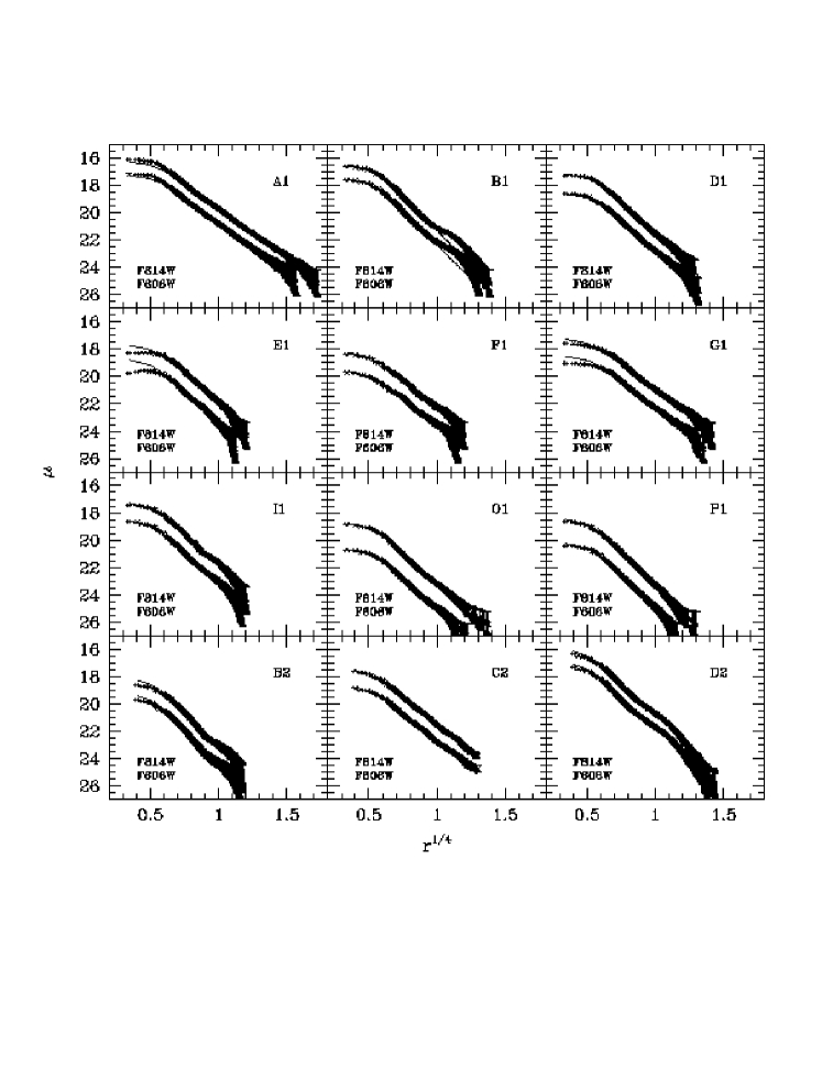
Figure 5: Luminosity profiles, I. The luminosity profiles obtained by isophotal fitting are plotted together with the best-fitting $r^{1/4}\,$model convolved with the PSF. Surface brightness ($\mu$) is plotted in mag arcsec^-2, radius (r) in arcsec. The upper curves represent luminosity profiles through filter F814W, the lower through filter F606W. The profiles of galaxies A1, B1, D1, I1, G1, E1, F1, O1, P1 are taken from T99. Galaxy B1 shows a spiral pattern in the residuals of the two-dimensional fit (see T99). Galaxy D2 is fitted by an $r^{1/4}\,$plus exponential model.

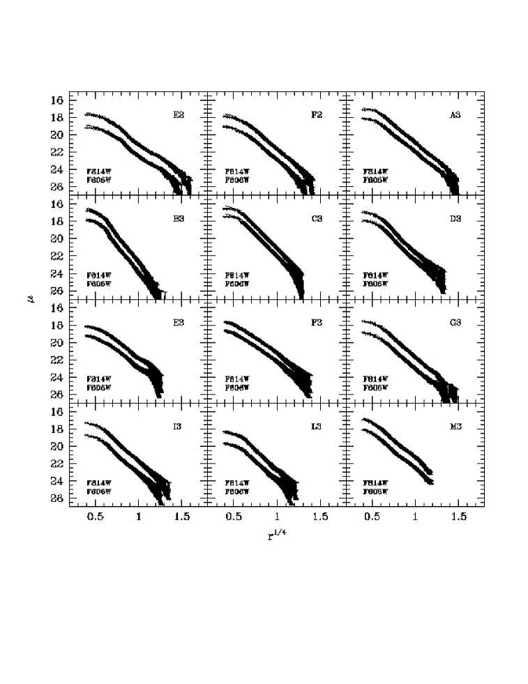
Figure 6: Luminosity profiles, II. As in Figure 5. Galaxy F3 hosts a dust lane in the central region; the profile shown here is corrected for extinction as described in Section 3. Galaxy E3 has a clear spiral pattern, see Figure 15.

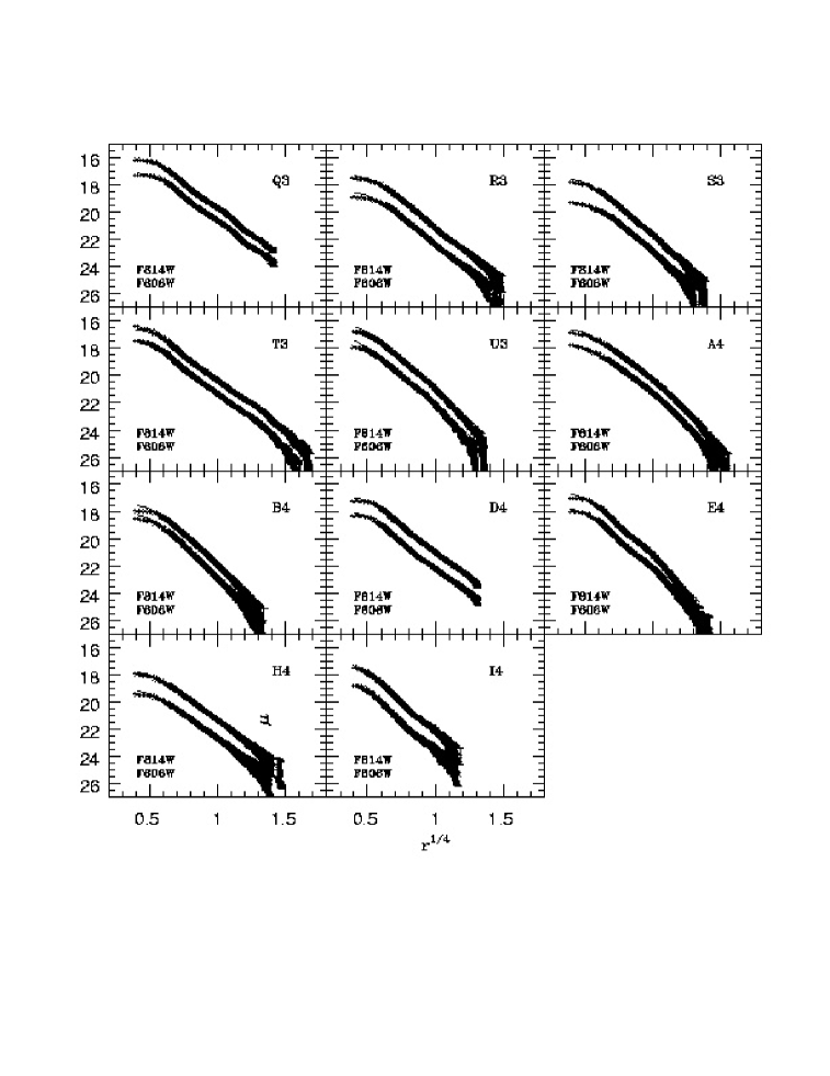
Figure 7: Luminosity profiles, III. As in Figure 5. Galaxies S3 and A4 are fitted by an $r^{1/4}\,$plus exponential model.

3.1 Galactic extinction

We used E(B-V) values given by Schlegel et al. (1998) and the relations $A_{6}=2.889\,\textrm{E(B-V)}$ and $A_{8}=1.948\,\textrm{E(B-V)}$ calculated by Schlegel et al. (1998). The galactic extinction for each field is listed in Table 2. We compared the extinction given by Schlegel et al. (1998) with the values given by Burstein & Heiles (1982). The average difference in E(B-V) is 0.017, consistent with the different zero point used by the authors (see Schlegel et al. 1998), and the scatter is 0.012.

3.2 Rest frame photometric quantities

As in T99, the rest frame photometric quantities are computed from the observed ones using the K-color correction ($\Delta$m_V8, $\Delta$m_B6; listed in Table 4) defined as:

$$\Delta m_{V8}\equiv -2.5\log\Big{[}\int F_{\lambda}(\lambda)S_{V}(\lambda)d\lambda\Big{]}+\textrm{zp}_{V}$$ (5)

$$+2.5\log\Big{[}\int F_{\lambda}(\lambda)S_{\textrm{8}}(\lambda(1+z))d\lambda\Big{]}-\textrm{zp}_{8},$$

$$\Delta m_{B6}\equiv -2.5\log\Big{[}\int F_{\lambda}(\lambda)S_{B}(\lambda)d\lambda\Big{]}+\textrm{zp}_{B}$$ (6)

$$+2.5\log\Big{[}\int F_{\lambda}(\lambda)S_{\textrm{6}}(\lambda(1+z))d\lambda\Big{]}-\textrm{zp}_{6},$$

where zp and $S(\lambda)$ are the zero points and transmissions of the band passes in the Landolt system, while $F_{\lambda}(\lambda)$ is the flux per unit wavelength of the model spectrum. The model spectrum used is the synthetic spectrum (from Bruzual & Charlot 1993; GISSEL96 version) of a single-burst stellar population that best reproduces the observed colour (see T99 and Section 3.3).

Table 4: K-color correction, computed as described in Section 3.2. Errors ($\delta\Delta m_{B6}$ and $\delta\Delta m_{V8}$) are computed as described in Section 3.3.

gal	$\Delta m_{B6}$	$\delta\Delta m_{B6}$	$\Delta m_{V8}$	$\delta\Delta m_{V8}$
A1	1.03	0.05	1.07	0.04
B1	0.97	0.02	1.02	0.02
D1	0.41	0.01	0.85	0.01
E1	0.66	0.02	0.99	0.02
F1	0.62	0.01	0.93	0.01
G1	0.62	0.01	0.93	0.01
I1	0.64	0.02	0.96	0.02
O1	-0.29	0.04	0.65	0.03
P1	-0.06	0.02	0.73	0.01
B2	0.23	0.01	0.80	0.01
C2	0.33	0.01	0.82	0.01
D2	0.85	0.03	0.98	0.02
E2	0.38	0.01	0.85	0.01
F2	0.53	0.01	0.91	0.01
A3	0.75	0.01	0.95	0.01
B3	0.19	0.01	0.80	0.01
C3	1.04	0.01	1.04	0.01
D3	0.89	0.05	0.97	0.04
E3	0.68	0.03	0.94	0.03
F3	0.75	0.02	0.94	0.01
G3	0.36	0.01	0.84	0.01
I3	0.33	0.01	0.85	0.01
L3	0.35	0.01	0.83	0.01
M3	0.52	0.01	0.89	0.01
Q3	0.99	0.02	1.01	0.01
R3	0.50	0.01	0.90	0.01
S3	0.47	0.01	0.87	0.01
T3	1.12	0.02	1.12	0.02
U3	0.78	0.02	0.99	0.02
A4	1.07	0.01	1.08	0.01
B4	0.78	0.01	0.95	0.01
D4	0.66	0.01	0.96	0.01
E4	0.83	0.01	0.96	0.01
H4	0.52	0.01	0.90	0.01
I4	0.54	0.01	0.93	0.01

The radii $r_{\textrm{eB}}$ and $r_{\textrm{eV}}$ are calculated for the central rest wavelength of each filter B and V by linear interpolation/extrapolation in wavelength between the measured radii in the WFPC2 filters F606W and F814W at their observed central wavelengths. We take the central wavelengths of B, V, F606W, and F814W to be 4400, 5500, 5935, and 7921 Å, respectively, resulting in the following formulae for the angular sizes:

$$r_{\textrm{e}{\sc B}}= \big{\{}r_{\textrm{e}{\sc F606W}}[7921-(1+z)4400]$$ (7)

$$+r_{\textrm{e}{\sc F814W}}[(1+z)4400-5935]\big{\}}/1986$$

$$r_{\textrm{e}{\sc V}}= \big{\{}r_{\textrm{e}{\sc F606W}}[7921-(1+z)5500]$$ (8)

$$+r_{\textrm{e}{\sc F814W}}[(1+z)5500-5935]\big{\}}/1986\,.$$

The rest frame surface brightness is computed as:

$$\textrm{SB}_{\textrm{e}{V}}=\textrm{SB}_{\textrm{e}{8}}-10\log(1+z)+\Delta\textrm{m}_{V8}-\textrm{A}_{8}$$ (9)

$$\textrm{SB}_{\textrm{e}{B}}=\textrm{SB}_{\textrm{e}{6}}-10\log(1+z)+\Delta\textrm{m}_{B6}-\textrm{A}_{6}$$ (10)

Table 5 lists for each galaxy the effective radius in kpc, computed for a cosmological model with $\Omega=1$, $\Omega_{\Lambda}=0$, $h_{50}=1$, and the effective surface brightness.

Table 5: Rest frame photometric structural parameters. Effective radii are in $h_{50}^{-1}$kpc (for $\Omega=1$ and $\Omega_{\Lambda}=0$). The error on the rest frame colour B-V is listed as $\delta$BV. The morphological classification (Class; Section 3.4) is also listed. Photometric structural parameters for S0 and S refer to the $r^{1/4}\,$component. Errors are computed as described in Section 3.3.

gal	$SB_{\textrm{eB}}$	$R_{\textrm{eB}}$	$\delta$FPB	$SB_{\textrm{eV}}$	$R_{\textrm{eV}}$	$\delta$FPV	$\delta$BV	Class
A1	$20.54\pm 0.08$	$5.32\pm 0.47$	0.050	$19.67\pm 0.13$	$5.49\pm 0.25$	0.035	0.083	E
B1	$19.81\pm 0.06$	$1.86\pm 0.05$	0.047	$18.90\pm 0.07$	$1.85\pm 0.03$	0.032	0.039	S
D1	$19.80\pm 0.20$	$4.90\pm 0.63$	0.029	$18.76\pm 0.16$	$4.43\pm 0.42$	0.020	0.028	E
E1	$20.79\pm 0.15$	$4.85\pm 0.48$	0.087	$19.92\pm 0.21$	$5.03\pm 0.43$	0.059	0.074	E
F1	$21.54\pm 0.07$	$6.02\pm 0.01$	0.087	$20.56\pm 0.09$	$5.72\pm 0.01$	0.059	0.033	E
G1	$20.78\pm 0.20$	$8.64\pm 1.19$	0.087	$19.80\pm 0.18$	$8.20\pm 0.64$	0.059	0.045	E
I1	$19.97\pm 0.26$	$3.46\pm 0.65$	0.087	$19.07\pm 0.24$	$3.44\pm 0.38$	0.060	0.073	E
O1	$20.38\pm 0.31$	$4.83\pm 0.60$	0.030	$19.24\pm 0.29$	$3.97\pm 1.30$	0.028	0.092	E
P1	$20.11\pm 0.27$	$3.75\pm 0.36$	0.030	$19.22\pm 0.19$	$3.64\pm 0.52$	0.024	0.048	E
B2	$19.62\pm 0.29$	$2.72\pm 0.33$	0.035	$19.26\pm 0.22$	$3.12\pm 0.44$	0.022	0.019	E/S0
C2	$20.21\pm 0.16$	$6.91\pm 0.65$	0.026	$19.42\pm 0.12$	$6.59\pm 0.57$	0.017	0.014	E/S0
D2	$18.68\pm 0.96$	$1.54\pm 1.30$	0.025	$18.08\pm 0.74$	$1.63\pm 0.70$	0.021	0.050	S0
E2	$20.78\pm 0.09$	$10.34\pm 0.51$	0.023	$19.77\pm 0.10$	$9.50\pm 0.51$	0.017	0.017	E/S0
F2	$20.73\pm 0.14$	$5.90\pm 0.55$	0.023	$19.74\pm 0.11$	$5.53\pm 0.31$	0.016	0.016	E/S0
A3	$20.59\pm 0.14$	$5.05\pm 0.61$	0.011	$19.41\pm 0.14$	$4.51\pm 0.33$	0.009	0.010	E/S0
B3	$17.57\pm 0.18$	$1.64\pm 0.06$	0.049	$16.98\pm 0.31$	$1.64\pm 0.19$	0.057	0.050	E
C3	$19.74\pm 0.14$	$1.23\pm 0.22$	0.013	$18.78\pm 0.10$	$1.21\pm 0.13$	0.012	0.021	E
D3	$19.69\pm 0.44$	$1.51\pm 0.53$	0.038	$18.73\pm 0.41$	$1.45\pm 0.29$	0.034	0.078	E
E3	$21.70\pm 0.12$	$6.63\pm 0.80$	0.023	$20.87\pm 0.16$	$6.59\pm 0.51$	0.016	0.074	S
F3	$21.61\pm 0.29$	$7.04\pm 1.66$	0.027	$20.79\pm 0.33$	$6.95\pm 0.92$	0.030	0.033	E/S0
G3	$20.17\pm 0.36$	$5.27\pm 1.06$	0.018	$19.19\pm 0.40$	$5.00\pm 1.10$	0.025	0.012	E
I3	$19.74\pm 0.28$	$4.04\pm 0.70$	0.013	$18.93\pm 0.23$	$4.24\pm 0.64$	0.009	0.058	E/S0
L3	$20.64\pm 0.26$	$4.15\pm 0.63$	0.016	$19.58\pm 0.35$	$3.71\pm 0.72$	0.020	0.094	E/S0
M3	$20.24\pm 0.18$	$5.31\pm 0.79$	0.025	$19.26\pm 0.13$	$4.90\pm 0.47$	0.019	0.015	E
Q3	$20.58\pm 0.10$	$4.19\pm 0.45$	0.025	$19.60\pm 0.07$	$4.03\pm 0.26$	0.017	0.028	E
R3	$20.63\pm 0.12$	$7.18\pm 0.56$	0.009	$19.71\pm 0.21$	$6.94\pm 0.68$	0.012	0.030	E/S0
S3	$21.22\pm 0.29$	$7.03\pm 0.67$	0.052	$19.60\pm 0.07$	$5.21\pm 0.28$	0.009	0.016	S0
T3	$21.05\pm 0.20$	$3.32\pm 0.40$	0.035	$20.30\pm 0.08$	$3.57\pm 0.24$	0.022	0.034	E/S0
U3	$20.38\pm 0.10$	$4.09\pm 0.13$	0.024	$19.46\pm 0.11$	$4.06\pm 0.06$	0.030	0.038	E/S0
A4	$20.85\pm 0.02$	$2.77\pm 0.55$	0.048	$19.75\pm 0.13$	$2.66\pm 0.30$	0.036	0.007	S0
B4	$20.43\pm 0.06$	$2.36\pm 0.15$	0.010	$20.06\pm 0.03$	$2.72\pm 0.08$	0.009	0.011	E/S0
D4	$20.67\pm 0.05$	$6.06\pm 0.32$	0.025	$19.73\pm 0.07$	$5.93\pm 0.20$	0.017	0.011	E/S0
E4	$20.13\pm 0.06$	$2.68\pm 0.23$	0.027	$19.17\pm 0.03$	$2.56\pm 0.12$	0.024	0.024	E/S0
H4	$21.17\pm 0.10$	$9.73\pm 0.71$	0.080	$20.25\pm 0.10$	$9.33\pm 0.38$	0.054	0.043	E
I4	$20.26\pm 0.38$	$3.80\pm 0.98$	0.081	$19.43\pm 0.24$	$3.82\pm 0.53$	0.054	0.051	E/S0

3.3 Error analysis

The main sources of error are given by:

1. Fitting technique. We estimate the error in terms of the half-difference of the values found with the two independent fitting techniques used (luminosity profiles and 2Dl$\chi^{2}$ fitting).

2. PSF modelling. We estimate this effect by fitting a small galaxy in the corner of the chip (D3) and a large one in the centre of the chip (H4) with a set of different PSFs. We use a Tiny Tim PSF generated on the galaxy position, a star present on the chip, and a Tiny Tim PSF generated on the position of the star. For D3, which is observed on three frames with different subpixel pointings, we produce a PSF by summing three subsampled PSFs centred on the corresponding position within the pixel. The r.m.s. scatter of the effective radius derived with the various PSFs is 3 per cent for D3 and 2 per cent for H4 and the scatter of $FP_{ph}$ is respectively 0.007 and 0.004. Therefore, this is a negligible source of error for our purposes.

3. Sky subtraction and flat fielding. We measured the contribution to the error given by these uncertainties by varying the background by 1 per cent (which we take as upper limit to the errors in sky subtraction and flat fielding) and by running the 2D fits. These errors are smaller than the ones due to the fitting technique, but in some cases they are not negligible.

4. Galactic extinction. We adopt the error estimate by Schlegel et al. (1998) for the reddening correction $\delta$E(B-V)=0.16E(B-V).

5. K-color correction. For each galaxy, we computed the colours of single-burst stellar population spectra (Bruzual & Charlot 1993; GISSEL96 version) with ages between 0.5 and 20 Gyr, redshifted to the galaxy redshift. We also computed K-color corrections for each synthetic spectrum. By interpolation we found the K-color correction corresponding to the colour of each galaxy. This procedure applied to the colours shifted by a standard deviation provided upper and lower limits to the K-color correction. The error on the K-color correction is the half-difference of the upper and lower limits. Table 4 lists the K-color corrections ($\Delta$m_B6 and $\Delta$m_V8) together with their errors ($\delta\Delta$m_B6 and $\delta\Delta$m_V8).

The total error on the measured parameters listed in Table 3 is the quadratic sum of terms i and iii. The uncertainties on the extinction correction and on the K-color correction are added in quadrature to produce the total errors listed in Table 5. The systematic uncertainty in the zero point is not considered here and will be taken into account when comparing the intermediate redshift results to the local ones in PIII.

3.4 Classification

The objects are classified in a simplified scheme (E, E/S0, S0, S) based on their morphology and luminosity profile. Among the early-type systems, objects that are best-fitted by a pure $r^{1/4}\,$  profile are classified as E; objects for which the addition of an exponential component gives a slightly better fit with no significant change in the structural parameters are classified as E/S0; objects that are significantly better described by an $r^{1/4}\,$plus exponential profile are classified as S0. Objects that show a spiral pattern (B1, E3) are classified as S. The classification is listed in Table 5. Note that in this classification the usage of the symbol E/S0 is different with the respect to the rest of the paper, where it indicates the entire class of early-type galaxies.

4 Spectroscopy

A total of 13 dark nights at the ESO 3.6m telescope were awarded for this spectroscopic project.

The first pilot observing run (run 1, described in T99) took place in 1996, April 18-22. Long slit ($1\aas@@fstack{\prime\prime}5$ slit width) spectroscopy was obtained with the EFOSC spectrograph, with the Orange 150 grism in the spectral range between approximately 5200 and 7000 Å  ($512\times 512$ CCD, with pixel size $30\mu m$ equivalent to about $3.5\textrm{\AA}\times 0\aas@@fstack{\prime\prime}57$). The estimated seeing, measured with R-band acquisition images, was $0\aas@@fstack{\prime\prime}8$ FWHM.

The following runs (run 2, 3, 4) took place in 1999, March 19-21, August 11-14, and November 2-6. The imager-spectrograph EFOSC2 was used with grism # 9, which covers the range 4700-6700 Å, with pixel size of approximately 2Å$\times 0\aas@@fstack{\prime\prime}32$ in $2\times 2$ binning mode. A narrower slit ($1^{\prime\prime}$) was used in order to achieve a better resolution. The seeing ranged from $0\aas@@fstack{\prime\prime}8-\aas@@fstack{\prime\prime}2$ during run 2 and 3. Run 4 was subject to highly variable weather conditions: two nights were lost for clouds and bad seeing ($2-3^{\prime\prime}$), one night had average seeing conditions (0$\aas@@fstack{\prime\prime}8-1^{\prime\prime}$), and during the last night we had some episodes of excellent seeing (image quality 0$\aas@@fstack{\prime\prime}$6).

He-Ar lamps in the pointing position were taken before and after every set of 2 exposures to provide accurate wavelength calibration. Standard stars were observed at the beginning and at the end of every night to provide relative flux calibration.

The spectra were reduced as described in T99 (see also Treu 2001). For every galaxy, Table 1 gives total integration time, number of exposures, S/N achieved. In Figures 8 to 9 the spectra with highest signal-to-noise collected are shown. The run is identified by the digit in the name. The spectra taken during run 1, shown in T99, are not repeated here.

Figure 8: Wavelength calibrated spectra of the galaxies with average S/N per pixel greater than 10 taken with EFOSC2, I. The shaded spectral regions were affected by strong sky-emission lines. These regions have not been used in the kinematic fit. The standard deviation per pixel is also shown (lower curves). The Calcium doublet (Ca H 3968.5 Å  and K 3933.7 Å), the G band (4304.4 Å), H$\beta$, and Mg_b (5175.4 Å) are the most prominent absorption features in this spectral region. Note the extremely strong Balmer absorption features in the spectrum of B3 and the NaD (5892.5 Å) line in the spectrum of the lowest redshift objects such as C3. Note [OII]3727 (Å)in emission in the spectrum of E2. The central velocity dispersion in kms^-1 is shown in the upper left corner when measured (see Section 4).

Figure 9: Wavelength calibrated spectra of the galaxies with average S/N per pixel greater than 10 taken with EFOSC2, II. See caption to Figure 8.

For runs 2, 3, and 4, by taking advantage of the higher number of spectra available with the same instrumental setup, we were able to determine the resolution of our final combined spectra more accurately than in run 1 (see T99). We selected a set of 3 sky lines and 12 He-Ar lines that are unblended at our resolution and sufficiently strong and isolated and we measured their FWHM on each combined sky and He-Ar calibration spectrum. The results were very stable from frame to frame and from sky to He-Ar lines, so we fitted the entire set of measurements as a function of wavelength. The measurements of the resolution ($\sigma_{s}$ in km $\textrm{s}^{-1}$) are well fitted by a parabola, as shown in Figure 10, left panel.

Figure 10: Left: resolution ($\sigma_{s}$) as a function of wavelength as determined from the width of sky and He-Ar lines for the EFOSC2 setup. Right: resolution ($\sigma_{t}$) as a function of wavelength for the SK stellar template library (the points represent the measured resolution, the solid line is the best fitting parabola; see Table 6 and Section 4.2); the resolution of the JHC library (4.76Å  see Section 4.2) is shown for comparison as a dashed line.

4.1 Fitting kinematic parameters

The internal velocity dispersion is derived by comparison of the observed galaxy spectrum to a stellar spectrum taken with the same resolution under the assumption that the galaxy spectrum can be well described by the sum of the spectra emitted by stars with a Gaussian velocity distribution.

In the first exploratory study (T99) we derived kinematic information for our sample of galaxies with two different and independent methods: i) the Gauss-Hermite Fourier Fitting Software (Franx, Illingworth & Heckman 1989; van der Marel & Franx 1993), hereafter GHFF, and ii) the Fourier Quotient (Sargent et al. 1977) in the version modified by Rose (see Dressler 1979) and by Stiavelli, Møller & Zeilinger (1993). The results of the two methods were mutually consistent, within the estimated errors. However, the GHFF allows for a reliable estimate of the errors, is less sensitive to template mismatches (van der Marel & Franx 1993), and provides insight in the fitting procedure. Finally, it provides a quality parameter (the $\chi^{2}$) and the residual spectrum. Therefore, here we will use only the GHFF software.

4.2 Stellar templates

A good library of stellar spectra is a key ingredient to measure the internal kinematics of a galaxy. It has to cover the largest possible range of spectral types so that stellar population effects can be studied. In addition, the spectral resolution of the stellar template ($\sigma_{t}$) must be better than the instrumental resolution of the setup used for galactic spectroscopy. The stellar library used in T99 (Jacoby, Hunter & Christian 1984; hereafter the JHC library), given its resolution ($\sim$ 4.5 Å  FWHM, i.e. $\sigma_{t}=133$ km $\textrm{s}^{-1}$at 4300 Å), can only be used out to $z\sim 0.2$ with our spectroscopic setup.

David Soderblom and Jeremy King kindly provided us with a library of stellar spectra at higher resolution for the highest redshift part of the sample (hereafter the SK library). The stars, listed in Table 6, were observed at the Kitt Peak National Observatory Coudé Feed Telescope, with the Coudé CCD Spectrograph, on May 22 1999. The stars were chosen according to observability from a list of giant stars covering all spectral types from A0 to K7. In addition, a few dwarf star spectra were also taken. The spectral range covered is 3120–5510 Å. The resolution of the SK library, as measured from calibration lamps, is shown in Figure 10, right panel.

Table 6: Stars observed as stellar templates (SK library; see Section 4.2 for details). For each star we list the spectral type, name of the star, magnitude and colour, taken.

type	star	V	B-V
A2III	HR4343	4.48	0.03
A9III	HR4584	6.50	0.22
F3III	HR5783	6.45	-
F5III	HR4191	5.18	0.33
F9III	HR4451	6.05	0.60
G4III	HR4255	5.66	0.83
G4III	HR4558	5.30	0.88
G5III	HR3922	5.93	0.89
G8III	HR5888	5.23	1.02
G8III	HR6770	4.64	0.96
G9III	HR4609	5.80	1.01
K0III	HR4287	4.08	1.09
K2III	HR6299	3.20	1.15
K3III	HR4365	5.32	1.20
K3III	HR4521	5.27	1.27
K6III	HR4672	5.81	1.30
K7III	HR6159	4.84	1.49
F5V	HR4657	6.11	0.46
F9V	HR4540	3.61	0.55
G0V	HR4845	5.95	0.55

Unfortunately, the limited red coverage of the spectra in the SK library did not allow us to use them for the low redshift objects of the sample ($z<0.21$). Therefore, we used the JHC library for the low redshift part of the sample ($z<0.21$) and the SK library for the high redshift part of the sample ($z>0.21$).

In order to derive an accurate and consistent value for the resolution of the JHC library, we measured it using the SK library. We divided the overlapping region (3510-5510 Å) into four intervals of 500 Å  each and we fitted the “velocity dispersion” of each interval of the JHC spectra using the SK template that more closely matches the spectral type. By adding in quadrature the resolution of the SK library, we found the intrinsic resolution of the JHC library ($4.76\pm 0.30$ Å  FWHM), in agreement with the value given by Jacoby et al. (1984). We used this value as intrinsic resolution of the JHC library.

The stellar templates were redshifted to the redshift of each object and then broadened with a Gaussian characterized by a width equal to the quadratic difference between the instrumental resolution ($\sigma_{s}$) and the resolution of the template library ($\sigma_{t}$).

4.3 Results and error discussion

As in T99, we fitted each galaxy with each of the stellar templates available. This procedure allows us to estimate the uncertainty given by template mismatches. As noted in T99, the late G to early K giant stars provided the best $\chi^{2}$, the smallest residual, and the most stable results. Cooler stars produced systematically higher velocity dispersions and hotter stars systematically lower ones.

As best estimate of the velocity dispersion and redshift ($\sigma_{\textrm{ghff}}$ , $z_{\textrm{ghff}}$   in Table 7), we adopted the average of the values obtained with templates in the spectral range G4-K0III. In order to achieve homogeneous results with the two libraries, we used the same number of templates and closely matching spectral type distributions: 2xG4, 1xG5, 2xG8, 1xG9, 1xK0 for SK and 1xG5, 2xG6, 1xG7, 1xG8, 1xG9, 1xK0 for JHC. In Table 7 we also list the best-fitting template for each galaxy. Note that the best-fitting template spans the entire range of spectral types. Two estimates of the errors are also given, as in T99: the random component, which is the fit formal uncertainty obtained for the best-fitting template ($\delta$); the systematic component ($\Delta$), resulting from template mismatches, computed as the r.m.s. scatter of the values obtained with different templates.

Table 7: Kinematic results from the GHFF fit. For each galaxy we list the average velocity dispersion ($\sigma_{\textrm{ghff}}$ ) together with the random error ($\delta$$\sigma_{\textrm{ghff}}$ ) and the systematic error ($\Delta$$\sigma_{\textrm{ghff}}$ ). The random error is the fit formal uncertainty for the best-fitting template, while $\Delta$$\sigma_{\textrm{ghff}}$   is the scatter of the values obtained with the templates in the range G4-K0 III (see Section 4.3). We also list the redshift ($z_{\textrm{ghff}}$ ) with its errors, the spectral type of the best-fitting template (Type), the signal-to-noise ratio (S/N), and the matching to the relevant selection criteria (sel; see Section 2.3). Only galaxies with $\textrm{S/N}>12$ are listed (see Section 4.3). The values of velocity dispersion found for B1, D2, E3, Q3, B4, E4 are too small to be acceptable (see discussion in Section 4.3): these objects have been excluded from the table.

gal	$\sigma_{\textrm{ghff}}$	$\delta\sigma_{\textrm{ghff}}$	$\Delta$$\sigma_{\textrm{ghff}}$	$z_{\textrm{ghff}}$	$\delta$ $z_{\textrm{ghff}}$	$\Delta$ $z_{\textrm{ghff}}$	Type	S/N	sel
A1	227	16	14	0.1466	4.3$\cdot 10^{-5}$	1.2$\cdot 10^{-4}$	G8	65	2
D1	290	21	12	0.3848	6.8$\cdot 10^{-5}$	1.4$\cdot 10^{-4}$	G4	22	2
E1	198	25	7	0.2940	8.4$\cdot 10^{-5}$	1.3$\cdot 10^{-4}$	K0	17	2
G1	220	17	10	0.2946	5.9$\cdot 10^{-5}$	1.3$\cdot 10^{-4}$	G8	35	2
I1	190	20	4	0.2929	6.5$\cdot 10^{-5}$	1.3$\cdot 10^{-4}$	G5	22	2
E2	219	12	3	0.3977	4.4$\cdot 10^{-5}$	1.4$\cdot 10^{-4}$	G4	24	2
F2	237	14	14	0.3364	5.3$\cdot 10^{-5}$	1.3$\cdot 10^{-4}$	G9	18	2
A3	189	15	4	0.2311	4.9$\cdot 10^{-5}$	1.2$\cdot 10^{-4}$	G5	19	2
C3	146	15	9	0.1057	3.8$\cdot 10^{-5}$	1.4$\cdot 10^{-4}$	G8	27	2
D3	136	18	8	0.1511	4.8$\cdot 10^{-5}$	1.0$\cdot 10^{-4}$	G9	17	0
G3	244	11	7	0.4081	4.5$\cdot 10^{-5}$	1.4$\cdot 10^{-4}$	G5	21	2
I3	194	11	8	0.4103	4.1$\cdot 10^{-5}$	1.4$\cdot 10^{-4}$	G5	22	2
L3	193	18	15	0.4141	6.8$\cdot 10^{-5}$	1.4$\cdot 10^{-4}$	G5	13	1
M3	228	15	5	0.3374	5.4$\cdot 10^{-5}$	1.4$\cdot 10^{-4}$	G4	16	2
R3	228	11	5	0.3482	4.0$\cdot 10^{-5}$	1.3$\cdot 10^{-4}$	G5	24	2
S3	216	19	5	0.3559	7.2$\cdot 10^{-5}$	1.1$\cdot 10^{-4}$	G4	18	2
T3	133	23	16	0.1174	5.2$\cdot 10^{-5}$	1.0$\cdot 10^{-4}$	G6	14	2
U3	238	14	21	0.2401	5.2$\cdot 10^{-5}$	1.2$\cdot 10^{-4}$	G9	18	0
A4	167	15	8	0.1171	4.1$\cdot 10^{-5}$	1.2$\cdot 10^{-4}$	G7	25	2
D4	224	15	11	0.2848	5.1$\cdot 10^{-5}$	1.2$\cdot 10^{-4}$	G4	32	2
H4	217	12	5	0.3399	4.4$\cdot 10^{-5}$	1.4$\cdot 10^{-4}$	G9	25	2
I4	243	20	13	0.3369	7.2$\cdot 10^{-5}$	1.3$\cdot 10^{-4}$	G4	19	2

It is intuitive and well known (e.g. Bender 1990; Jørgensen, Franx & Kjærgaard 1995; T99) that the S/N needed to measure velocity dispersions properly scales with the ratio between the instrumental resolution and the velocity dispersion itself. In other words, when the velocity dispersion is smaller than the instrumental resolution a higher minimum signal-to-noise is needed with respect to the case when the velocity dispersion is larger than the instrumental resolution.

In practice, for any given S/N and resolution, there is a lower limit on the velocity dispersion measurable without introducing significant bias (for example, Bender 1990 considers half of the instrumental resolution to be the minimum measurable value). Quantitatively, these numbers depend on the instrumental setup (resolution, sampling). Therefore, we addressed the problem by numerical simulation of our measurement procedure. For a range of values of velocity dispersions ($\sigma_{\textrm{in}}=65$, 75, 100, 125, 150, 175, 200 km $\textrm{s}^{-1}$) and of S/N (10, 12, 15, 18, 25), we created 1000 toy galaxy spectra with artificial noise and our instrumental sampling and resolution. We then recovered the velocity dispersion with the GHFF software. The results are plotted in Figure 11.

Figure 11: Results of Montecarlo simulations for the EFOSC2 setup. For a range of values of velocity dispersion ($\sigma_{\textrm{in}}$) the velocity dispersion recovered is plotted as a function of S/N (using the same star as “galaxy” and template in panel a, and using a different star as template in panel c). The scatter of the distribution is plotted in panels b (same star as template and galaxy) and d (different star as template and galaxy). At $\textrm{S/N}<15$ velocity dispersions below 100 km $\textrm{s}^{-1}$  are systematically underestimated. Moreover, for small velocity dispersions, the uncertainty is large even for higher values of S/N.

For each input value of $\sigma_{\textrm{in}}$ we plot the average recovered $\sigma$ as a function of S/N, using the same stellar spectrum as “galaxy” and template (G8 III; panel a) or using a different star as template (G9 III; panel c). It is noticed that the smallest values of $\sigma_{\textrm{in}}$ are systematically underestimated by the fit for low values of S/N (by as much as 13 per cent for $\sigma_{\textrm{in}}=65$ km $\textrm{s}^{-1}$  and $\textrm{S/N}=10$) but for $\sigma_{\textrm{in}}>100$ km $\textrm{s}^{-1}$  the effect becomes negligible ($<2$ per cent at $\textrm{S/N}=10$, $<1$ per cent at $\textrm{S/N}=12$ for $\sigma_{\textrm{in}}=100$ km $\textrm{s}^{-1}$  and using a different template). If – instead of the average of $\sigma$ – the average of the logarithm of $\sigma$ weighted on the formal variance is used as estimator (Jørgensen et al. 1995), the effect is reversed: the velocity dispersion is now overestimated for small values of $\sigma_{\textrm{in}}$ (by up to 15 per cent at $\sigma_{\textrm{in}}=65$ km $\textrm{s}^{-1}$and $\textrm{S/N}=10$). In addition, high values of $\sigma_{\textrm{in}}$ (from 200 km $\textrm{s}^{-1}$  in our simulation) become underestimated by 2 per cent at $\textrm{S/N}=10$. The conclusion is that the systematic uncertainty on small values of S/N is hard to correct, so that it is suggested that these data should be rejected. In our particular case we will only accept for measurement spectra with $\textrm{S/N}>12$ (thus rejecting F1, B3, F3). In Figure 11 we also plot the relative scatter around the mean for the same configurations (template G8 III, panel b; template G9 III, panel d). For a given S/N the uncertainty on the velocity dispersion increases dramatically for the smallest values of $\sigma_{\textrm{in}}$, while it tends to become constant for velocity dispersions much larger than the resolution. This is consistent with what we find for galaxies B4 and E3 ($\sigma_{\textrm{ghff}}$  $=64$ and 98 km $\textrm{s}^{-1}$): despite the good S/N of the spectrum the formal uncertainty on $\sigma_{\textrm{in}}$ is $\sim 35$ and $\sim 18$ per cent. We do not consider these values to be successfully measured. Similarly, the small value of velocity dispersion of galaxy B1 was rejected in T99.

Since most of the objects at $z<0.21$ have high S/N spectra, the problems discussed above are negligible. Nevertheless, the uncertainty in the JHC spectral library resolution ($\sim 120\pm 8$ km $\textrm{s}^{-1}$  at 5000 Å) can cause systematic effects on the low velocity dispersion objects. We ran extensive simulations (as above) to measure this effect. For velocity dispersions smaller than the resolution of the library, the uncertainty is important (for example $\sim 10$ per cent at 100 km $\textrm{s}^{-1}$  with $\textrm{S/N}=25$), but it drops quickly with increasing velocity dispersion (6 per cent at 125 km $\textrm{s}^{-1}$  with $\textrm{S/N}=25$; 4 per cent at 150 km $\textrm{s}^{-1}$). In practice, at $\sigma_{\textrm{in}}=125$ km $\textrm{s}^{-1}$  this effect is already smaller than the typical uncertainty. We will not consider galaxies D2, Q3, E4 as successfully measured because their velocity dispersion is smaller than this limit.

The uncertainty in the measurement of the instrumental resolution of EFOSC ($\Delta\lambda=8.39\pm 0.26$Å) introduces a systematic error in the measurement of the velocity dispersion that is negligible in our case. For example, let us consider A1, the galaxy with the highest signal-to-noise spectrum. The random error is estimated to be 6 per cent, the systematic error due to template mismatches is 7 per cent; therefore, the additional 3 per cent associated with the uncertainty in the measurement of instrumental resolution, to be added in quadrature, does not change the total error significantly. As a check, we repeated the fits with templates broadened to the resolution changed by a standard deviation. For galaxy I1 we obtained the largest difference (7 km $\textrm{s}^{-1}$), still negligible with respect to the other sources of error. The effect on the uncertainty on the resolution of EFOSC2 is smaller and totally negligible.

The spectra of galaxies D1, E2, F2, G3, I3, L3, M3, R3, S3, U3, D4, H4, and I4 include the lines Ca H and K. As noted in T99, even though widely used to perform such measurements (Dressler 1979), these lines have been reported to induce a slight overestimate of the velocity dispersion (Kormendy 1982; see also Kormendy & Illingworth 1982). Kormendy & Illingworth (1982) suggest that the problem may be caused by the intrinsic width of the lines or by the steepness of the continuum in that spectral region. However, Dressler (1984) suggests that they may be best suited for the measurement of large velocity dispersions for faint objects, such as D1. For these reasons, we performed the kinematic fit also by masking the region of Ca H and K. In Figure 12 the variation of $\sigma$ as a function of velocity dispersion and S/N is plotted. The velocity dispersion obtained with Ca H and K, as listed in Table 7, is on average 1.4 per cent higher than the one obtained by masking this region, with a 6.6 per cent scatter. The effect is within the estimated error and the scatter is likely to be induced by the loss of information caused by masking a significant part of the spectrum. We conclude that with this kind of resolution, sampling, signal-to-noise ratio, and treatment of the continuum, the presence of Ca H and K does not alter significantly the measurement of velocity dispersion.

Figure 12: Relative difference in velocity dispersion as measured with and without Ca H and K as a function of velocity dispersion (upper panel) and average S/N per pixel (lower panel). The error bars are the quadratic sum of the systematic and random errors, as defined in the Section 4.3. The average difference is 1.4 per cent with a scatter of 6.6 per cent. The average difference is negligible with respect to the errors (see Table 7) and consistent with the scatter found.

Figure 13: Relative difference in velocity dispersion as measured with and without NaD as a function of velocity dispersion (upper panel) and average S/N per pixel (lower panel). The error bars are the quadratic sum of the systematic and random errors, as defined in the Section 4.3. The average difference is 2.3 per cent, negligible with respect to the errors (see Table 7).

Similarly, the spectra of A1, C3, T3, and A4 include the region of NaD, which may be affected by interstellar absorption even in elliptical galaxies (e.g. Dressler 1984). We repeated the analysis by excluding the NaD region (see Figure 13) and found an average velocity dispersion higher by 2.3 per cent. As above, we conclude that the presence of NaD in the spectrum does not alter significantly the result, and used in Table 7 the values found by using the entire spectral range.

The total error on the redshift, taking into account the error on wavelength calibration, is less than 0.0005, when the GHFF fit was performed and less than 0.002 in the cases where the redshift has been measured by identifying the main spectral features.

4.4 Aperture correction

Spatially resolved kinematics measurements in nearby galaxies (e.g., Capaccioli et al. 1993; Carollo & Danziger 1994a,b; Bertin et al. 1994) have shown that the velocity dispersion varies (generally it declines) with radius. For this reason, central velocity dispersion is generally different from the velocity dispersion measured from the spectrum integrated over the entire galaxy, as is generally available at intermediate redshift. A correction is thus required. As in T99, we model the velocity dispersion profile with a power law,

$$\sigma(r)\propto\left(\frac{r}{r_{e}}\right)^{d},$$ (11)

with $-0.1<d<0$. The desired correction can be computed numerically from

$$\sigma^{2}({\mathcal{A}})\simeq\int_{\mathcal{A}}2\pi rdr\sigma^{2}(r)DV(r).$$ (12)

Here we have assumed that the value obtained by measuring $\sigma^{2}$ within an aperture ${\mathcal{A}}$ is the average of $\sigma^{2}(r)$ weighted by the luminosity density, modelled as an $r^{1/4}\,$law appropriately normalized and indicated by $DV(r)$. With respect to T99, the way we compute the correction has been improved by taking into account the effect of seeing. The effect of seeing is to smear the dependence of the correction on $r_{\textrm{e}}$, whenever the two quantities are comparable. We computed the correcting factor ${\mathcal{B}}(d)=\sigma/$$\sigma_{\textrm{ghff}}$   to an equivalent aperture of radius $r_{\textrm{e}}/8$ (see Jørgensen et al. 1995; T99) for a range of values of seeing ($0\aas@@fstack{\prime\prime}8-1\aas@@fstack{\prime\prime}2$), effective radius (0$\aas@@fstack{\prime\prime}5-2^{\prime\prime}$), and number of lines used. The average correcting factor, computed as ${\mathcal{B}}\equiv[{\mathcal{B}}(-0.1)+{\mathcal{B}}(0)]/2$, ranges from 1.055 to 1.075. The uncertainty related to the intrinsic variety of velocity dispersion profiles (modelled by $d$) is larger than this interval. Therefore, we adopt the mean correcting factor ${\mathcal{B}}=1.065\pm 0.037$, where the error is estimated as ${\mathcal{B}}\equiv[{\mathcal{B}}(-0.1)-{\mathcal{B}}(0)]/2\sqrt{3}$ as in T99. The values obtained for the central velocity dispersion are shown in Figures 8 and 9 together with the spectrum of each galaxy.

4.5 Relative flux calibration

The instrumental response was measured at the beginning and at the end of every night, by observing spectrophotometric standard stars at parallactic angle through a $5^{\prime\prime}$ slit. The response was stable from night to night within 2-3 per cent over the entire spectral range when the same star was used for calibration. Different stars provided similar responses within 5  per cent. We used the average response function to correct the spectra. We estimate the relative flux calibration uncertainty to be $\sim 5$ per cent, dominated by the systematic differences found when different stars are used.

5 Summary

In this paper we have presented the surface photometry and spectroscopy of a sample of HST selected early-type galaxies. The sample is chosen mainly based on morphology and colour. As described in Section 2, our sample is a fair sample of the early-type galaxies found in the Medium Deep Survey, with respect to morphological selection, colour distribution, bulge-to-total luminosity distribution, and luminosity distribution. As already noticed by other authors (see, e.g., Totani & Yoshii 1998), at any given redshift early-type galaxies span a significant range of colours, from the red envelope of old cluster ellipticals bluewards (Figure 2).

In Section 3 we have presented the surface photometry of 35 objects in the redshift range $z=0.11-0.65$ (see Figure 14). The photometric structural parameters (effective radius and effective surface brightness) have been derived with two different techniques: isophote profile fitting ($r^{1/4}\,$and $r^{1/4}\,$+ exponential disc) and 2 dimensional fitting ($r^{1/4}\,$only). The value of the structural parameters changes significantly (r.m.s scatter of 15 per cent in $r_{\textrm{e}}$) with the different modelling, but the combination of effective radius and surface brightness that enters the FP is remarkably stable (r.m.s. scatter 0.03).

In Section 4 we have described spectroscopic measurements obtained at the ESO-3.6m telescope. Redshifts are obtained for all the 35 objects with measured surface photometry. Using Montecarlo simulations, we have studied extensively the systematic errors in the measurement of $\sigma$, due to instrumental resolution and finite S/N. The systematic errors are found to be significant for values of $\sigma$ comparable to the instrumental resolution and for small S/N. Based on these simulations, we measure velocity dispersion only on the 28 spectra with average S/N per pixel larger than 12, and we reject all values of $\sigma<125$ km $\textrm{s}^{-1}$. In the end, we have obtained robust determination of velocity dispersion for 22 galaxies.

A range of stellar templates is used to recover the internal velocity dispersion; the best-fitting template is found to span the entire range G4-K0 III. In this way, we are able to investigate the systematic errors induced by the mismatch between the galactic stellar population and the stellar template used. The average error on internal velocity dispersion is found to be 8 per cent (plus 5 per cent systematic). No significant offset in the average velocity dispersion is found when Ca H and K and NaD lines are masked in the kinematic fit.

Figure 14: Distribution of redshift for the sample galaxies (empty histogram). The galaxies with measurable velocity dispersion ($\textrm{S/N}>12$) are plotted as hatched histogram. The velocity dispersions smaller than our resolution limit were rejected based on Montecarlo simulations (see Section 4.3). The galaxies with measured velocity dispersion are plotted as filled histogram.

6 Acknowledgments

This work is based on observations collected at the European Southern Observatory (La Silla) under programmes 62.O-0592, 63.O-0468, and 64.O-0281 and with the NASA/ESA Hubble Space Telescope, obtained at the Space Telescope Science Institute, which is operated by Association of Universities for Research in Astronomy, Inc. (AURA), under NASA contract NAS5-26555. Tommaso Treu was financially supported by the Space Telescope Science Institute Director Discretionary Research Fund grant 82228 and by the Italian Ministero dell’Università e della Ricerca Scientifica e Tecnologica. The use of the Gauss-Hermite Fourier Fitting Software developed by R. P. van der Marel and M. Franx is gratefully acknowledged. We are grateful to David Soderblom and Jeremy King for providing us with the library of stellar templates used in the kinematic measurement. We thank R. J. Smith for his comments that improved the presentation of the results.

Appendix A Images of noteworthy galaxies

In this appendix we show the images of the two noteworthy galaxies E3 and F3. Galaxy E3 shows a clear spiral pattern in the residuals. The center of galaxy F3 is obscured by a dust lane; the luminosity profile has been measure by correcting the dust extinction as described in Section 3. The images of all the galaxies are available at the MDS world wide web site at URL http://archive.stsci.edu/mds/.

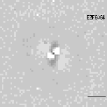
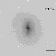
Figure 15: WFPC2 images and 2D fit residuals of secondary target F3. The horizontal bar is 1 arcsec long.

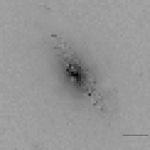
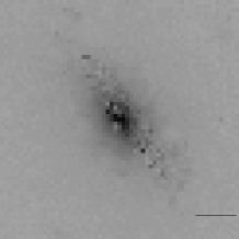
Figure 16: WFPC2 images and 2D fit residuals of galaxy F3. The first line shows the F606W images, the image corrected for dust extinction (see Section 3), and the residuals from the 2D fit. The same images are shown for filter F814W on the second line. The horizontal bar is 1 arcsec long. The noise in the central part of the images on the second and third column is higher than the rest, because of the additional noise due to the internal extinction correction.

References

- [Abrahm et al. 1996] Abraham R. G., van den Bergh S., Glazebrook K., Ellis R. S., Santiago B. X., Surma P., Griffiths R. E., 1996, ApJS, 107, 1
- [Bender 1990] Bender R., 1990, A&A, 229, 441
- [Bertin et al. 1994] Bertin G., Bertola F., Danziger J., Dejonghe H., Sadler E., Saglia R. P., 1994, A&A, 292, 381
- [Bruzual & Charlot 1993] Bruzual A. G., Charlot S., 1993, ApJ, 405, 538
- [Burstein & Heiles 1982] Burstein D., Heiles C., 1982, AJ, 87, 1165
- [Capaccioli et al. 1993] Capaccioli M., Cappellaro E., Held E. V., Vietri M., 1993, A&A, 274, 69
- [Cardelli et al. 1999] Cardelli J., Clayton G., Mathis J., 1989, ApJ, 345, 245
- [Carollo & Danziger 1994a] Carollo C. M., Danziger I. J., 1994a, MNRAS, 270, 523
- [Carollo & Danziger 1994b] Carollo C. M., Danziger I. J., 1994b, MNRAS, 270, 743
- [Djorgovski & Davis 1987] Djorgovski S., Davis M., 1987, ApJ, 313, 59
- [Dressler 1979] Dressler A., 1979, ApJ, 231, 659
- [Dressler 1984] Dressler A., 1984, ApJ, 286, 97
- [Dressler et al. 1987] Dressler A., Lynden-Bell D., Burstein D., Davies R. L., Faber S. M., Terlevich R. J., Wegner G., 1987, ApJ, 313, 42
- [Franx, Illingworth & Heckman 1989] Franx M., Illingworth G. D., Heckman T., 1989, ApJ, 344, 613
- [Griffiths et al. 1994] Griffiths E. et al. 1994, ApJ, 435, L19
- [Jacoby et al. 1984] Jacoby G. H., Hunter D. A., Christian C. A., 1984, ApJS, 56, 257
- [Jørgensen et al. 1995] Jørgensen I., Franx M., Kjærgaard P., 1995, MNRAS, 276, 1341
- [Kelson et al. 2000] Kelson D. D., Illingworth G. D., van Dokkum P. G., Franx M., 2000, ApJ, 531, 137
- [Kormendy 1977] Kormendy J., 1977, ApJ, 218, 333
- [Kormendy 1982] Kormendy J., 1982, Saas-Fee Lectures 12, p. 115
- [Kormendy & Illingworth 1982] Kormendy J., Illingworth G. D., ApJ, 1982, 256, 460
- [Krist 1994] Krist J., 1994, The Tiny Tim User’s Manual, version 4.0. STScI, Baltimore
- [Marzke et al. 1998] Marzke R. O., da Costa L. N., Pellegrini P. S., Wilmer C. N. A., Geller M. J., 1998, ApJ, 503, 617
- [Pahre et al. 1998] Pahre M. A., Djorgovski S. G., De Carvalho R. R., 1998, AJ, 116, 1591
- [Ratnatunga et al. 1999] Ratnatunga K. U., Griffiths R. E., Ostrander E. J., 1999, AJ, 118, 86
- [Salpeter 1955] Salpeter E., 1955, ApJ, 121, 161
- [Sargent et al. 1977] Sargent W. L. W., Schechter P. L., Boksenberg A., Shortridge K., 1977, ApJ, 212, 326
- [Schade et al. 1999] Schade D. et al., 1999, ApJ, 525, 31
- [Schechter 1976] Schechter P., 1976, 203, 297
- [Schlegel et al. 1998] Schlegel, D. J., Finkbeiner D. P., Davis M., 1998, ApJ, 500, 525
- [Stiavelli et al. 1993] Stiavelli M., Møller P., Zeilinger W. W., 1993, A&A, 277, 421
- [Totani & Yoshii 1998] Totani, T., Yoshii Y., 1998, ApJ, 510, L177
- [Trager et al. 1998] Trager S. C., Worthey G., Faber S. M., Burstein D., Gonzalez J. J., 1998, ApJS, 116, 1
- [Treu et al. 1999] Treu T., Stiavelli M., Casertano S., Møller P., Bertin G., 1999, MNRAS, 308, 1037 (T99)
- [Treu 2001] Treu T., 2001, PhD thesis, Scuola Normale Superiore, Pisa
- [van der Marel & Franx 1993] van der Marel R. P., Franx M., 1993, ApJ, 407, 525