Predicting the Second Caustic Crossing in Binary Microlensing Events
Abstract
We fit binary lens models to the data covering the initial part of real microlensing events in an attempt to predict the time of the second caustic crossing. We use approximations during the initial search through the parameter space for light curves that roughly match the observed ones. Exact methods for calculating the lens magnification of an extended source are used when we refine our best initial models. Our calculations show that the reliable prediction of the second crossing can only be made very late, when the light curve has risen appreciably after the minimum between the two caustic-crossings. The best observational strategy is therefore to sample as frequently as possible once the light curve starts to rise after the minimum.
keywords:
gravitational lensing - dark matter - galaxies: structure - galaxies: nuclei1 INTRODUCTION
Since Paczyński (1986) first proposed to use microlensing as a method of detecting compact dark matter objects in the Galactic halo, the field has made enormous progress (see e.g., Paczyński 1996; Mao 1999 for reviews). Several microlensing searches have yielded more than one thousand microlensing events and many more variable stars (e.g. Alcock et al. 2000c; Alcock et al. 2000d; Beaulieu & Marquette 2000; Szymański et al. 2000; Udalski et al. 2000). The two dozen microlensing events toward the Large Magellanic Clouds indicate that compact halo objects do not make up 100% of the halo (e.g. Lasserre et al. 2000; Alcock et al. 2000e). The microlensing technique turns out to be extremely useful for a variety of other purposes, such as studying mass-functions, Galactic structure and stellar atmospheres. Many of the microlensing conclusions (including the fraction of mass in compact form) are subject to small number statistics: e.g., the published optical depth toward the Large Magellanic Cloud are based on events (Alcock et al. 2000d), while that toward the bulge is based on events (Alcock et al. 2000b; see also Alcock et al. 1997; Udalski et al. 1994c). This is because although the number of light curves has reached one thousand (e.g. Woźniak 2000), the detection efficiency curve has not been yet calculated, so the usefulness of these events is somewhat limited; this difficulty may soon be removed, however (Woźniak 2001, in preparation).
About 10% of the observed microlensing events are binary events (e.g. Udalski et al. 2000, Alcock et al. 2000a), as predicted by Mao & Paczyński (1991). The caustic crossing binary events among these are extremely important for several reasons. First, their binary signature is unique (see section 4 for examples), and hence they are easily recognizable. Second, the caustic crossing induces very high magnifications, and therefore they are useful for intense photometric and spectroscopic follow-ups; such observations can be used to study stellar atmospheres, probe the age, and metallicity of main sequence stars in the Galactic bulge (e.g. Albrow et al. 1999a; Lennon et al. 1996, 1997; Sahu & Sahu 1998; Minitti et al. 1998; Heyrovski, Sasselov & Loeb 2000). Thirdly, the caustic crossings always come in pairs, so once we observe the first crossing, if we can predict the second caustic crossing, then we can time our observations more accurately. A question naturally arises: is it possible to predict the second-caustic crossing based on the data prior to it? This is a timely question because the OGLE collaboration is currently upgrading their instruments from OGLE II to OGLE III. Once finished, OGLE III will discover hundreds of microlensing events each year, perhaps 5% of these will be caustic-crossing binary microlensing events. The primary motivation of this paper is to address this question.
The layout of the paper is as follows. In section 2 we first give the lens equation, and outline our numerical methods. In section 3 we describe the algorithm of searching the binary lens parameter space. And in section 4 we apply our methods to two real-time binary events discovered by the OGLE II collaboration. In section 5, we discuss several issues in fitting binary lenses.
2 NUMERICAL METHOD
2.1 Lens equation
We use the complex notation of the binary lens equation (Witt 1990)
| (1) |
where is the source position, and and are the two lens positions. The total mass of the two lenses is normalized to one (), and we choose the coordinate system such that the lenses are on the -axis, and the ray crossing the origin passes undeflected, so ; the second step in eq. (1) follows from our choice of the coordinate system.
2.2 Light curve for point sources
The lens equation can be manipulated into a fifth order polynomial by taking the conjugate of eq. (1) and substituting the expression of back into the lens equation. The associated polynomial can be readily solved using well-known numerical schemes (e.g., Press et al. 1992); the image positions and magnifications can be found for any source position. The efficiency can be further improved by combining the brute-force polynomial solver and Newton-Ralphson method. Essentially, we use the image positions found from the previous step as the initial guess solutions for the new source position. Usually, this allows quick convergence to either three or five solutions. These solutions are then deflated from the polynomial, which results in a lower order (usually quadratic) polynomial that can be readily solved. We find that this method speeds up the finding of the image locations by at least a factor of few, depending on the machine architectures.
2.3 Light curve for extended sources
The magnification of an extended source with arbitrary surface brightness profiles can in principle be found by a two-dimensional integration over the stellar surface. However, this is in general very time-consuming. For axis-symmetric sources, considerable speedup can be achieved using the Stokes theorem. In this case, we only need to solve the lens equation for points belonging to the boundary circle (Gould & Gaucherel 1997; Dominik 1998). The magnification is obtained by appropriate weighting of the magnification of points on the circle according to the source profile (see Dominik 1998). The details of our implementation can be found in Mao & Loeb (2001).
3 FITTING BINARY LIGHT CURVES
Many authors have given examples of binary lenses models which fit particular cases of events with light curves showing the characteristics of caustics crossing. The important property of all these models is their non-uniqueness, especially in cases when the coverage of the caustic crossing part of the light curve is missing or weak (Mao & Di Stefano 1995). A good example is the first observed binary lens event OGLE #7 (Udalski et al. 1994b), which can be fitted with several different models as shown by Dominik (1999). Even in cases with very dense observations including caustic crossing the fit may be not unique, as shown by Afonso et al. (2000) for the event MACHO 98-SMC-1.
The prediction of the second caustic crossing is even a less constrained problem. The observations of the first crossing are usually sparse and the data containing most useful information are still missing. There must be many models of the event giving equally good fits to the data. It is not excluded, however, that the time of the second caustic crossing can be estimated.
In the numerical experiments we use only the data representing the early parts of the light curves. We also change the amount of data including observations made on subsequent nights and check how it influences our predictions.
We assume that the data already acquired shows the characteristics of caustic crossing event, i.e. a strong increase of brightness followed by a slower decline resembling the beginning of the typical “U-shaped” light curve. We also assume that the inter-caustic minimum of brightness is already covered by the data. If this is the case one can estimate the total brightness (energy flux) in three characteristic instants of time: long before the event (“base flux” ), shortly before the first caustic crossing () and at the inter-caustic minimum (). The time, , corresponding to the flux minimum can also be estimated. The base flux is usually measured with hundreds of data points, and we neglect its error. The other fluxes are estimated with errors which we take into account. Despite the lack of accuracy the estimates may be used to reject some lens models thus diminishing the volume of the possible parameter space. The measured flux comes from the source of interest, other stars within the telescope beam, and possibly from the lens. The source contributes some fraction () of the base flux, and only this part () is amplified by the lens. The remaining part is not changing. The observed fluxes are related by the equations:
| (2) |
| (3) |
where and are the lens magnifications corresponding to and . Since the source contributes less than 100% of the flux (), the following conditions apply:
| (4) |
| (5) |
One can also obtain the following inequalities:
| (6) |
where / stand for the minimal / maximal values allowed by the estimates, including their 3- errors.
We assume that the observations made during the first caustic crossing are sparse and so insufficient to find the size of the source and its limb darkening profile. The only signature of the caustic crossing is the implied discontinuity in the light curve and the presence of at least one point with high magnification. The approximate description of caustic crossing by a small source (Witt 1990) may be used to obtain an upper limit on its radius . According to this approach the lens magnification has a generic form near the caustic, and the observed flux can be expressed as:
| (7) |
where is a constant depending solely on the caustic properties at the crossing point, which can be calculated using the prescription of Witt (1990). The shape of function depends weakly on the limb darkening profile; we have to neglect this factor using the uniform disk (no limb darkening) as a source model. The distance is measured along an axis perpendicular to the caustic at the crossing point and directed inward.
The maximum magnification during the caustic crossing corresponds to the maximum of function . The maximal measured flux () cannot exceed the value allowed theoretically. Transforming the above equation into inequality and using eqs. (2-3) to substitute for we get:
| (8) |
where all quantities in the RHS are either measured or can be calculated from the model being fitted. Due to the errors in measured fluxes the upper limit on the source size is only a rough estimate.
The probability, that the observed maximal flux actually corresponds to the maximal lens magnification, is essentially zero. Sources larger than the limit never reach the measured maximal brightness and are excluded. For sources smaller than the limit, the brightness remains higher than the measured maximal flux for a finite time, so the probability of measuring the flux of at least this value is positive. The (unobserved) part of the light curve, when the flux remains higher than the highest flux observed, has the longest duration for sources about two times smaller than the estimated maximal size . For even smaller sources the duration of this phase is slightly shorter; it goes to zero only for sources approaching the maximal size.
Except for the introduced upper limit the size of the source cannot be constrained further. We use as a likely but still ad hoc choice.
3.1 Monte Carlo Simulations
We limit ourselves to static binary lenses. Since we can put only weak limit on source size, we neglect limb darkening. With these simplifications, we are left with seven unknown parameters (mass ratio , binary separation expressed in units of Einstein radius, direction of the source motion given by the angle between its trajectory and the line joining the binary members, source encounter parameter relative to the origin of the coordinate system, times of the first and second caustic crossing and the parameter defining the source contribution to the base flux ). Since once other parameters are fixed the best can be found analytically (see below), the parameter space which has to be investigated numerically has six dimensions.
We need a time-efficient scheme to look for the solutions in the multi dimensional space. There is a natural hierarchy of the parameters, which we follow. The most important are the physical parameters of the binary (, ) which also define the caustic structure of the model. Given the caustic pattern and the source path direction () we can find the range of possible encounter parameters () leading to caustic crossings. For given source trajectory the caustic crossings are located at some positions , along the path, and the minimum of lens magnification corresponds to position . The lens magnification as a function of the source position can be found from the model. Knowledge of the crossing times , is only needed to translate it into the usual time dependence of the light curve.
We start from choosing the binary parameters (, ), and find the corresponding caustic pattern. We use a grid with spacings for close binaries, and for intermediate or wide systems (compare Afonso et al. 2000). Our search spans the full range of mass ratio () and a wide range of separations (). The source direction () is searched on a grid with . For each we find the range of possible encounter parameter values. We search the allowed range of using Monte Carlo method. For intermediate binaries the caustic pattern consists of a single closed curve and we assume equal probability for all possible values of encounter parameter. For close or wide systems the caustic pattern consists of three or two disjoint closed curves and there may be more than one separate ranges of . If this is the case, we make the same number of Monte Carlo shots for encounters with each of the caustic curves, and assume uniform probability distribution for within the range corresponding to any of them.
During the extensive search through the parameter space we use approximations to speed up the calculations (Compare Albrow et al. 1999b). We use point source magnification everywhere, except in the close vicinity of caustics, where we use generic light curve shape of eq. (7). The magnification is calculated for many points along the source path and stored (as function of the position ) for further use. The time of the first crossing can be bracketed by an analysis of the observations. The analysis yields also the time of the inter-caustic minimum and its error. Using Monte Carlo we choose and from their allowed ranges. (It is equivalent to setting and ). Using the correspondence between time and source position we find the lens magnifications at the time of observations by interpolation. Now we estimate the goodness of fit:
| (9) |
where is the number of observations, are the measured fluxes, and - their errors. We use the value of parameter from the condition , which is a linear equation.
We store parameter values for all the models for which the calculated approximate has a value smaller than per degree of freedom. Also the best models for given binary mass ratio and separation are stored. We check these models repeating the calculation using extended sources and no interpolation. Finally we refine our calculation for models with lowest allowing for small variations in all parameters, which we choose again using Monte Carlo method. Whenever we find a model with lower we treat it as a temporary solution and look for further improvement by varying its parameters.
4 APPLICATIONS
We apply our method to the two events observed by the OGLE II Experiment (Udalski, Kubiak, & Szymański, 1997) dubbed 2000-BUL-38 and 2000-BUL-46, which were discovered by the Early Warning System (Udalski et al. 1994a).
Now, when the events are over, we check predictions that would be made one to six days before the actual second crossings of caustics. We simulate such predictions trying to fit binary lens models to the observed light curves using the incomplete data sets corresponding to the early part of observations.
4.1 2000-BUL-38
We have checked the variability of this source in previous observational seasons. While the visual inspection of the light curve may suggest some kind of quasi-regular variability, we have not been able to find any periodicity in the data. We have also checked the hypothesis that the source had a constant brightness before the event of 2000 season. The averaged base flux of the source corresponds to -band magnitude , in agreement with public domain data of the OGLE II collaboration (Udalski, Kubiak & Szymański 1997). We also use the photometric errors estimate from OGLE II database. We apply the test to the model assuming constant flux of the source. The test gives the value much higher than acceptable limits. We have to multiply all the errors by to get the value of per degree of freedom. In further analysis we apply such adjustment also to the errors of the season 2000.
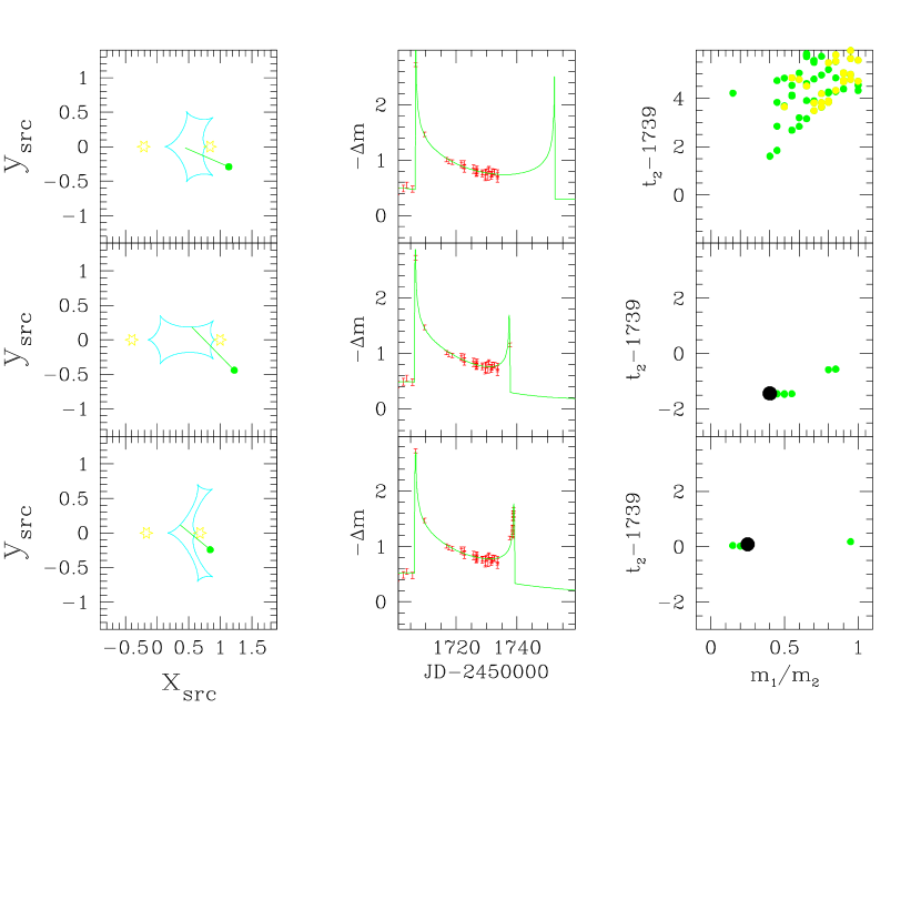
For the model fitting we discard the data from previous seasons as already used in the estimate. We use only measurements starting from the point, when magnification exceeds , since the details of the binary lens model have little influence on the low magnification tails of the light curve. We make numerical experiments for 2000-BUL-38 using data accumulated before: , , or . (These Julian dates correspond to nights six, two, and one day before the actual second caustic crossing). The first data sample constrains the models very weakly. Various intermediate separation binaries with full range of mass ratios as well as some close binaries with low mass ratio give acceptable fits to the observations. The second caustic crossing time can not be predicted: the value of this parameter corresponding to different acceptable models has a large spread; all acceptable models give too late . The geometry of the source - binary encounter, the light curve for the best model and the predicted time of the second crossing based on the first considered data sample are shown in the upper row of panels in Fig. 1.
The second data sample has only one extra point – the single observation made after three nights of no data. All acceptable models have intermediate separation and mass ratio . The predicted second crossing time is either one or two nights too early. (Compare the middle row in Fig. 1.)
Finally we use the data sample including the night preceding the second caustic crossing. The best model is marginally consistent with the data. Even the models with much higher all predict the time of the second crossing correctly. (See Fig. 1.)
The inspection of Fig. 1 shows that the “best” models chosen by our procedures based on different amount of data are not the same. One may think that the accumulation of the data can only serve as to reject some of the models, so the latest fits should be present among the earlier results. To clarify this point we take of our lowest fits obtained on the latest day considered, remove the observations of the previous night and refine the fits allowing for small changes in the encounter geometry, source size, and timing. The parameter which changes most appreciably during the refinement is the time of the second crossing; for all models considered its value decreases and becomes day too early. The single observation of remains on the growing part of the light curve. (The jump to the other side of the caustic is not excluded by the refinement procedure, but the placing of the observation point on steeply falling part of the theoretical light curve has low probability.) The models selected by the fits to the data sample and then fitted to data sample remain (after refinement) significantly worse than the models selected from the beginning with the fits to data sample. This shows that the model preferred by the data may change when the data is accumulated.
4.2 2000-BUL-46
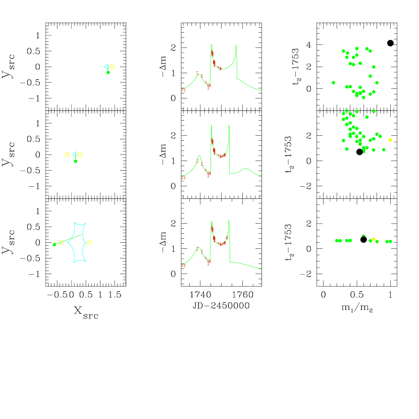
We treat this event with a manner similar to 2000-BUL-38. We adjust the errors using a much lower factor (). We consider three data samples accumulated before , , or , which correspond to observations made four, two, or one day before the caustic crossing. Because the event begins with the source passing close to the cusp and then through the caustic, the models are better constrained than for the other event considered. The first data sample can be fitted by models representing the three families of binary lenses (close, intermediate, and wide). The fits are marginally consistent with the data. The best model is a wide binary. Predicted crossing times are from one day too early to four days too late. (Compare Fig.2.) The marginal fits to the second data sample are similarly distributed in the plane of physical binary parameters . A close binary with the correct prediction of the crossing gives the best fit now, but other marginally consistent models give crossings up to four days too late. The last data sample leaves us only with intermediate and wide binaries, and the best model belongs to the former class. All the marginally consistent models give the right crossing time within accuracy of , except one, for which the prediction is too late.
4.3 Fitting “square root” formula
For comparison we use a method which can only be applicable to the part of the data representing flux increase toward the caustic. For a point source close to the crossing one can use a generic form of the light curve given by the formula:
| (10) |
There are three unknown parameters: the flux measured shortly after the crossing , a constant , which is proportional to of eq. (7), and the time of the crossing . Having three exact measurements of the flux in the region of formula validity, one would be able to calculate the time of the crossing. For any three points representing monotonically increasing flux, such that the middle point is below the straight line joining the other two points, the fit of the above formula is possible and gives some . Since the actual light curve is not well approximated by the formula far from the crossing or very close to the crossing, when the limited size of the source becomes important, one expects quite large scatter in fitted values of . We simulate the process of applying such a procedure.
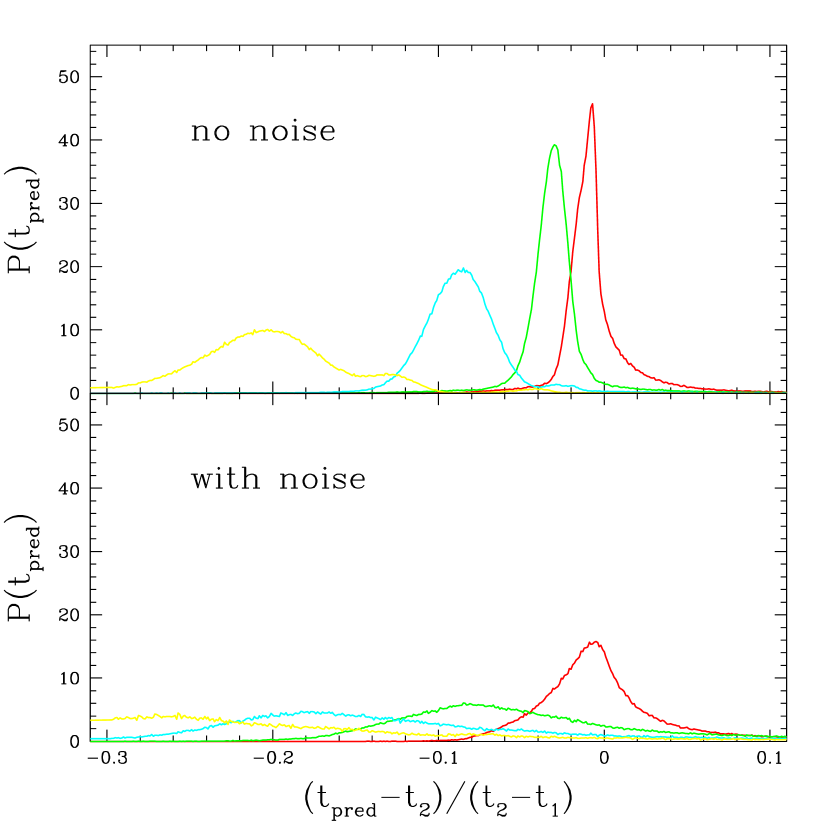
We use models with broad distribution of separations () and mass ratios (). For each model we draw at random source paths crossing caustics, with different directions and encounter parameters. For each path we find and - the positions of crossings along the source trajectory, and - at the magnification minimum. We use sources substantially (20 to 100 times) smaller than the distance between caustic crossings - otherwise the “U-shape” of the light curve would not be very pronounced. We divide the path between and into six equal sections and draw randomly “points of observations” from each of them, calculating also the corresponding magnifications. For any three points belonging to three consecutive sections we fit our formula and find the predicted time of the crossing . The distributions of predictions made this way are shown in the upper panel of Fig. 3. Different curves correspond to fits based on points drawn from different fragments of the source trajectory. The predictions become more accurate and less scattered, when one uses observations closer to the crossing, as expected. All the predictions are systematically shifted toward “too early”. In the lower panel we show the results of a similar procedure but each “observation” has now “measurement error” included. (Errors in stellar magnitudes are modeled as Gaussian with , typical for microlensing observations.) The observational noise introduces an extra scatter to the predictions, which also become more biased. Applying the method to a larger number of observation points would effectively diminish the noise and give results intermediate between those shown in the upper and lower panels.
We apply the light curve fit based on eq. (10) to real data for BUL-38 and BUL-46. Again, as in the case of fitting binary lens models, we choose various data subsamples each containing points, this time using only the observations obtained when the source was brightening toward the second caustic crossing. For these particular events the sensible fits are possible only late, at most two nights before the crossing, and only the predictions on the last day are correct. (In the case of BUL-38 the fit based on data terminating two days before the crossing gives a too early prediction, probably due to the large error in the single point of the night . In the case of BUL-46 the data terminating on leads to a fit with very broad minimum, allowing for crossing between and .) One can see again, that correct prediction of the second caustic crossing can only be made very late.
5 DISCUSSIONS
We have tried to fit binary lens models to the light curves representing caustic crossing events using incomplete data. Our purpose is to check whether it is possible to predict the night of the second caustic crossing and if this is the case, how early the reasonable prediction can be made. The answer we obtained is not very promising: in the two cases considered the unambiguous predictions could only be made based on the data including the observations from the last night before the crossing. These “late” predictions are true in the sense that they agree with the complete data sets for the events considered. The predictions made earlier are unreliable since they give unacceptably large spread in the time of the second crossing.
The simplified approach using the square root formula is much less time consuming but is also unable to give a reasonable early prediction of the second crossing of the caustic. Our simulations of such approach are too simplified: the application to the real data gives worse predictions than expected, probably due to the uneven time distribution of observations.
The example of 2000-BUL-38 shows that the uneven coverage of the light curve, especially the situation when the last observation used in fitting is separated from the earlier data may strongly bias the predictions. The extrapolation is always strongly dependent on the last known data point, so it is important to have this point measured accurately. Having more than one data point per night certainly improves the situation. On the other hand the models one gets from the fitting procedure depend on the particular data sets and their errors, so the predictions biased either way are probably unavoidable.
The fact that the binary lens models are not well constrained is known from the papers devoted to the subject (see in particular Dominik 1999; Albrow et al. 1999b). The models giving acceptable fits to the given light curves belong to the quite large regions in the plane. Our study shows that the regions of acceptable models can have either broad or narrow spread in the second caustic crossing time, depending on the chosen subsample of data used in the fit. On the other hand it is well known that the full coverage of the crossing is sufficient to obtain a precise estimate of its time, regardless of the lens model. Our estimates seem to converge to the right solution, but slowly.
In our approach we have neglected completely the possible motion of the binary system. The inclusion of the binary rotation may improve the fit since it offers more parameters to the model (e.g. Afonso et al. 200). Since our models are weakly constrained, at least for the data samples considered, we do not expect extra parameters to improve the situation. Similarly, without well sampled caustic crossing we do not attempt to fit the limb darkening parameter. We use an ad hoc method for the initial guess of the source size. We allow for the limited changes in this parameter during the refinement of our models. Since the refinement procedure is applied only to a limited number of candidate models chosen on the basis of the approximate value, and the allowed variation of the parameters on each step is very limited, we can not claim that our models are optimized for the source size to the same extent as for other parameters. Comparing the source radii of our best models for different data sets with the radii obtained with the fits to the second caustic crossings, we see the agreement between them up to a factor two.
Our simulations show, that the early predictions of the expected time for the second caustic crossing are not possible. The predictions become reliable only very shortly before the caustic crossing. The safest observational strategy is then to sample as densely as possible once a binary light curve starts to rise from the inter-caustic minimum.
Acknowledgments
We thank Bohdan Paczyński for encouragements and helpful discussions. This work would not be possible without the data released in real-time by the OGLE collaboration. This work was supported in part by the NSF grant AST 98-20314 and the Polish KBN grant 2-P03D-01316.
References
- [1] Afonso C., Alard C. Albert J.N. et al., 2000, ApJ, 532, 340
- [2] Alcock C. et al., 2000a, ApJ, 541, 270
- [3] Alcock C. et al., 2000b, ApJ, 541, 734
- [4] Alcock C. et al., 2000c, ApJ, 542, 257
- [5] Alcock C. et al., 2000d, ApJ, 542, 281
- [6] Alcock C. et al., 2000e, astro-ph/0011506
- [7] Albrow M.D. et al., 1999a, ApJ, 522, 1011
- [8] Albrow M.D. et al., 1999b, ApJ, 522, 1022
- [9] Beaulieu J.-P. & Marquette J.-B., 2000, in: IAU Colloquium No 176, L. Szabados and D. Kurtz eds., p.139-144
- [10] Dominik M. 1998, A&A, 333, L79
- [11] Dominik M. 1999, A&A, 341, 943
- [12] Gould A. Gaucherel C. 1997, ApJ, 477, 580
- [13] Heyrovski D., Sasselov D., Loeb A., 2000 ApJ, 543, 406
- [14] Lasserre T. et al., 2000, A&A, L39
- [15] Lennon D.J., Mao S, Fuhrmann K. Gehren T. 1996, ApJ, 471, L23
- [16] Lennon D.J., Mao S., Reetz J., Gehren T., Yan L., Renzini A. 1997, the Messenger, 90, 30
- [17] Mao S., 1999, in: “Gravitational Microlensing: Recent Progress and Future Goals”, ed. T.G. Brainerd & C.S. Kochanek, Boston University
- [18] Mao S. & Paczyński B., 1991, ApJ, 374, L37
- [19] Mao S. & Di Stefano R. 1995, ApJ, 440, 22
- [20] Mao S. & Loeb A. 2001, ApJ, 547, L97
- [21] Minnitt D., Vandehei T., Cook K.H., Griest K., Alcock C., 1998, ApJ, 499, L175
- [22] Paczyński B. 1986, ApJ, 304, 1
- [23] Paczyński B. 1996, A.R.A.&A., 34, 419
- [24] Press W. H., Teukolsky S. A., Vetterling W. T., & Flannery B. P. 1992, Numerical Recipes in Fortran (NY: CUP), p. 367
- [25] Sahu K., Sahu M. S. 1998, ApJ, 508, L147
- [26] Szymański M. et al., 2000, Astronomische Gesellschaft Meeting Abstracts, 16, 19
- [27] Udalski A., Kubiak M., & Szymański M., 1997, Acta Astron., 47, 319
- [28] Udalski A., Szymański M., Kaluzny J., Kubiak M., Mateo M., Krzemiński W., & Paczyński, B., 1994a, Acta Astron., 44, 227
- [29] Udalski A., Szymański M., Mao S., di Stefano R., Kaluzny J., Kubiak M., Mateo M., & Krzemiński, W., 1994b, ApJ, 436, L103
- [30] Udalski, A., Szymański, M., Stanek, K. Z., Kaluzny, J., Kubiak, M., Mateo, M., Krzemiński, W.; Paczyński, B., & Venkat, R., 1994c, Acta Astron, 44, 165
- [31] Udalski A., Żebruń K., Szymański M., Kubiak M., Pietrzyński G., Soszyński I., & Woźniak P., 2000, Acta Astron., 50, 1
- [32] Witt H.J., 1990, A&A, 236, 311
- [33] Witt H.J., Mao S., 1995, ApJ, 447, L105
- [34] Woźniak P., 2000, astro-ph/0012143
- [35] Woźniak P., 2001, in preparation