Light Curves from an Expanding Relativistic Jet

Abstract

We perform fully relativistic hydrodynamic simulations of the deceleration and lateral expansion of a relativistic jet as it expands into an ambient medium. The hydrodynamic calculations use a 2D adaptive mesh refinement (AMR) code, which provides adequate resolution of the thin shell of matter behind the shock. We find that the sideways propagation is different than predicted by simple analytic models. The physical conditions at the sides of the jet are found to be significantly different than at the front of the jet, and most of the emission occurs within the initial opening angle of the jet. The light curves, as seen by observers at different viewing angles with respect to the jet axis, are then calculated assuming synchrotron emission. For an observer along the jet axis, we find a sharp achromatic ‘jet break’ in the light curve at frequencies above the typical synchrotron frequency, at $t_{jet}\approx 5.8(E_{52}/n_{1})^{1/3}(\theta_{0}/0.2)^{8/3}$ days, while the temporal decay index $\alpha$ ($F_{\nu}\propto t^{\alpha}$) after the break is steeper than $-p$ ($\alpha=-2.85$ for $p=2.5$). At larger viewing angles $t_{jet}$ increases and the jet break becomes smoother.

1 The Hydrodynamics

The hydrodynamic simulations are performed using a fully relativistic 2D AMR code. The jet propagates into a cold and homogeneous ambient medium of number density $n_{1}\ {\rm cm}^{-3}$. We use $n_{1}=1$, typical of the ISM. We assume an adiabatic evolution (i.e. that radiation losses do not influence the dynamics). For the initial conditions, we use a wedge of opening angle $\theta_{0}=0.2$ taken out of the Blandford McKee BM self similar spherical solution, with an isotropic equivalent energy of $E_{52}10^{52}$ ergs, where we use $E_{52}=1$. Since the lateral expansion is expected to become significant only when the Lorentz factor of the flow drops to $\gamma\sim 1/\theta_{0}=5$, the initial Lorentz factor of the shock was chosen to be $\Gamma=\sqrt{2}\gamma=23.7$.

Figure (1) shows a 3D view of the jet at the last time step of the simulation, with color-maps of the proper number density, $n^{\prime}$, and proper emissivity. Primed quantities are measured in the local rest frame of the fluid. While the number density does not change significantly between the front and the sides of the jet, the emissivity is significant only at the front of the jet, and drops sharply at angles larger than the initial opening angle, $\theta_{0}$. The overall egg-shaped structure is very different from the quasi-spherical structure assumed in 1D analytic models.

2 The Light Curves

The synchrotron spectral emissivity, $P^{\prime}_{\nu^{\prime}}$, is calculated using the physical conditions determined by the hydrodynamic simulation. The electrons and the magnetic field are assumed to hold fractions $\epsilon_{e}$ and $\epsilon_{B}$, respectively, of the internal energy density, $e^{\prime}$, while the electrons posses a power law energy distribution, $N(\gamma_{e})\propto\gamma_{e}^{-p}$ for $\gamma_{e}>\gamma_{m}=\left[(p-2)/(p-1)\right](\epsilon_{e}e^{\prime}/n^{\prime}m_{e}c^{2})$. For simplicity, we ignore the effects of electron cooling and self absorption, so that $P^{\prime}_{\nu^{\prime}}\propto\nu^{\prime 1/3}$ for $\nu^{\prime}<\nu^{\prime}_{m}$ and $P^{\prime}_{\nu^{\prime}}\propto\nu^{\prime(1-p)/2}$ for $\nu^{\prime}>\nu^{\prime}_{m}$, where $\nu^{\prime}_{m}$ is the local synchrotron frequency of an electron with $\gamma_{e}=\gamma_{m}$; $F_{\nu}$ is calculated using the formalism of GPS , summing over the contributions from the finite 4-volume of the simulation.

Figure (2) shows the radio light curves seen by an observer along the jet axis ($\theta_{obs}=0$). For simplicity, cosmological corrections are not included. The insert shows an optical light curve as seen by observers at three different viewing angles with respect to the jet axis: $\theta_{obs}/\theta_{0}=0,1,2$. We obtain an achromatic ‘jet break’ in the light curve for $\nu>\nu_{m}(t_{jet})$ (as predicted by simple semi-analytic models Rhoads ; SPH ) at $t_{jet}(\theta_{obs})$, where $0.66t_{jet}(\theta_{0})\approx t_{jet}(0)\approx 5.8(E_{52}/n_{1})^{1/3}(\theta_{0}/0.2)^{8/3}$ days. Defining $\alpha$, $\beta$ by $F_{\nu}\propto\nu^{\beta}t^{\alpha}$, the shape of the break may be approximated by

$$F_{\nu}=F_{0}\nu^{\beta}\left[(t/t_{jet})^{-s\alpha_{1}}+(t/t_{jet})^{-s\alpha_{2}}\right]^{-1/s}\ ,$$ (1)

where $\alpha_{1}=\alpha(t\ll t_{jet})$, $\alpha_{2}=\alpha(t\gg t_{jet})$ and the parameter $s(\theta_{obs})$ determines the sharpness of the break, and ranges between $s(\theta_{0})\approx 1$ to $s(0)\approx 4.5$, indicating that the break is sharper at smaller $\theta_{obs}$. For $\nu<\nu_{m}(t_{jet})$, there is only a moderate and more gradual change in $\alpha$, until the time when $\nu_{m}=\nu$. For $\nu>\nu_{m}$ we find that $\alpha_{2}$ is slightly smaller than $-p$ (the value predicted by most simple models) for $\theta_{obs}=0$ ($\alpha_{2}=-2.85$ for $p=2.5$).

3 Discussion

We find that the physical conditions at the sides of the jet are significantly different than at the front of the jet, and most of the radiation is emitted within the initial opening angle of the jet [$\theta<\theta_{0}$; see Figure (1)]. Therefore, the frequently used assumption of a homogeneous jet seems inadequate. For $\nu>\nu_{m}(t_{jet})$ we find a sharp achromatic break in the light curve at $t_{jet}=5.8(E_{52}/n_{1})^{1/3}(\theta_{0}/0.2)^{8/3}$ days, for $\theta_{obs}=0$, while at larger viewing angles $t_{jet}$ increases and the break becomes smoother. For $\nu<\nu_{m}(t_{jet})$ the change in the temporal index $\alpha$ near $t_{jet}$ is more moderate and gradual. The value of $\alpha$ for $t>t_{jet}$, $\nu>\nu_{m}$, $\theta_{obs}=0$ is slightly smaller than $-p$ ($\alpha=-2.85$ for $p=2.5$). Finally, we note that $t_{jet}(\theta_{obs}=\theta_{0})\approx 1.5t_{jet}(\theta_{obs}=0)$. Since, in order to detect a burst in $\gamma$-rays we require that $\theta_{obs}\mathrel{\hbox{\hbox to0.0pt{\hbox{\lower 4.0pt\hbox{$\sim$}}\hss}\hbox{$<$}}}\theta_{0}$, this may induce an uncertainty of up to $15\%$ when deducing the value of $\theta_{0}$ from $t_{jet}$, unless $\theta_{obs}$ is well constrained.

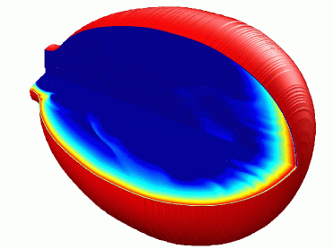
Figure 1: A 3D view of the jet at the last time step of the simulation. The outer surface represents the shock front while the two inner faces show the proper number density (lower face) and proper emissivity (upper face) in a logarithmic color scale

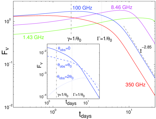
Figure 2: Radio light curves (flux density, $F_{\nu}$, in arbitrary units, as a function of the observed time in days) for an observer along the jet axis. We use $\epsilon_{e}=\epsilon_{B}=0.1$, $p=2.5$. The observed times, for an observer along the jet axis, when the Lorentz factors $\gamma$ of the shocked fluid (vertical dash-dotted line) or $\Gamma$ of the shock (vertical dotted line) drop to $1/\theta_{0}$, for an extrapolated spherical evolution, are indicated. (insert) Optical light curves for observers at viewing angles $\theta_{obs}/\theta_{0}=0,1,2$ with respect to the jet axis.

References

(1) R.D. Blandford, C. F. McKee: Phys. of fluids, 19,
1130 (1976)
(2) J. Granot, T. Piran, R. Sari: ApJ, 513, 679 (1999)
(3) J.E. Rhoads: ApJ, 525, 737 (1999)
(4) R. Sari, T. Piran, T. Halpern: ApJ, 519, L17 (1999)