The Nearest Neighbor Alignment of Cluster X-ray Isophotes

Abstract

We examine the orientations of rich galaxy cluster X-ray isophotes with respect to their rich nearest neighbors using existing samples of Abell cluster position angles measured from Einstein and ROSAT observations. We study a merged subset of these samples using updated and improved positions and redshifts for Abell/ACO clusters. We find high confidence for alignment, which increases as nearest neighbor distance is restricted. We conclude that there is a strong alignment signal in all this data, consistent with gravitational instability acting on Gaussian perturbations.

1 Introduction

A conventional picture suggests that galaxy clusters form by hierarchical clustering whereby material (gas, galaxies etc.) flows into denser regions along interconnecting large-scale filamentary structures (Shandarin & Klypin 1984). As a result of this infall, clusters, in both optical and X-ray, appear aligned with their neighbors, especially when members of the same supercluster. Observationally, this picture has been supported by previous alignment studies (see below), and dynamical evidence of relic drainage along supercluster filaments (Novikov et al. 1999).

Most numerical simulations of structure formation by gravitational instability acting on Gaussian initial perturbations predict cluster alignment on some scale (e.g. Splinter et al. 1997; Onuora & Thomas 2000). These simulations show that cluster alignments are not crucial for discriminating between cosmological models, but they support the gravitational instability hypothesis of structure formation.

1.1 Optical Alignments

The projected shapes of galaxy clusters on the sky are often elongated images (Carter & Metcalfe 1980) which can be approximated as ellipses. The major axes of these define projected position angles, measured counter-clockwise from north. Binggeli (1982) found that the major axes of galaxy clusters tend to point toward their nearest neighbor. Since then there have been many optical studies of cluster alignments. Most of the literature finds alignment on some scale. For example, Flin (1987) and Rhee & Katgert (1987) found significant nearest neighbor alignment for separations, d_n $<$ 30 h^-1Mpc. West (1989) found that clusters which reside within the same supercluster are significantly aligned on scales of 30 h^-1Mpc and possibly out to 60 h^-1Mpc. Rhee, van Haarlem & Katgert (1992) also detected alignment for clusters within the same supercluster, but they did not find significance for nearest neighbor alignment. Plionis (1994) found significant alignment for d_n $<$ 30 h^-1Mpc, with weaker signals for larger separations up to 60 h^-1Mpc. On the other hand, Strubles & Peebles (1985) did not detect a significant alignment signal (however, see Argyles et al. 1986).

1.2 X-ray Alignments

Individual galaxies may not be the best tracers of the shape of a cluster. Problems can arise from foreground/background contamination, as well as the contribution of a discrete noise term. However, it is believed that the X-ray emitting gas within a cluster traces its gravitational potential (Sarazin 1986). X-ray morphology is, then, probably the best observable for determining galaxy cluster shape and orientation. Likewise, since optical alignment has been measured and is well supported, X-ray isophotal alignment is crucial for understanding nearest neighbor cluster alignment.

Unfortunately there have not been many X-ray alignment studies. Ulmer, McMillan, & Kowalski (1989–hereafter UMK) performed the first alignment study using Einstein data on 46 clusters and found no significant result. However, Chambers, Melott, and Miller (2000–hereafter CMM) recently re-examined the UMK results using updated cluster positions and found a very strong signal. Rhee, van Haarlem & Katgert (RvHK 1992) used the X-ray images of clusters in a study of supercluster member alignment. They examined clusters within the same supercluster and a significant signal for nearest neighbor alignment was not detected. However, West (1989) convolved X-ray and optical data to find that clusters are aligned when they are members of the same supercluster. Further, West, Jones & Forman (1995) showed that the X-ray substructure within clusters tends to share the orientation with its local environment out to 10$h^{-1}$Mpc. Of the above analyses, which all used Einstein X-ray imagery, only UMK and RvHK did nearest neighbor alignment studies, and neither found support for the hypothesis. However, CMM, West, and West, Jones and Forman find support for the hypothesis that the shapes of galaxy clusters are aligned with LSS environment (as traced by nearest neighbors). The amount and quality of X-ray cluster data since the UMK and RvHK analyses, along with the conflicting reports discussed above, prompts a new analysis of the nearest neighbor cluster alignment with X-ray isophotes.

In this paper we present cluster alignment results for three samples with previously determined projected position angles. We merge and filter these to obtain a larger sample. Our goal is to use a well-controlled sample to test whether the X-ray emitting gas within rich clusters is aligned with its nearest neighboring rich cluster. One of our adopted samples was previously tested for nearest neighbor alignment in cases where clusters were within the same supercluster; a significant signal was not detected (RvHK, see above). The other samples we adopt have not been tested for nearest neighbor alignment (Mohr, Evrard, Fabricant & Geller 1996; Kolokotronis, Basilakos, Plionis & Georgantopoulos 2001). In an earlier work (CMM), we studied a subsample of cluster orientations previously examined by UMK. Although they did not find a signal for nonuniform orientations, we detected a significant signal for alignment by using the Wilcoxon rank-sum test (WRS; Lehmann 1975). As the WRS is more effective in testing for alignments, we use it in the present study. We use q_o = 0 and h = 100H_o km s^-1 Mpc^-1 throughout.

2 Data and Analysis

2.1 The Cluster Samples

We did a literature search for existing X-ray position angles. Rhee, van Haarlem & Katgert used 107 rich clusters of galaxies to study alignments within superclusters. Of these, 27 had X-ray position angles determined from Einstein imagery (Rhee & Latour 1991). When assigning these angles, they focused on the entire X-ray image within the largest circular region centered on the peak of the X-ray emission. Although significant alignment was detected for clusters within the same supercluster, nearest neighbor alignment was not found. We therefore adopt these 27 RvHK clusters as one of our samples. Position angles found from a moments method and an inertia tensor method are both available; we use the latter in this analysis.

Mohr, Evrard, Fabricant & Geller (1996–MEFG hereafter) used a sample of 65 galaxy clusters observed by the Einstein IPC to constrain the range of cluster X-ray morphologies. The core of the X-ray emission was emphasized in their analysis. Emission-weighted cluster orientations were calculated from the Fourier expansion of the photon distribution. In the present work we only use Abell clusters for which we have accurate redshift information. This leaves 54 MEFG clusters (see next section).

Kolokotronis, Basilakos, Plionis & Georgantopoulos (2001–KBPG hereafter) found significant correlations between the Abell-APM optical and ROSAT X-ray shape parameters of 22 rich galaxy clusters. They concluded that the dynamical state of clusters can be indicated by either part of the spectrum. Their X-ray analysis focuses on the inner region of the emission. Position angles were calculated by an inertia tensor method. We also use this sample of 22 KBPG clusters.

2.2 Nearest Neighbor Sample

We measure the nearest neighbor distances using rich ($R\geq 1$) clusters from the Abell (1958) and Abell, Corwin, and Olowin (1989) catalogs. To have a well controlled neighbor sample, we follow the strategy of CMM. As R=0 clusters are not part of Abell’s statistical sample, we only use R $\geq$ 1 clusters in our study. Also, since more accurate redshifts are now available, we have updated the redshifts of all clusters. The redshifts and coordinates used are mainly from the MX Northern Abell Cluster Survey (MX; Slinglend et al. 1998; Miller et al. 2001) and the ESO Nearby Abell Cluster Survey (Katgert et al. 1996). We use the richness values from the Abell catalog for the Abell/ACO overlap region ($-27^{\circ}\leq\delta\leq-17^{\circ}$). There are 336 rich (R $\geq$ 1) clusters within the $|$b$|$ $\geq$ 30^o and 0.012 $\leq$ z $\leq$ 0.10 boundary of this survey. These clusters have on average 25 redshifts per cluster and 86% have at least two measured galaxy redshifts.

We search through the 336 rich clusters for possible nearest neighbors. We note that there are not many clusters with d_n $>$ 30h^-1Mpc. A potential weakness of most previous nearest neighbor studies is the neglect of the survey boundary location. Therefore, we note the distance and direction to the neighbor, and the distance to the boundary of the survey, all with respect to the subject cluster. Since a potential nearest neighbor may be hidden just outside the boundary, we disqualify any pair in which the distance to the boundary was less than the distance to the nearest neighbor.

We would like to briefly discuss the advantages of our controlled samples. By using $R\geq 1$ clusters, we are ensured that we have a statistically complete subsample. Miller et al. (1999) found that cluster mean redshifts based on only one galaxy redshift are often erroneous by $\sim$ 5 h^-1Mpc, which can throw off the distance to the nearest neighbor and perhaps more importantly, the identification and direction to the true nearest neighbor. Thus, updating the cluster redshifts makes sure that we are using the correct nearest neighbor (and nearest neighbor distance). And finally, excluding cases where the boundary distance is closer than the neighbor also helps to prevent the identification of an incorrect nearest neighbor.

2.3 Statistical Samples

After we apply these stringent criteria to our data, we are left with three subsamples. Twenty seven of the RvHK clusters are rich and within the boundary of the survey. However, in four cases, the boundary was closer than the nearest neighbor, leaving 23 RvHK clusters. The sample of MEFG lost 25 clusters because of richness or not being within the survey volume. Of the 29 remaining, six pairs did not obey our nearest neighbor-boundary distance requirement. We therefore can use 23 MEFG clusters. Four of the original KBPG clusters did not obey the richness and boundary criteria. And five of the 18 remaining clusters had the boundary distance closer than the neighbor. That is, we have 13 KBPG clusters after our cuts. In summary, our statistical subsamples for RvHK, MEFG and KBPG contain 23/27, 23/54 and 13/22 clusters, respectively – see Table 2.

We merged these three subsamples to obtain a final controlled sample. We start with the 59 objects in our subsamples. Some clusters appear in more than one subsample, so there are actually 48 individual Abell clusters total. That is, there are 11 Abell clusters with two independently measured orientations. Nine of these clusters are common to the MEFG and RvHK samples and the other two Abell clusters are in both MEFG and KBPG. We have kept eight (1367, 1650, 1983, 2065, 2147, 2199, 3158 & 3266) out of these 11 clusters, discarding three (1767, 2124 & 2151) because of inconsistent orientations. We define consistent orientations are $\Delta$$\theta$ $\leq$ 25^o. The position angles of the eight consistent clusters were tested and found to be highly correlated. Thus, which of these position angle we choose to use should not effect our results. We alternately pick position angles by chronology in Abell number, keeping three RvHK, three MEFG and the two KBPG. This makes a total of 45 total clusters in our final merged sample. We have verified that different choices for these eight clusters does not significantly change our conclusions.

2.4 Analysis

We use published position angles, $\theta$, measured counter-clockwise from north, for our statistical samples. The absolute value of the projected angular difference between this angle and the direction to the nearest neighbor defines the pointing angle, $\phi_{p}$, 0^o $\leq$ $|\phi_{p}|$ $\leq$ 90^o.

We define alignment as the tendency for the pointing angles, $|\phi_{p}|$, to be systematically smaller than they would be if distributed isotropically over this interval. The Wilcoxon rank-sum test (WRS; Lehmann 1975) tests for this. The null hypothesis of WRS is that the sample is not systematically smaller or larger than the (uniform) parent population. It has been common for the Kolmogorov-Smirnov (KS) test to be used in alignment studies. However, KS tests for any difference from the assumed parent population, in this case a pointing angle distribution uniform over its possible range. For example, KS would show a signal if there were an excess of angles at 45^o, but this is not alignment (systematically small angles). By being sensitive to any deviation, KS has reduced sensitivity to the particular deviation for which we are testing. WRS, on the other hand, places the angles in the test sample in rank order against the angles in the parent population (comparison sample). Examination of these ranks allows a specific test for whether the sample tends to be significantly larger or smaller.

We have run the WRS test twice on each data sample. The first, which we call ”uniform”, uses a control group placed at equal intervals between 0^o and 90^o with a mean of 45^o. In the second method, called ”remix”, the control is constructed by reassigning cluster position angles randomly within the sample, and new pointing angles constructed using these. The purpose of this second method is to detect any possible systematic preference for a given angle as a source of alignment. Of course, larger fluctuations (by $\sqrt[]{2}$) are expected using this method. We show the average of five remix computations. The difference between the remix and uniform methods is barely more than 1$\sigma$ for this size remix population.

Table 1 shows the results of WRS on the merged and re-mixed samples. We have included D_max, the number of clusters, N_cl within D_max, and the probability that the alignment could have arisen as a random sample of the control parent population.

We tested our merged sample for nearest neighbor alignment at various maximum nearest neighbor distances, D_max. When D_max $\geq 30$ h^-1Mpc signals for alignment are low. However, restricting D_max $\leq 20$ h^-1Mpc, we find a significant signal for alignment with a 1.26% probability for no alignment. The maximum signal for alignment occurs at D_max $\leq 10$ h^-1Mpc where the probability for no alignment is only 0.18%.

3 Conclusion and Discussion

We tested three samples of previously determined X-ray position angles, 45 clusters total, for nearest neighbor alignment. We found, using the Wilcoxon rank-sum (WRS) test, that the X-ray isophotes in our samples are aligned with their nearest neighboring rich Abell cluster, consistent with the gravitational instability hypothesis (Shandarin & Klypin 1984). Alignment significantly increases as the maximum neighbor distance is decreased. In fact, we noticed a transition zone, before which isophotal alignment becomes significant. Our data shows that the orientation of the X-ray emitting gas within rich clusters is correlated with nearest rich neighbor positions when d_n $\leq$ 20 h^-1Mpc; this distance roughly marks a transition zone from orientations being random to aligned. This transition distance is the same found by Novikov, et al. (1999) for alignment between cluster winds and the neighboring cluster population. It likely represents the wavelength undergoing collapse at this time in cosmic history, the so-called “pancaking scale” (Melott & Shandarin 1993; Shandarin et al. 1995).

Previously, Rhee, van Haarlem and Katgert had not detected nearest neighbor alignment in their sample which we adopted. If alignment were not present in our subset of 23 RvHK clusters, then this would work against our signal for alignment - especially since this is such a large fraction of our merged sample. However, we do not see this. Instead, we find a fairly significant signal in our data. We therefore speculate that updated positions and redshifts, as well as using a more controlled sample, (particularly our boundary distance condition) allowed us to get a signal for alignment from the RvHK data. In a previous work (CMM 2000) we also showed the X-ray data of Ulmer, McMillan and Kowalski (UMK 1989) exhibits alignment, contrary to their conclusions. Using a consistent data analysis and a clear statistical methodology, we have removed two crucial discrepancies from X-ray alignment studies; now, all samples tested (to our knowledge) have been shown to exhibit (or contribute to) significant X-ray alignment on similar scales.

4 Acknowledgments

ALM and SWC are grateful for financial support under NSF grant AST-0070702 and computing resources from the National Center for Supercomputing Applications.

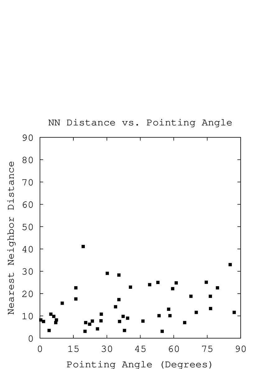
Figure 1: The distribution of pointing angle against nearest neighbor distance is shown for our 45 clusters in our merged sample. Pointing angles are generally $<$ 45^o for separations $<$ 20 h${}^{-1}Mpc$.

Table 1: WRS Results for the Statistical Samples

		Uniform	Remix
Dmax	Ncl	Prob.	Prob.
($h^{-1}$Mpc)		%	%
10	18	0.18	0.99
20	32	1.26	1.66
30	43	7.36	6.55
40	44	10.75	9.51

Table 2: Cluster Information

Source	Abell	z	$\theta$	NN Abell	z	$d_{n}$	$\phi$
MFEG	85	0.0556	169.0	87	0.0543	4.2	25.8
MFEG	119	0.0444	2.0	168	0.0448	11.6	70.1
MFEG	168	0.0448	165.0	119	0.0444	11.6	87.1
MFEG	399	0.0722	16.0	401	0.0748	8.2	7.4
MFEG	401	0.0748	23.0	399	0.0722	8.2	0.4
KBPG	500	0.0666	162.3	514	0.0720	18.8	67.7
KBPG	514	0.0720	126.8	500	0.0666	18.8	76.4
RvHK	1185	0.0326	99.0	1228	0.0352	13.3	76.5
RvHK	1291	0.0530	62.0	1377	0.0514	7.5	35.7
MFEG	1367	0.0214	145.0	1656	0.0231	22.6	79.6
RvHK	1367	0.0214	147.0	1656	0.0231	22.6	81.6
RvHK	1377	0.0514	96.0	1291	0.0530	7.5	1.6
MFEG	1644	0.0474	69.0	3555	0.0494	33.0	85.3
MFEG	1650	0.0845	174.0	1663	0.0827	7.7	46.2
RvHK	1650	0.0845	174.0	1663	0.0827	7.7	46.2
MFEG	1656	0.0231	80.0	1367	0.0214	22.6	16.1
MFEG	1767	0.0701	24.0	1904	0.0708	46.4	52.7
RvHK	1767	0.0701	125.0	1904	0.0708	46.4	26.3
MFEG	1775	0.0696	123.0	1795	0.0622	22.9	40.6
RvHK	1795	0.0622	19.0	1831	0.0613	9.0	39.3
RvHK	1809	0.0790	166.0	1780	0.0786	13.0	57.7
MFEG	1983	0.0449	111.0	2040	0.0457	25.0	42.0
RvHK	1983	0.0449	4.0	2040	0.0457	25.0	31.0
RvHK	1991	0.0579	179.0	1913	0.0528	25.1	74.6
RvHK	2029	0.0768	12.0	2028	0.0776	7.7	23.5
RvHK	2040	0.0457	25.0	1983	0.0449	25.0	52.9
RvHK	2063	0.0354	174.0	2147	0.0351	22.2	59.5
MFEG	2065	0.0723	153.0	2056	0.0746	7.8	27.4
RvHK	2065	0.0723	152.0	2056	0.0746	7.8	26.4
RvHK	2079	0.0656	170.0	2092	0.0670	9.8	37.3
RvHK	2092	0.0670	33.0	2079	0.0656	9.8	6.2
MFEG	2124	0.0654	177.0	2122	0.0663	2.7	51.7
RvHK	2124	0.0654	131.0	2122	0.0663	2.7	5.7
RvHK	2142	0.0899	147.0	2178	0.0928	29.1	30.2
MFEG	2147	0.0351	178.0	2151	0.0368	6.3	23.3
RvHK	2147	0.0351	179.0	2151	0.0368	6.3	22.3
MFEG	2151	0.0368	124.0	2152	0.0374	3.1	54.8
RvHK	2151	0.0368	102.0	2152	0.0374	3.1	76.8
RvHK	2152	0.0374	19.0	2151	0.0368	3.1	20.2
RvHK	2197	0.0308	173.0	2199	0.0299	3.5	4.1
MFEG	2199	0.0299	35.0	2197	0.0308	3.5	37.9
RvHK	2199	0.0299	35.0	2197	0.0308	3.5	37.9
MFEG	2410	0.0809	72.0	2377	0.0825	17.6	16.1
MFEG	2420	0.0848	61.0	2428	0.0846	14.1	33.9
MFEG	2657	0.0404	90.0	2506	0.0289	41.1	19.4
MFEG	2670	0.0759	130.0	2638	0.0825	24.8	61.1
KBPG	2717	0.0490	143.1	4059	0.0460	10.1	53.4
KBPG	2734	0.0620	7.8	2800	0.0640	24.0	49.2
KBPG	3093	0.0830	70.3	3111	0.0780	17.3	35.4
KBPG	3111	0.0780	28.3	3112	0.0750	10.8	27.5
KBPG	3112	0.0750	5.7	3111	0.0780	10.8	4.9
KBPG	3128	0.0600	53.8	3158	0.0602	7.0	64.9
KBPG	3158	0.0602	98.8	3128	0.0600	7.0	20.5
MFEG	3158	0.0602	108.0	3128	0.0600	7.0	11.3
KBPG	3223	0.0600	144.4	3151	0.0662	28.3	35.4
KBPG	3266	0.0605	45.8	3231	0.0570	15.7	10.0
MFEG	3266	0.0605	68.0	3231	0.0570	15.7	32.2
KBPG	3897	0.0698	93.3	2480	0.0710	7.0	7.1
KBPG	4059	0.0460	148.0	2717	0.0490	10.1	58.3

References

- (1) Abell, G.O., 1958, ApJS, 3, 211
- (2) Abell, G.O., Corwin Jr., H.G., Olowin, H.G., 1989, ApJS, 70, 1
- (3) Argyles, P.C., Groth, E.J., Peebles, P.J.E., Struble, M.F., 1986, ApJ, 91, 471
- (4) Binggeli, B., 1982, A&A, 107, 338
- (5) Carter, D., and Metcalfe, N., 1979, MNRAS, 191, 325
- (6) Chambers, S.W., Melott, A.L., Miller, C.J., 2000, ApJ, 544, 104
- (7) Flin P., 1987, MNRAS, 228, 941
- (8) Kolokotrinis, V., Basilakos, S., Plionis, M., Georgantopoulos, I., 2001, MNRAS, 320, 49
- (9) Katgert, P., et al. 1996, A&A, 310, 8
- (10) Lehmann, E.L., 1975 Nonparametrics: Statistical Methods Based on Ranks (Prentice Hall: New Jersey)
- (11) Melott, A.L., & Shandarin, S.F., 1993, ApJ, 410, 496
- (12) Miller, C.J., & Batuski, D., 2000, submitted to ApJ(astro-ph/0002295)
- (13) Miller, C.J., Batuski, D.J., Slinglend, K.A., and Hill, J.M. 1999 ApJ 523, 492
- (14) Miller, C.J., Krughoff, K.S., Batuski, D.J., Slinglend, K.A.,& Hill, J.M. 2000, submitted to AJ
- (15) Mohr, J.J, Evrard, A.E., Fabricant, D.G & Geller, M.J., 1995, ApJ, 447, 8
- (16) Novikov, D.I., Melott, A.L., Wilhite, B.B., Kauffman, M., Burns, J.O., Miller, C.J, and Batuski, D.J., 1999 MNRAS, 304, L5
- (17) Onuora, L.I., and Thomas, P.A., 2000 MNRAS, 319, 614
- (18) Plionis, M., 1994, ApJ 95, 401
- (19) Rhee, G.F.R.N., Katgert P., 1987, A&A, 183, 217
- (20) Rhee, G.F.R.N. & Latour, H.J., A&A, 243, 38
- (21) Rhee, G.F.R.N., van Haarlem M., Katgert P., 1992, AJ, 103, 1721
- (22) Sarazin, C.L., 1986, Rev. Mod. Phys., 58, 1
- (23) Shandarin, S.F., and Klypin, A.A., 1984, Sov Astron. 28, 491
- (24) Shandarin, S.F., Melott, A.L., McDavitt, K., Pauls, J.L., & Turner, J., 1995, Phys.Rev.L, 75, 7
- (25) Slinglend, K., Batuski, D., Miller, C., Haase, S., Michaud, K., & Hill, J. 1998, ApJS, 115, 1
- (26) Splinter, R.J., Melott A.L., Linn, A.M., Buck C., Tinker J., 1997, ApJ 479, 632
- (27) Strubles, M.F., Peebles, P.J.E., 1985, AJ, 90, 592
- (28) Ulmer, M.P., McMillan, S.L.W., Kowalski, M.P., 1989, ApJ, 338, 711
- (29) West, M.J., 1989, ApJ, 347, 610
- (30) West, M.J., Jones C., Forman, W., 1995, ApJ, 451, L5