100-year Mass Loss Modulations on the Asymptotic Giant Branch

Abstract

We analyze the differences in infrared circumstellar dust emission between oxygen rich Mira and non-Mira stars, and find that they are statistically significant. In particular, we find that these stars segregate in the K-[12] vs. [12]-[25] color-color diagram, and have distinct properties of the IRAS LRS spectra, including the peak position of the silicate emission feature. We show that the infrared emission from the majority of non-Mira stars cannot be explained within the context of standard steady-state outflow models.

The models can be altered to fit the data for non-Mira stars by postulating non-standard optical properties for silicate grains, or by assuming that the dust temperature at the inner envelope radius is significantly lower (300-400 K) than typical silicate grain condensation temperatures (800-1000 K). We argue that the latter is more probable and provide detailed model fits to the IRAS LRS spectra for 342 stars. These fits imply that 2/3 of non-Mira stars and 1/3 of Mira stars do not have hot dust ($>$ 500 K) in their envelopes.

The absence of hot dust can be interpreted as a recent (order of 100 yr) decrease in the mass-loss rate. The distribution of best-fit model parameters agrees with this interpretation and strongly suggests that the mass loss resumes on similar time scales. Such a possibility appears to be supported by a number of spatially resolved observations (e.g. recent HST images of the multiple shells in the Egg Nebula) and is consistent with new dynamical models for mass loss on the Asymptotic Giant Branch.

1 INTRODUCTION

Asymptotic Giant Branch (AGB) stars are surrounded by dusty shells which emit copious infrared radiation. Even before the IRAS data became available, it was shown that IR spectra of AGB stars can be reasonably well modeled by thermal emission from dust with radial density distribution $\propto r^{-2}$, and optical properties for either silicate, or carbonaceous grains (Rowan-Robinson & Harris, 1982, 1983ab). The availability of 4 IRAS broad-band fluxes and the IRAS LRS database for thousands of objects made possible more detailed statistical studies. Van der Veen and Habing (1988) found that AGB stars occupy a well-defined region in the IRAS 12-25-60 color-color diagram. They also showed that the source distribution depends on the grain chemistry, and is correlated with the LRS spectral classification. Bedijn (1987) showed that in addition to grain chemistry, the most important quantity which determines the position of a particular source in the IRAS 12-25-60 color-color diagram is its mass-loss rate: more dust, more IR emission.

A dust density distribution $\propto r^{-2}$ is expected for a spherical outflow at constant velocity. Since typical observed velocities are much larger than the estimated escape velocities, there must be an acceleration mechanism at work. Early studies by Gilman (1969) and Salpeter (1974ab), and later by others (e.g. Netzer & Elitzur, 1993; Habing, Tignon & Tielens, 1994), showed that the luminosity-to-mass ratios for AGB stars are sufficiently large to permit outflows driven by radiation pressure. In this model, hereafter called “standard”, the dust acceleration is significant only close to the inner envelope edge, and thus the dust density is steeper than $r^{-2}$ only at radii smaller than about several $r_{1}$. Here $r_{1}$ is the inner envelope radius which corresponds to the dust condensation point. At larger radii the dust density closely follows the $r^{-2}$ law, in agreement with the observed mid- and far-IR emission. In particular, Ivezić & Elitzur (1995, hereafter IE95) find that such steady-state radiation pressure driven outflow models can explain the IRAS colors for at least 95% of dusty AGB stars. In addition to explaining the IR emission, these models are in good agreement with constraints implied by independent outflow velocity and mass-loss rate measurements (Ivezić, Knapp & Elitzur 1998).

AGB stars are long-period variables (LPV) which show a variety of light curves. Based on visual light curves, the General Catalog of Variable Stars (GCVS, Kholopov et al., 1985-88) defines regular variables, or Miras, semiregular (SR) variables, and irregular variables (L). The distinctive features are the regularity of the light curves, their amplitudes, and their periods. Some types are further subdivided based on similar criteria (e.g. SRa, SRb, SRc,…).

AGB stars of different variability types cannot be distinguished in IRAS color-color diagrams (Habing 1996, and references therein). This is easily understood as a consequence of the scaling properties of dust emission (IE95, Ivezić & Elitzur 1997, hereafter IE97). Although steady-state models cannot provide a detailed description of variability, they can be easily augmented when the variability time scale ($\sim$ 1 year) is shorter than the dust dynamical crossing time through the acceleration zone ($>$ 10 years). In this case the deviations of the dust density profile are minor, and the most important effect of variability is the change of dust optical depth. Optical depth is anticorrelated with luminosity because of the movement of the dust condensation point: envelopes are bluer (in all colors) during maximum than minimum light (Le Bertre 1988ab; Ivezić & Elitzur 1996, and references therein). Since the change of dust density profile is negligible, a source cannot leave the track in color-color diagrams that corresponds to that density profile and grain chemistry: during its variability cycle the source simply moves along that track due to the change of optical depth. Consequently, the overall source distribution is not significantly affected and a random observation cannot reveal any peculiarities: even if a star is caught during its maximum/minimum light, the only change is in its somewhat bluer/redder colors (see e.g. the repeated observations of Mira by Busso et al. 1996). For this reason, systematic differences in IRAS color-color diagrams for AGB stars of different variability types are not expected within the framework of steady-state models.

Kerschbaum, Hron and collaborators (Kerschbaum & Hron 1992, 1994, 1996, Kerschbaum, Olofsson, & Hron 1996, Hron, Aringer, & Kerschbaum, 1997, hereafter we refer to these papers as KHc) studied IR emission of various types of LPVs by combining the IRAS broad-band fluxes with near-IR observations and the IRAS LRS database. They find differences in observed properties between Miras and SRb/Lb variables: SRb/Lb variables have somewhat higher stellar temperatures and smaller optical depths than Miras, and can be further divided into “blue” and “red” subtypes, the former showing much less evidence for dust emission than the latter. KHc also show that “red” SRb/Lb stars have very similar Galactic scale heights and space densities to Miras, and show a similar range of IRAS 25-12 color, possibly implying an evolutionary connection.

Particularly intriguing are differences between the LRS spectra of SRb/Lb variables and Miras with “9.7” $\mu{\rm m}$ silicate emission (LRS class 2n). Unlike the featureless spectra of carbonaceous grains, the silicate dust spectra show rich structure (e.g. Little-Marenin & Little 1988, 1990). This structure may indicate the existence of different dust species, although some of the proposed classification appears to reflect the radiative transfer effects (IE95). The peak position of the “9.7” $\mu{\rm m}$ feature for SRb/Lb sources is shifted longwards, relative to the peak position for Miras, by 0.2-0.3 $\mu{\rm m}$. In addition, the ratio of the streng ths of silicate emission features at 18 $\mu{\rm m}$ and 10 $\mu{\rm m}$, $F_{18}/F_{10}$, is larger for SRb/Lb variables than for Miras. KHc point out that these differences in LRS features cannot be due to optical depth effects because the feature shapes should resemble the grain absorption efficiency for the relevant range of optical depths. Such a correlation between the variability type of a star and the peak position of its grain absorption efficiency is not expected within the context of standard steady-state outflow models.

Ivezić & Knapp (1998, hereafter IK98) compared the distribution of variable AGB stars in the K-[12] vs. [12]-[25] color-color diagram and found that stars are not distributed randomly in this diagram, but occupy well defined regions according to their chemistry and variability type. While discrimination according to the chemical composition is not surprising, since the optical properties of silicate and carbon grains are significantly different, the separation of Miras from SRb/Lb variables is unexpected.

IK98 also show that, while “standard” steady-state models provide excellent fits to the distributions of Miras of all chemical types, they are incapable of explaining the dust emission from SRb/Lb stars with silicate dust. They find that the distribution of these stars in the K-[12] vs. [12]-[25] color-color diagram can be explained by models with dust temperature at the inner envelope radius significantly lower (300-400 K) than typical condensation temperatures (800-1000 K). Such an absence of hot dust for SRb/Lb stars can be interpreted as a recent (order of 100 yr) decrease in the mass-loss rate. Furthermore, the distribution of these stars in the K-[12] vs. [12]-[25] color-color diagram implies that the mass-loss rate probably resumes again, on similar time scales.

The possibility of mass loss changes with short time scales (on the order of hundred years) seems to be supported by a number of other observations. Recent HST images of the Egg Nebula obtained by Sahai et al. (1997) show concentric shells whose spacing corresponds to a dynamical time scale of about 100 years. Although there are various ways to interpret such shells (e.g. binary companion as proposed by Harpaz, Rappaport & Soker 1997; instabilities in the dust-gas coupling proposed by Deguchi 1997), another possible explanation is dust density modulations due to the mass loss variations on similar time scales. Time scales of $\sim$100 years for mass loss variations have also been inferred for R Hya by Hashimoto et al. (1998) and for IRC+10216 by Mauron & Huggins (1999), and a somewhat longer scale for $\mu$ Cep by Mauron (1997). The discovery of multiple CO winds reported by Knapp et al. (1998) is also in agreement with the hypothesis of variable mass-loss.

Mass-loss rate modulations with time scales of the order 100 years are difficult to explain in terms of the periodicities characteristic for AGB stars. Periodic flashes of the He burning shell in the thermally pulsing AGB phase (known as “thermal pulses”, TP hereafter) occur on timescales of $10^{3}$–$10^{4}$ yr (see e.g. Speck, Meixner & Knapp 2000). On the other end, the typical pulsational periods of AGB stars (50 – 500 days) are too short. Various attempts to solve this puzzle have been proposed, and are well described by Sahai et al. (1998). The basic ideas involve either long period modulations of the luminosity variations, or temperature fluctuations caused by giant convection cells in the AGB atmosphere. However, similar mass-loss rate modulations are also reproduced, without any such additional assumptions, within the framework of time dependent wind models with driving force varying on time scales of $\sim$1 yr (Winters 1998, see also §4).

Motivated by these results, we further analyze correlations between variability type and IR emission for AGB stars, especially the properties of LRS data, and their implications for the models of steady-state radiatively driven outflows. In addition to the silicate peak position, we also use synthetic colors calculated from LRS data to study detailed properties of mid-infrared emission. Earlier findings that Miras and SRb/Lb variables exhibit significantly different IR emission properties are confirmed at statistically significant levels in §2. We attempt to explain these discrepancies by an interrupted mass loss model, and provide detailed model testing in §3. In section §4 we discuss the implications.

2 OBSERVED DIFFERENCES IN DUST EMISSION BETWEEN MIRA AND SR STARS

2.1 Distribution of AGB stars in K-[12] vs. [12]-[25] Color-color Diagram

Figure 1: [12]-[25] vs. K-[12] color-color diagram for a sample of AGB stars discussed in IK98. Oxygen rich Miras and SRb/Lb stars are marked by open triangles and circles, respectively. Carbon rich stars are analogously marked by filled symbols. The thin straight solid lines display a scheme which classifies stars into 4 groups according to their variability type (Miras, m, vs. non-Miras, n) and chemistry (O vs. C). The RJ label marks the locus of dust-free stars. The thick curved short-dashed and long-dashed lines represent tracks for interrupted mass-loss models which are decribed in detail in §3. It is assumed that mass loss abruptly stops and the envelope freely expands thereafter. Note that the models imply a lack of hot dust for oxygen rich SRb/Lb stars.

Figure 1 shows the K-[12] vs. [12]-[25] color-color diagram taken from IK98 (the K data were obtained by Franz Kerschbaum and collaborators). The thick curved short-dashed and long-dashed lines represent tracks for interrupted mass-loss models which are described in detail in §3. It is assumed that mass loss abruptly stops and the envelope freely expands thereafter. Due to this expansion the dust temperature at the inner envelope radius decreases. Model tracks for various values ranging from 1200 K to 600 K for carbon grains (short-dashed lines) and from 700 K to 300 K for silicate grains (long-dashed lines) are shown in the figure. These tracks demonstrate that the distribution of stars with silicate dust in K-[12] vs. [12]-[25] color-color diagram can be reproduced by varying T₁ in the range 300–700 K, without any change in the adopted absorption efficiency for silicate grains. The distribution of Mira and non-Mira stars with carbon dust is fairly well described by models with T₁ = 1200 K, and thus the assumption of significantly lower T₁ is not required by the data. However, note that such models are not ruled out by the data since all carbon dust models produce similar tracks.

2.2 IRAS LRS Differences between Oxygen Rich Mira and SR Stars

The oxygen rich stars usually show infrared spectra indicating silicate dust. Due to many features in their LRS spectra, such stars are especially well suited for a comparative study of various subclasses. For this reason, in the rest of this work we limit our analysis to oxygen rich stars. The stars without IRAS LRS data are excluded and the final list includes 342 sources, consisting of 96 Mira stars, 48 SRa, 140 SRb and 58 Lb stars. According to Jura & Kleinmann (1992) and Kerschbaum & Hron (1992), the evolutionary state of the SR variables can be determined from their pulsation period, $P$: stars with $P<100^{d}$ should be in the Early-AGB phase, while stars with $P>100^{d}$ are in the TP-AGB phase. It has been suggested that only stars in the TP-AGB phase suffer significant mass loss (e.g. Vassiliadis & Wood 1993). We have cross-correlated this list with the General Catalogue of Variable Stars (GCVS, Kholopov et al. 1988) and extracted the pulsational period for SR stars, when available. We find 57 stars with $P<100^{d}$ and 130 with $P\hbox{$\ga$}100^{d}$.

We divide the stars from the list into several subsamples and analyze the properties of each group separately:

• Mira stars

• Non-Mira stars, including SRa, SRb and Lb types, hereafter NM

• SRa stars, in order to test the possibility that SRa are a spurious class containing a mixture of Mira and SRb variables.

• Short-period ($P<100^{d}$) SR stars, hereafter spSR

• Long-period ($P>100^{d}$) SR stars, hereafter lpSR

Due to the heterogeneous nature of the samples from which the KHc list is derived, and to the limitations of the IRAS catalog (e.g. source confusion in the galactic plane), our sample is not statistically complete and may have hidden biases. However, it is sufficiently large to allow a critical study of the correlation between variability type and properties of infrared emission for oxygen rich galactic AGB stars.

2.2.1 Mid-IR colors

The LRS spectra for a large number of sources can be efficiently compared by using synthetic colors based on “fluxes” obtained by convolving LRS spectra with suitably defined narrow filters. We utilize the photometric system developed by Marengo et al. (1999, hereafter M99) as a diagnostic tool for mid-IR imaging of AGB stars. The system is designed to be sensitive to the strength of the 9.7 $\mu$m silicate feature and to the slope of the dust continuum emission in the 7–23 $\mu$m spectral range. We calculate synthetic fluxes from LRS data by using 10% passband filters with Gaussian profiles centered at 8.5 $\mu$m, 12.5 $\mu$m, and 18.0 $\mu$m. The resulting [8.5]-[12.5] vs. [12.5]-[18.0] color-color diagram for all stars in the sample is shown in Figure 2. Mira stars are shown as solid circles, NM stars as open circles, and SRa stars as gray dots. The line shows the locus of black-body colors parameterized by the temperature, as marked in the figure.

The differences between Mira and NM sources are evident. Mira stars are grouped around the black body track, with $-0.1\la$ [8.5]-[12.5] $\la 0.4$. This region, as shown by M99, is well described by envelopes with hot dust and intermediate optical depth $1\la\tau_{V}\la 30$. All NM stars have instead a much larger spread in the [8.5]-[12.5] color, and a redder [12.5]-[18.0] color. The SRa stars have a distribution similar to other NM stars, except that their [8.5]-[12.5] color is on average redder than for the whole sample, and in the range observed for Mira stars.

We provide a quantitative test of the Mira/NM separation in the [12.5]-[18.0] vs. [8.5]-[12.5] color-color diagram in Figure 3, and summarize it in Table 1. The histogram in Figure 3 shows the distributions of the [12.5]-[18.0] color excess, defined as the difference between [12.5]-[18.0] color and the color of a black body with the same [8.5]-[12.5] color temperature, for Mira, SRa and NM stars. The mean value of this excess is $\sim 0.11$ for Miras, $\sim 0.32$ for NM and $\sim 0.33$ for SRa. The 0.2 magnitude difference between the mean values of Mira and NM distributions is slightly larger than the dispersion of the two samples, as measured by the sample variance ($\sigma\sim 0.18$ for both Miras and NM). We tested this result with a Student’s t-test for the mean values, finding that the difference between the two populations is statistically significant (see Table 1 for details). We also performed the same analysis for the spSR and lpSR subsamples and found that they have a similar mean color excess (0.36 and 0.30 mag); the difference of 0.06 mag is not significant.

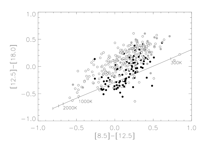
Figure 2: The [12.5]-[18.0] vs. [8.5]-[12.5] color-color diagram based on synthetic fluxes obtained from LRS data (see §2.2.1). Mira stars are shown as solid circles, NM (non-Mira) stars as open circles, and SRa stars as gray dots. The line is the locus of black-body colors parametrized by the temperature, as marked. Note the different distribution of Mira and NM stars.

Figure 3: Distribution of the [12.5]-[18.0] color excess, relative to a black body with the same [8.5]-[12.5] color temperature, for Mira (dashed line), NM (solid line) and SRa (dotted line) stars. Non-Mira stars have $\sim$0.2 mag larger color excess than Mira stars (see Table 1).

Sample	Median	Mean	$\sigma$	N
Mira	0.10	0.11	0.18	96
NM	0.34	0.32	0.18	246
SRa	0.37	0.33	0.19	48
spSR ($P<100$d)	0.37	0.36	0.17	57
lpSR ($P\ga 100$d)	0.32	0.30	0.20	130

Sample	F-test	t-test	result
Mira vs. NM	0.90	$6\cdot 10^{-20}$	Same $\sigma$, diff. mean
SRa vs. Mira	0.70	$2\cdot 10^{-10}$	Same $\sigma$, diff. mean
SRa vs. NM	0.60	0.71	Same $\sigma$ and mean
spSR vs. lpSR	0.16	0.05	Same $\sigma$ and mean

Table 1: Significance of statistical tests for the [12.5]-[18.0] color excess. Samples have different $\sigma$ at the 99% confidence level if the variance F-test returns a significance of 0.01 or smaller, and different mean values if Student’s t-test returns a significance of 0.01 or smaller

These two statistical tests suggest that, regarding their mid-IR [8.5]-[12.5] and [12.5]-[18.0] colors, Mira stars and NM stars are different. That is, given the envelope optical depth, as measured by the [8.5]-[12.5] color, NM stars show more cold emission measured by the [12.5]-[18.0] color. Among the SR sources, the mid-IR colors do not correlate with the pulsational period. Assuming the validity of the Kerschbaum & Hron (1992) correlation between the pulsational period and AGB evolution, this suggests that SR stars form similar circumstellar envelopes in the early and thermally pulsing AGB phases. The similarity of SRa with NM in general indicates that the SRa sample is not significantly contaminated by Mira stars.

2.2.2 The peak wavelength of the “9.7 $\mu$m” silicate feature

Following KHc, we also determine the peak wavelength of the “9.7 $\mu$m”silicate feature for all sources in the sample. Such studies were done first by Little-Marenin & Little (1990) who tried to classify LRS spectra for a large sample of AGB stars. They found that their subsample of SR and L variables showed a narrower silicate feature, and shifted to the red compared to Mira stars. A similar analysis was performed by Hron, Aringer & Kerschbaum (1997) for a larger number of sources, accounting for the dust continuum emission by fitting it with a separate black body. They confirmed the differences between the two classes, finding a shift of about 0.3 $\mu$m in the silicate feature peak position.

Figure 4: Distribution of the peak position of the silicate “9.7” $\mu$m feature for Mira (dashed line), NM (solid line) and SRa (dotted line) stars. The NM stars have the feature shifted for $\sim$0.2 $\mu$m with respect to the Miras.

We determine the silicate feature peak position by fitting a fifth degree polynomial to each LRS spectrum in the 9–11 $\mu$m wavelength range. This fitting procedure removes the effect of noise and eventual secondary features, producing “smooth” spectra where the position of the maximum can be easily recognized. The wavelength of the maximum of the fitting polynomial in the given interval is then assumed to be the position of the “true” silicate peak. With this technique we measured the position of the silicate peak for 85 Miras and 162 NM; for the remaining sources (11 Miras and 84 NM) the fitting procedure failed either because of the excessive noise in the spectra, or due to the absence of a significant feature. Many of the sources for which the silicate feature is too weak to measure the position of its peak are Lb stars of LRS class 1n.

The results for the position of the silicate feature peak are listed in Table 2 and shown as histograms in Figure 4. The mean values for Miras and NM are $\langle\lambda_{max}\rangle_{Mira}\simeq 9.86$ $\mu$m  and $\langle\lambda_{max}\rangle_{NM}\simeq 10.01$ $\mu$m  respectively; the medians are 9.87 and 10.08 $\mu$m. Note the different standard deviation $\sigma_{\lambda}$ of the two samples, almost twice as large for NM ($\sim 0.42$ $\mu$m) than for Miras ($\sim 0.28$ $\mu$m); this difference is 99.9% statistically significant according to the F-test. The Student’s t-test for the mean values, performed between the two samples (with unequal variances), confirms the separation of the Mira and NM populations with respect to their $\lambda_{max}$ at a high (99.95%) significance level, in agreement with the results of Hron, Aringer & Kerschbaum (1997).

Sample	Median	Mean	$\sigma$	N
Mira	9.87	9.86	0.28	85
NM	10.07	10.01	0.42	162
SRa	10.10	10.08	0.41	37
spSR ($P<100$d)	10.09	10.04	0.43	31
lpSR ($P\ga 100$d)	10.07	10.02	0.38	95

Sample	F-test	t-test	result
Mira vs. NM	$5\cdot 10^{-5}$	$5\cdot 10^{-4}$	Diff. $\sigma$ and meanb
SRa vs. Mira	$6\cdot 10^{-3}$	$4\cdot 10^{-3}$	Diff. $\sigma$ and meanb
SRa vs. NM	0.82	0.43	Same $\sigma$ and mean
spSR vs. lpSR	0.41	0.87	Same $\sigma$ and mean

Table 2: Significance of statistical tests for the peak Position of the silicate 9.7 $\mu$m feature. Samples have different $\sigma$ at the 99% confidence level if the variance F-test returns a significance of 0.01 or smaller, and different mean values if Student’s t-test returns a significance of 0.01 or smaller

We performed the same test on the SRa class alone, finding $\langle\lambda_{max}\rangle_{SRa}\simeq 10.08$ $\mu$m, and $\sigma_{\lambda}\simeq 0.41$, consistent with the results for the whole NM class. This further indicates that the SRa subsample does not contain a significant number of misclassified Miras. The $\langle\lambda_{max}\rangle$ values for the NM subsets with $P\ga 100$ ^d  and $P<100$ ^d  are 10.07 and 10.09 $\mu$m  respectively, and the $\sigma_{\lambda}$ are 0.43 and 0.39 $\mu$m. The difference in the $\sigma_{\lambda}$ of the two subsample is not significant, confirming that the two subsets are part of the same population, in agreement with the analysis of synthetic mid-IR colors.

2.3 Interpretation of the Observed Differences

We have shown that oxygen rich Mira and non-Mira stars have statistically different properties of their infrared emission. In particular, we find

1. Different distribution in the K-[12] vs. [12]-[25] color-color diagram.

2. Different [12.5]-[18.0] excess emission

3. Different peak position of the silicate feature

As shown by IK98 (c.f. Figure 1), these differences are not in agreement with the “standard” steady-state radiatively driven wind models: while they can reproduce the properties of the Mira sample, they cannot explain the infrared emission from non-Mira stars. There are three ways to augment the “standard” models without abandoning the hypothesis of a radiatively driven outflow: changing the input (stellar) spectrum, altering the spectral shape of dust opacity, and employing a different dust density distribution.

The star in the “standard” models is assumed to radiate as a 2500 K black-body. The observed differences in the K-[12] vs. [12]-[25] color-color diagram could imply that typical stellar temperature is significantly different for Mira vs. non-Mira stars, or that black-body spectral shape is not an adequate description of the true stellar spectrum (e.g. due to an absorption feature in K band like H₂O feature seen in IRTS data by Matsuura et al. 1998). A different input spectrum would affect the model K flux, and to some extent the 12 $\mu{\rm m}$ flux in optically thin envelopes. However, such a change cannot account for the observed differences in the mid-infrared region (items 2 and 3 above) where the flux is dominated by dust emission.

It is possible to produce model spectra in agreement with data for non-Miras by altering the adopted spectral shape of absorption efficiency for silicate grains. There are two required changes. First, the ratio of silicate feature strengths at 18 $\mu{\rm m}$ and 10 $\mu{\rm m}$ has to be increased for a factor of about 2-3 . Such a change results in a model track in the K-[12] vs. [12]-[25] diagram which leaves the Rayleigh-Jeans point at a larger angle (with respect to K-[12] axis) than before, and passes through the observed source distribution. These models also produce larger [12.5]-[18.0] excess emission in agreement with item 2 above. In order to account for item 3 above, a second change is required: the peak position of the “9.7” micron feature has to be shifted longwards for about 0.2-0.3 $\mu{\rm m}$. For example, the inclusion of Al oxides can shift the peak position to longer wavelengths (Speck et al. 2000). We conclude that, although the postulated changes might seem ad hoc and have little support from model dust optical properties, the possibility of non-Miras having somewhat different grains cannot be ruled out by using near-IR and IRAS data alone.

The third way to alter the model spectra predicted by “standard” models is to decrease T₁, the dust temperature at the inner envelope edge, which is usually assumed to correspond to the dust condensation temperature ($\sim$1000 K). The removal of hot dust reduces the flux at 12 $\mu{\rm m}$ significantly more than the fluxes in K band and at 25 $\mu{\rm m}$, and produces model tracks in agreement with the source distribution in the K-[12] vs. [12]-[25] color-color diagrams (c.f. Figure 1), and larger [12.5]-[18.0] excess emission. It is remarkable that the models with a low $T_{1}$ are also capable of explaining the differences between the peak position of the silicate feature. The top panel in Figure 5 displays two model spectra obtained with visual optical depth of 0.6, and T₁ = 300 K (dashed line) and 700 K (solid line). The dotted line shows the stellar spectrum. Because the hot dust has been removed in the model with T₁ = 300 K, both the blue and red edges of the 10 $\mu{\rm m}$ silicate emission feature are shifted longwards for about 0.2-0.3 $\mu{\rm m}$. While the peak position in the model spectra is exactly the same in both models, the addition of noise to the models would make the whole feature for T₁ = 300 K model appear shifted longwards. Thus, assuming a lower T₁ in models for NM stars can account for all 3 items listed above. Such models are further described in the next section.

Figure 5: Model spectra in the LRS region obtained for silicate grains with the visual optical depth of 0.6 and 2 values of the dust temperatures at the inner envelope radius, T₁ (solid and dashed lines). Dotted line shows the stellar contribution to the spectra. Note that the silicate “9.7” $\mu$m feature appears weaker and is shifted longwards for T₁ = 300 K, relative to the position obtained for T₁ = 700 K, although both are calculated with the same grain optical properties.

We conclude that the two most probable explanations for the observed differences in infrared emission between Mira and non-Mira stars are either different grain optical properties, or the lack of hot dust in non-Mira stars. The possibility that employing different types of grains could reproduce the observed differences between Mira and NM stars requires extensive modeling effort and will be analyzed in a separate publication (Helvaçi et al. 2001). Here we discuss low-T₁ models and show that they are consistent with the infrared emission observed for NM stars. Various observational techniques for distinguishing these two hypothesis are further discussed in §4.

3 MODELS

3.1 Model Assumptions and Predictions

We calculate model spectra by using the DUSTY code (Ivezić, Nenkova & Elitzur, 1997). It is assumed that the star radiates as a 2500 K black-body. Silicate warm dust opacity is taken from Ossenkopf et al. (1992), with the standard MRN grain size distribution (Mathis, Rumpl & Nordsiek, 1977). Dust density is described by $r^{-2}$ with an arbitrary inner envelope radius, $r_{1}$. The outer envelope radius is irrelevant as long as it is much larger than $r_{1}$, and we fix it at the value of $3\times 10^{17}$ cm. In the interrupted mass loss model, the inner envelope radius increases with $t$, the time elapsed since the mass loss stopped as

$$r_{1}=r_{1}(0)+{\rm v}\,t=r_{1}(0)+3.2\times 10^{13}\,{\rm cm}\,\,v_{10}\,\hbox{${\rm t_{yr}}$}$$ (1)

where $t$ = ${\rm t_{yr}}$ years, the expansion velocity v = $v_{10}$ 10 km s^-1, and $r_{1}(0)$ is the envelope inner radius at $t=0$. This radius depends on the grain optical properties and dust condensation temperature, and the stellar temperature and luminosity (IE97). For typical values

$$r_{1}(0)=3\times 10^{14}\,{\rm cm}\,\,L_{4}^{1/2},$$ (2)

where the stellar luminosity $L=L_{4}10^{4}$ $L_{\odot}$.

We specify $r_{1}$ by the temperature at the inner edge at time $t$, T₁. This temperature decreases with time because the distance between the star and the envelope inner edge increases. This relationship is approximately given by (IE97, eq. 30)

$${T_{1}\over T_{1}(0)}=\left({r_{1}(0)\over r_{1}}\right)^{2\over 4+\beta}$$ (3)

where $\beta$ is the power-law index describing the opacity wavelength dependence. This expression is strictly correct only in the optically thin regime, and furthermore, the silicate dust opacity cannot be described by a simple power law. However, it provides a good description of detailed model results with $\alpha=2/(4+\beta)\hbox{$\sim$}0.40\pm 0.05$. Combining the above expressions gives

$${T_{1}\over T_{1}(0)}=\left(1+0.1{v_{10}\hbox{${\rm t_{yr}}$}\over L_{4}^{1/2}}\right)^{-\alpha}.$$ (4)

As already indicated in §2 (c.f. Figure 1), the distribution of SR stars in the K-[12] vs. [12]-[25] color-color diagram implies a lower limit on $T_{1}$ of $\sim$300 K. Assuming $T_{1}(0)$ = 800 K, $v_{10}=L_{4}=1$ implies a time scale of 100 yr.

The second free parameter is the dust optical depth which we specify as the visual optical depth, $\tau_{V}$. This parameter controls the amount of dust and increases with $\dot{\rm M}$, the mass-loss rate during the high mass loss phase. The steady-state radiatively driven wind models give for silicate dust (Elitzur & Ivezić 2000)

$$\hbox{$\dot{\rm M}$}=2\times 10^{-6}\,\hbox{$M_{\odot}$}\,{\rm yr}^{-1}\,\hbox{$\tau_{V}$}(0)^{3/4}\,L_{4}^{3/4}\left(r_{gd}\over 200\right)^{1/2}$$ (5)

where $r_{gd}$ is the gas-to-dust ratio, and $\tau_{V}$(0) is the optical depth before the mass loss stops. Note that $\dot{\rm M}$ $\propto\hbox{$\tau_{V}$}^{3/4}$ rather than $\dot{\rm M}$ $\propto$ $\tau_{V}$ due to dust drift effects.

After the mass loss stops, the optical depth decreases with time because it is inversely proportional to $r_{1}$ due to the envelope dilution

$${\hbox{$\tau_{V}$}\over\hbox{$\tau_{V}$}(0)}=\left(1+0.1{v_{10}\hbox{${\rm t_{yr}}$}\over L_{4}^{1/2}}\right)^{-1}.$$ (6)

The models could be parametrized by $\dot{\rm M}$ and $r_{1}$ (or $t$) instead of $\tau_{V}$ and $T_{1}$. However, in such a case the parametrization of a model spectrum would involve at least two additional parameters ($L$ and $r_{gd}$) and would artifically introduce a four-dimensional fitting problem. As the scaling properties of the radiative transfer imply (IE97), the described model is only a two-dimensional problem fully specified by $\tau_{V}$ and $T_{1}$. It is only the correspondence between these two parameters and other quantities such as $\dot{\rm M}$ that involves additional assumptions about e.g. $r_{gd}$.

In the interrupted mass loss model the changes of $T_{1}$ and $\tau_{V}$ as the envelope expands are correlated. Combining eqs. (4) and (6) gives

$${T_{1}\over T_{1}(0)}=\left({\hbox{$\tau_{V}$}\over\hbox{$\tau_{V}$}(0)}\right)^{\alpha},$$ (7)

and thus during the expansion

$$T_{1}\hbox{$\tau_{V}$}^{-\alpha}=C=const.$$ (8)

where the value of constant C is determined by $\dot{\rm M}$ during the high mass loss phase. The model predicts that the distribution of best-fit $T_{1}$ and $\tau_{V}$ should resemble a strip in the $\tau_{V}$–$T_{1}$ plane whose width is determined by the intrinsic distribution of the mass-loss rates during the high mass-loss rate phase, and with the position along the strip parametrized by the time since the mass loss stopped.

Another model prediction is for the $T_{1}$ distribution of sources in an unbiased sample (or equivalently for the $\tau_{V}$ distribution since $\tau_{V}$ and $T_{1}$ are correlated). Eq. (4) shows that the first derivative of $T_{1}$ decreases with time and thus the number of observed sources should increase as $T_{1}$ decreases. Assuming $dN(T_{1})\propto dt(T_{1})$, where $dN$ is the number of sources in a given $T_{1}$ bin, the model implies

$${dN\over dT_{1}}\propto T_{1}^{-{1+\alpha\over\alpha}}\propto T_{1}^{-3.5}.$$ (9)

This prediction applies for sources with $T_{1}$ smaller than the dust condensation temperature, $T_{c}$. The number of sources with $T_{1}$ comparable to $T_{c}$ depends on the duration of the high mass loss phase such that the ratio of the number of sources with $T_{1}<T_{c}$, to the number of sources with $T_{1}\hbox{$\sim$}T_{c}$, is equal to the ratio of times spent in the low and high mass-loss phases.

Figure 6: An illustration of the two-dimensionality of LRS spectra. Each column displays a time evolution of model spectra after the mass loss interruption, calculated in steps of 25 years. The spectra in 3 columns are displayed for different mass-loss rates before the interruption, increasing from left to right, and indicated on top of each column. Each spectrum is fully characterized by $\tau_{V}$ and $T_{1}$, which equivalently can be expressed as time $t$, marked in each panel, and mass-loss rate. The corresponding values of LRS class, which measures the 9.7 $\mu$m silicate feature strength, and the F₁₈/F₁₀ ratio are also marked in each panel (see text for details).

To summarize, the interrupted mass loss models assume a sudden drop in the mass-loss rate after which the envelope freely expands. The infrared spectrum emitted during this phase depends on only two free parameters, the temperature at the inner envelope edge, $T_{1}$ and the envelope optical depth $\tau_{V}$. Both of these quantities decrease with time in a correlated way described by eq. (8).

Note that the two free parameters imply a two-dimensional family of model LRS spectra. It is usually assumed that the shape of an LRS spectrum for silicate grains is fully specified by the 9.7 $\mu$m silicate feature strength. However, in this model even for a fixed 9.7 $\mu$m silicate feature strength, there is a family of spectra with differing shapes due to the varying second parameter. We find that the ratio of fluxes at 18 $\mu$m and 10 $\mu$m, F₁₈/F₁₀, is a convenient observable, in addition to the 9.7 $\mu$m silicate feature strength, which can be used to parametrize the LRS spectra. That is, each combination of $T_{1}$ and $\tau_{V}$ corresponds to a unique combination of the 9.7 $\mu$m silicate feature strength and the F₁₈/F₁₀ ratio, and each such LRS spectrum corresponds to a unique pair of $T_{1}$ and $\tau_{V}$. Of course, assuming that all stars have the same $L$, $r_{gd}$ and $v_{10}$, a given LRS spectrum corresponds to a unique combination of $\dot{\rm M}$ and $r_{1}$, and vice versa.

This two-dimensionality of LRS spectra is illustrated in Figure 6 which displays a time evolution of model spectra after the mass loss interruption (for details see the figure caption). Each spectrum is fully characterized by $\tau_{V}$ and $T_{1}$, which equivalently can be expressed as time $t$, marked in each panel, and mass-loss rate indicated on top of each column. The corresponding values of LRS class, which measures the 9.7 $\mu$m silicate feature strength, and the F₁₈/F₁₀ ratio are also marked in each panel. Note that some spectra have the same LRS class (e.g. $t$=0 yr in the first column, $t$=25 yr in the second column, and $t$=50-75 yr in the third column) and yet are clearly distinguishable both by their overall shape and the values of the F₁₈/F₁₀ ratio. Another important detail is that the spectra with comparatively large F₁₈/F₁₀ ratio are obtained only for comparatively low $T_{1}$, as discussed earlier.

While we assume that the mass loss ceases completely, the data provide only a lower limit on the mass-loss rate ratio in the two phases of high and low mass loss. We have explored a limited set of models where the mass-loss rate drops for a factor 3, 5, 10, and 100, and found that with the available data we cannot distinguish cases when the mass-loss rate drops by more than a factor of 5. Thus, this is a lower limit on the ratio of mass-loss rates in the two phases.

We have computed $\sim$2000 model spectra parametrized on logarithmic grids with 62 $\tau_{V}$ steps in the range $10^{-3}$–350, and 32 $T_{1}$ steps in the range 100 K – 1400 K. Models calculated on a finer grid in either $\tau_{V}$ or $T_{1}$ vary less between two adjacent grid points than typical noise in the data. A subset of models with $T_{1}$ restricted to the interval 600–1400 K is hereafter called “hot-dust” models. We separately fit these models to all sources in order to test whether “cold-dust” models (with $T_{1}<$ 600 K) are necessary to improve the fits.

3.2 Fitting Technique

The best fit model for each source is found by using a $\chi^{2}$ minimization routine applied to the source and model spectra in the IRAS LRS spectral region (8 $\mu$m– 23 $\mu$m). The $\chi^{2}$ variable is defined as

$$\chi^{2}=\frac{1}{N-2}\sum_{i=1}^{N}\frac{\left[\lambda_{i}F^{O}_{\lambda}(\lambda_{i})-\lambda_{i}F^{M}_{\lambda}(\lambda_{i})\right]^{2}}{\sigma_{O}^{2}+\sigma_{M}^{2}},$$ (10)

where $F^{O}_{\lambda}$ is the observed flux and $F^{M}_{\lambda}$ is the model flux. The error $\sigma_{O}$ of the IRAS LRS data was estimated as the root-mean-square (rms) difference between the raw and a cubic spline smoothed LRS spectra. The model error $\sigma_{M}$ is taken as the rms difference between the two closest models in the parameter space. The $\chi^{2}$ variable was then normalized to the number of wavelengths $N$, minus the number of fitting parameters ($\tau_{V}$ and $T_{1}$). By comparing each source spectrum with all spectra in a given model set, we determine the $\chi^{2}$ and select a model with the lowest $\chi^{2}$ as the best-fit model. This procedure is repeated independently for the set of all models, and for the “hot dust” subset.

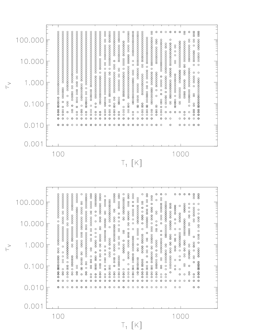
Figure 7: Test diagram of the fitting procedure. Gaussian noise with SNR = 10 (top) and 5 (bottom) is added to the full grid of models and the resulting spectra are fitted with the noiseless spectra. Each circle represent a successful recovery of the true $\tau_{V}$ and $T_{1}$, while the missing points are incorrectly identified models. The majority of “failed” models fall on to a neighboring grid point.

As discussed in the previous section, the interrupted mass loss model predicts a particular distribution of sources in the $\tau_{V}$–$T_{1}$ plane, which may be affected by hidden systematic biases in the fitting procedure. In order to assess the level of such biasing, we perform a “self-fit” test for all models in the sample. We add Gaussian noise similar to the noise in the LRS data to each of the DUSTY model spectra and then pass such spectra through the fitting algorithm. We consider two noise levels (signal-to-noise ratio, SNR), SNR = 10 typical for the whole sample and SNR = 5 representative of the stars with the lowest-quality LRS data.

The results are shown in Figure 7 where each circle represents a point in the model grid; missing points are models for which the true $\tau_{V}$ and $T_{1}$ were not recovered due to noise in the “data”. The majority of such “failed” fits fall on to a neighboring grid point. The figure shows that increasing noise can reduce the effectiveness of our procedure. However, the $T_{1}$ distribution of the incorrectly identified models is uniform even in the low SNR case, and thus within the limits of our sample the fitting procedure does not introduce significant biasing in the best-fit parameters.

3.3 Best-fit Model Results

The quality of a fit is described by the best fit $\chi^{2}$ variable. A good fit, in which the details of the source spectra are reproduced by the model (e.g. Figure 8, panel $a$), generally has $\chi^{2}\la 5$. Fits with $5\la\chi^{2}\la 10$ are still acceptable, even though some secondary features in the source spectrum cannot be fully reproduced by the model. This seems to be mainly due to the inability of the adopted silicate opacity to describe all observed spectral features (e.g. the 13 $\mu$m feature). A larger $\chi^{2}$ ($\ga$10) indicates more serious discrepancies in the fit, that can range from the convergence errors (e.g. when the fitting routine cannot find a well defined minimum in the $\chi^{2}$ surface) to poor fits indicating that the adopted opacity and/or radial dust density law are grossly inadequate. Such sources represent less than 10% of the sample.

3.3.1 The Fit Quality

The statistics of the best-fit $\chi^{2}$ values for sources with $\chi^{2}<10$ are shown in Table 3. The table reports the fraction of sources in each subsample (Mira, NM, SRa, spSR, and lpSR) which cannot be fitted with a $\chi^{2}$ less than 3 and 10 (“excellent” and “acceptable” fits). The sources are fitted with two sets of models: “all temperatures” models which include the full $T_{1}$ grid, and the “hot dust” models with $T_{1}>600$ K. As evident, a larger fraction of sources in all subsamples can be fitted within a specified $\chi^{2}$ limit with the “all” model set than with the “hot dust” models. This is not surprising since the former model set includes a greater variety of spectra due to the two free parameters, as opposed to the restrictions on one free parameter in the latter set. Nevertheless, the improvement in the best fit quality is more significant for the NM sample (and all NM subsamples) than for Mira stars. For example, more than a half of NM stars cannot be fitted with a $\chi^{2}<3$ by using “hot dust” models, while the inclusion of models with low $T_{1}$ decreases their fraction to less than 20%. At the same time, the corresponding fractions for Mira stars are 42% and 35% indicating that low-$T_{1}$ models are not necessary to model LRS data of these stars.

Sample	$\chi^{2}$$\la$$3$	$\chi^{2}$$\hbox{$\la$}10$		$\chi^{2}$$\la$$3$	$\chi^{2}$$\hbox{$\la$}10$
	all	models		hot	dust
Mira	35%	3%		42%	12%
NM	18%	1%		54%	22%
SRa	21%	2%		33%	4%
spSR ($P<100$d)	18%	0%		67%	21%
lpSR ($P\ga 100$d)	21%	2%		48%	6%

Table 3: The best fit statistics. The table lists the fraction of sources in each subsample which cannot be fitted with the specified $\chi^{2}$ criteria. The second and third column correspond to “all” (temperature) models, and the third and fourth column to “hot dust” models (see text).

An example of the improvement in the fit quality due to a lower $T_{1}$ is shown in Figure 8. The model spectra are plotted by dashed dotted lines and the IRAS LRS data by solid lines. In panel $a$ the SRb star TY Dra is fitted with a cold dust model ($T_{1}\simeq 370$ K), resulting in a very small $\chi^{2}$. When the dust temperature is limited to the range 600–1400 K, the fit is unable to reproduce the source spectral energy distribution, as shown in panel $b$. The panels $c$ and $d$ show good quality fits of a Mira star with relatively hot dust ($T_{1}$ = 825 K) and an SR star with very low inner shell temperature ($T_{1}$ = 270 K).

Figure 8: An example of model fits (dashed dotted line) to the IRAS LRS data (solid line) for Mira and NM sources. In panel $a$ the SRb star TY Dra is fitted with a cold dust model ($T_{1}\simeq 370$ K), resulting in a very small $\chi^{2}$. When the dust temperature is limited to the range 640–1400 K, the fit is unable to reproduce the source spectral energy distribution, as shown in panel $b$. The panels $c$ and $d$ show good quality fits of a Mira star with relatively hot dust ($T_{1}=825$ K) and an SR star with very low inner shell temperature ($T_{1}=270$ K).

3.3.2 Distribution of Best-fit Parameters

The distribution of best-fit $\tau_{V}$ and $T_{1}$ is shown in Figure 9. Sources from Mira and NM subsamples are marked by solid and open circles, respectively (since the differences in best-fit parameters between the various subsamples of NM stars are not statistically significant, we consider only Mira/NM subsamples hereafter). A small random offset (up to 1/3 of the parameter grid step) has been added to each $T_{1}$ and $\tau_{V}$, in order to separate the sources with identical best fit parameters, which would otherwise appear as a single point on the diagram. The sources are distributed not randomly but rather along a diagonal strip. The density of sources along the strip has a local minimum for $T_{1}$ $\sim$500 K ($\tau_{V}$$\sim$5) suggesting a division into four regions as shown by the thin solid lines. The source counts in the quadrants, labeled clockwise from I to IV, are given in Table 4. Although both Mira and NM stars are present along the whole strip, Mira tend to aggregate in the upper right quadrant with higher $T_{1}$ and $\tau_{V}$. On the contrary, NM stars aggregate in the lower left quadrant with $T_{1}<$ 500 K and $\tau_{V}<$ 0.5.

Sample	I	II	III	IV
Mira	59	1	32	1
NM	72	2	169	1
SRa	20	1	26	0

Table 4: The source distribution in $\tau_{V}$ vs. $T_{1}$ diagram (see Figure 9).

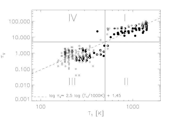
Figure 9: The distribution of best-fit $\tau_{V}$ and $T_{1}$ for Mira stars (solid circles) and non-Mira stars (open circles). A small random offset (up to 1/3 of the parameter grid step) has been added to each $T_{1}$ and $\tau_{V}$, in order to separate the sources with identical best fit parameters, which would otherwise appear as a single point on the diagram. The plot is divided in four regions, according to the source segregation; the counts in the four quadrants are given in Table 4.

The strong correlation between the best-fit $\tau_{V}$ and $T_{1}$ seen in Figure 9 is probably not due to hidden biasing of the fitting algorithm (c.f §3.2). Indeed, such correlation is expected in the interrupted mass loss model as discussed in §3.1. Eq.(8) predicts $\tau_{V}$$\propto$ $T_{1}^{1/\alpha}$ = $T_{1}^{2.5}$ shown as a thick dashed line in Figure 9. The close agreement between the source distribution and predicted correlation is evident. Fitting a power law to the source distribution gives a best-fit power-law index of 2.8 for Mira stars, and 2.5 for NM stars, consistent with the model prediction, given the uncertainty of $\alpha$ ($\pm 0.05$).

Another model prediction pertains to the distribution of best-fit $T_{1}$. For sources in the quiescent phase, eq. (9) predicts $dN/dT_{1}$ $\propto$ $T_{1}^{-3.5}$, or equivalently, $dN/dlog(T_{1})$ $\propto$ $T_{1}^{-2.5}$. The histogram of best-fit $T_{1}$ is shown in Figure 10 for Mira stars (dashed line) and NM stars (solid line). The relation $dN/d\log(T_{1})$ $\propto$ $T_{1}^{-2.5}$ is shown as a dotted line, normalized to the NM bin with $T_{1}$ $\approx$ 200 K. It is evident that the $T_{1}$ distribution is very different for Mira and NM stars. While this distribution is flat for Mira stars, with about 2/3 of stars having $T_{1}>$ 500 K, 2/3 of NM stars have $T_{1}<$ 500 K. These stars closely follow the model prediction for stars whose envelopes are freely expanding after their mass loss has stopped.

The low-$T_{1}$ of the NM distribution in Figure 10 abruptly ends at $T_{1}$ $\sim$200 K although the model grid extends to $T_{1}$ = 100 K. As discussed in IK98, this sharp end may indicate that the mass loss resumes after the quiescent phase because otherwise the envelopes with 100 K $<T_{1}<$ 200 K should be detected. Eq. (4) implies that the time scale for the envelope expansion until $T_{1}$ reaches such a low temperature is of the order 100 years. If the mass loss starts again, in less than 10 years the new shell would occupy the region where the dust temperature is higher than about 600 K, and thus about 10% of stars could be in this phase. The only difference between such a double-shell envelope and a steady-state envelope with smooth $r^{-2}$ dust density distribution is the lack of dust with temperatures in the range 200–600 K. Detailed model spectra in the spectral range 5-35 $\mu$m for such double-shell envelopes show that they are practically indistinguishable from spectra obtained for envelopes with $r^{-2}$ dust density distribution.

The fraction of NM stars with $T_{1}>$ 500 K is $\sim$1/3. This fraction provides an upper limit for the duration of high mass loss phase of $\sim$50 years. However, it would not be surprising if this estimate is wrong by perhaps a factor of 2 since the analysis presented here only provides a lower limit on the ratio of mass-loss rates in the high and low mass loss phases. Thus, the observations do not strongly exclude the possibility that the duration of both phases may be the same.

Figure 10: Histogram of best-fit $T_{1}$ for Mira stars (dashed line) and NM stars (solid line). The dashed line shows relation dN/dlog($T_{1}$) $\propto$ $T_{1}^{-2.5}$, normalized to the NM bin with $T_{1}\approx$ 200 K.

3.4 The Distribution of Mass-loss Rates

The width of the strip formed by the source distribution in the $\tau_{V}$ vs. $T_{1}$ diagram (Figure 9) is determined by the intrinsic distribution of mass-loss rates. We calculate mass-loss rates from the best-fit $\tau_{V}$ and $T_{1}$ by using

$$\hbox{$\dot{\rm M}$}=\hbox{$\tau_{V}$}^{3/4}\left(1000\,{\rm K}\over T_{1}\right)^{2.5}10^{-6}\,\hbox{$M_{\odot}$}\,{\rm yr}^{-1}$$ (11)

which is derived by combining eqs. (5-7) and assuming $(T_{1}(0)/1000{\rm K})^{2.5}\,L_{4}^{3/4}\,(r_{gd}/200)^{1/2}=0.5$. Figure 11 shows the histograms of calculated mass-loss rates for Mira stars (dashed line) and NM stars (solid line). The histograms are rather narrow, and furthermore, they are the same within the uncertainties, according to F-test and t-test analysis. Such a similarity of mass-loss rates between Mira and NM stars is somewhat surprising because a “standard” result is that NM stars have several times smaller mass-loss rates than Mira stars (e.g. Habing 1996). A plausible explanation for the smaller mass-loss rates usually derived for NM stars may be the lack of correction for lower $T_{1}$ (c.f. eq. 11) when converting the envelope optical depth to mass-loss rate. The results presented here indicate that the majority of both Mira and NM stars have mass-loss rates of the order 10^-5. An alternative explanation is that the KHc sample of NM stars is biased towards high mass-loss rates, although such an effect is not expected for their selection procedure. Additional selection criteria employed in this work did not affect a sufficiently large number of NM sources to result in such biasing. It is not possible to distinguish between those two possibilites without a large and unbiased sample with uniformly measured mass-loss rates by an IR-independent method (e.g. molecular emission).

Figure 11: Histogram of derived mass-loss rates for Mira stars (dashed line) and NM stars (solid line).

4 DISCUSSION

The analysis presented here shows that the observed differences in infrared emission from oxygen rich AGB stars of different variability type are statistically significant. Mira stars and NM stars clearly segregate in the K-[12] vs. [12]-[25] color-color diagram, and also have different detailed properties of their IRAS LRS spectra. We find no statistically significant differences between various subsamples of NM stars. The differences between Mira and NM stars are hard to interpret in the context of steady state wind models. In particular, these models do not provide satisfactory description of the infrared emission from the majority of NM stars. Possible ways to augment these models include changing the shape of stellar spectrum, employing grains with altered absorption efficiency, or assuming that the majority of NM stars have envelopes without hot dust ($\ga$ 500 K).

We find that the absence of hot dust for NMs is the most plausible way to explain the observations, although the available data cannot rule out the possibility that the differences in circumstellar dust chemistry produce the observed differences in infrared emission. For example, Sloan et al. (1996) found that the “13 micron” feature occurs somewhat more frequently in SRb stars (75%-90%) than in all AGB stars with silicate dust (40%-50%). On the other hand, this difference could be simply due to different densities in the dust formation region, as pointed out by Speck et al. (2000). We are in the midst of a detailed study exploring the model spectra obtained for a large sample of different dust types and grain size distributions (Helvaçi et al. 2001).

We provide detailed analysis of models where the absence of hot dust for NM stars is interpreted as an interruption of the mass loss with time scales of the order 100 years, and a drop in the mass-loss rate of at least a factor of 5. In such a case, envelope freely expands and the dust temperature decreases with time. This hypothesis predicts a correlation $\tau_{V}$$\propto T_{1}^{2.5}$ between the envelope optical depth, $\tau_{V}$ and the dust temperature at the inner envelope edge, $T_{1}$, which we find consistent with the data. We find that the model prediction for the distribution of best-fit $T_{1}$ also agrees with the data, although this constraint may be plagued by hidden biases in the sample. We interpret the sharp low-$T_{1}$ end of the source distribution as evidence that the mass loss resumes and estimate the duration of high mass loss phase to be of the same order as the duration of the low mass loss phase.

The number of Mira stars with low $T_{1}$ is about 1/3 and it is not clear from the present analysis whether this represents evidence for the interrupted mass loss. It was proposed by Kerschbaum et al. (1996), based on similar number densities and scale heights, that AGB stars oscillate between NM and Mira phases. This idea was further advanced by IK98 based on their analysis of the source distribution in the K-[12] vs. [12]-[25] diagram. However, recent results by Lebtzer & Hron (1999), who compare the abundance of ⁹⁹Tc in a large sample of SR stars and Mira stars, seem to rule out this hypothesis. The ⁹⁹Tc abundance is characterized by a quick increase during the first thermal pulse, after which it presumably stays constant (Busso et al. 1992). Consequently, a similar fraction of Tc-rich stars should be found in the Mira and SR samples, contrary to the observations by Lebtzer & Hron who find that a fraction of stars with detectable Tc is lower for SR stars (15%) than for Mira stars (75 %).

While the available observations are consistent with the interrupted mass loss model, the possibility that observed differences between Mira and NM stars are due to different dust optical properties can not be excluded by considering photometric data alone. The most obvious and direct test of the interrupted mass loss hypothesis is mid-IR imaging. When T₁ decreases by a factor of two, the inner envelope radius increases by about a factor of four. Such a difference should be easily discernible for a few dozen candidate stars with largest angular sizes, which are already within the reach of the Keck telescopes (e.g. Monnier et al. 1998). Molecular line observations can also be used to infer the gas radial density distribution because various lines form at different radii. For example, SiO8-7 (347.3 GHz) line is expected to form much closer to the star than, say, CO3-2 (345.8 GHz) line. If SRb/Lb stars really lack material in the inner envelope, they should have lower SiO8-7/CO3-2 intensity ratios than Miras, provided that the excitation mechanisms are similar. Another, indirect, test can be made by employing mass-loss rates determined in molecular, either thermal or maser observations. For a given mass-loss rate, NM stars should have bluer 12-K color because their dust optical depth becomes smaller as the envelope expands. While this effect is not very pronounced (difference is about 0.2-0.3 magnitudes), a sufficiently large sample might provide statistically meaningful results.

For a few stars there are available spatially resolved observations (c.f. §1) and they seem to indicate mass loss changes with short time scales ($<$ several hundred years). If proven correct, the mass-loss variations on time scale of about 100 years would significantly change our understanding of the stellar evolution on the AGB since the known time scales are either much shorter (stellar pulsations, $\sim$1 year), or much longer (He flashes, $\sim$10⁵ years). However, the time dependent wind models (Winters 1998) seem to produce mass-loss rate variations with time scales much longer that the pulsation period which drives the mass loss ($\sim$1 year). These longer time scales are not fully understood (see however Deguchi 1997) and seem to result from the complex interplay between the pulsation and dust formation and destruction mechanisms. While the theoretically obtained time scales (5–10 years) are shorter than those implied by the observations, the recent developments show that it may be possible to increase the model time scale to $\sim$100 yr (Winters J.M., priv. comm.). It is not clear why would Mira and non-Mira stars exhibit different behaviors, unless the coupling mechanisms are very sensitive to the details of the pulsation mechanism (see e.g. Mattei et al. 1997).

Another possibility is that the 100-year mass-loss rate modulations are caused by the luminosity variations on similar time scales (Sahai et al. 1998). Recent work based on the analysis of stars observed by both the IRAS and HIPPARCOS surveys (Knauer, Ivezić & Knapp 2000) shows that the extensive mass loss on the AGB seems to require a threshold luminosity of $\sim$2000 $L_{\odot}$. If the luminosity of non-Mira stars oscillates around this value, then the resulting mass-loss rate would be in agreement with the model assumptions discussed here. Within this hypothesis Mira stars could have slightly larger luminosities (for perhaps a factor of 2) and exhibit a steady mass loss, a possibility that seems to be consistent with the P-L relation since Mira stars have somewhat longer periods that SR stars (Whitelock 1986).

References

- [1]
- [2] Bedding, T.R., Zijlstra, A.A., Jones, A., & Foster, G. 1998, MNRAS, 301, 1073
- [3] Bedijn, P.J. 1987, A&A, 186, 136
- [4] Busso, M., Gallino, R., Lambert, D.L., Raiteri, C.M., & Smith, V.V. 1992 ApJ, 399, 218
- [5] Busso, M., Origlia, L., Marengo, M., Persi, P., Ferrari-Toniolo, M., Silvestro, G., Corcione, L., Tapia, M., Bohigas, J. 1996, A&A, 311, 253
- [6] Deguchi, S. 1997, in IAU Symp. 180, Planetary Nebulae, ed. H. Lamers & H.J. Habing
- [7] Draine, B.T., & Lee H.M. 1984, ApJ, 285, 89
- [8] Elitzur M., & Ivezić, Ž. 2000, submitted to MNRAS
- [9] Gilman, R.C. 1969, ApJ, 155, L185
- [10] Habing, H. 1996, A&A Rev., 7, 97
- [11] Habing, H.J., Tignon, J., & Tielens, A. G. G. M. 1994, A&A, 286, 523
- [12] Harpaz, A., Rappaport, S., & Soker, N. 1997, ApJ, 487, 809
- [13] Hashimoto, O., Izumiura, H., Kester, D.J.M., & Bontekoe, Tj. R. 1998, A&A, 329, 213
- [14] Helvaçi, M. et al. 2001, in prep.
- [15] Hron, J., Aringer, B., & Kerschbaum F. 1997, A&A, 322, 280
- [16] Ivezić, Ž., & Elitzur M. 1995, ApJ, 445, 415 (IE95)
- [17] Ivezić, Ž., & Elitzur M. 1996, MNRAS, 279, 1011
- [18] Ivezić, Ž., & Elitzur M. 1997, MNRAS, 287, 799 (IE97)
- [19] Ivezić, Ž., Nenkova M., & Elitzur M. 1997, User Manual for DUSTY, Internal Report, University of Kentucky, accessible at http://www.pa.uky.edu/~moshe/dusty
- [20] Ivezić, Ž., Knapp, G.R., & Elitzur M. 1998, Proceedings of the 6th Annual Conference of the CFD Society of Canada, June 1998, Québec, p. IV-13; also astro-ph/9805003
- [21] Ivezić, Ž., & Knapp, G.R. 1998, Proceedings of the I.A.U. Symposium 191 “AGB Stars”, August 27 - September 1, 1998, Montpelier, France, p. 395; also astro-ph/9812421 (IK98)
- [22] Jura, M., & Kleinmann, S.G. 1992, ApJS, 83, 329
- [23] Justtanont, K., Feuchtgruber, H., de Jong, T., Cami, J., Waters, L.B.F.M., Yamamura, I., & Onaka, T. 1998, A&A, 330, L17
- [24] Kerschbaum, F., & Hron, J. 1992, A&A, 263, 97
- [25] Kerschbaum, F., & Hron, J. 1994, A&AS, 106, 397
- [26] Kerschbaum, F., & Hron, J. 1996, A&A, 308, 489
- [27] Kerschbaum, F., Olofsson, H., & Hron, J. 1996, A&A, 311, 273
- [28] Kholopov, P.N., Samus, N.N, Frolov, M.S., et al. 1985-1988, General Catalogue of Variable Stars, 4th edition, “Nauka” Publishing House, Moscow
- [29] Knapp, G.R., Young, K., Lee, E., & Jorissen, A. 1998, ApJS, 117, 209
- [30] Knauer, T.G., Ivezić, Ž., & Knapp, G.R. 2000, submitted to ApJL.
- [31] Le Bertre, T. 1988a, A&A, 190, 79.
- [32] Le Bertre, T. 1988b, A&A, 203, 85.
- [33] Lebtzer, Th., & Hron,J. 1999, A&A, 351, 533
- [34] Little-Marenin, I.R., Little, S.J. 1988, ApJ, 333, 305
- [35] Little-Marenin, I.R., Little, S.J. 1990, AJ, 99, 1173
- [36] Marengo, M., Busso, B., Silvestro, G., Persi, P., & Lagage, P.O. 1999, A&A, 348, 501 (M99)
- [37] Mathis, J.S., Rumpl, W., & Nordsiek, K.H. 1977, ApJ, 217, 425
- [38] Matsuura, M., et al. 1999, A&A, 348, 579
- [39] Mattei, J.A., Foster, G., Hurwitz, L.A., Malatesta, K.H., Willson, L.A., Mennessier, M.O. 1997, in Proceedings of the ESA Symposium “Hipparcos – Venice ’97”, 13-16 May, Venice, Italy, ESA SP-402, p. 269-274
- [40] Mattei J.A. 1998, private communication
- [41] Mauron, N. 1997, Ap&SS, 251, 143
- [42] Monnier, J. 1998, private communication
- [43] Netzer N., & Elitzur M. 1993, ApJ, 410, 701
- [44] Ossenkopf, V., Henning, Th., Mathis, J.S. 1992, A&A 261, 567
- [45] Rowan-Robinson M., & Harris S. 1982, MNRAS, 200, 197
- [46] Rowan-Robinson M., & Harris S. 1983a, MNRAS, 202, 767
- [47] Rowan-Robinson M., & Harris S. 1983b, MNRAS, 202, 797
- [48] Sahai R., Trauger, J.T., Watson, A.M., et al. 1998, ApJ, 493, 301
- [49] Salpeter, E.E. 1974a, ApJ, 193, 579
- [50] Salpeter, E.E. 1974b, ApJ, 193, 585
- [51] Sloan, G.C., Levan, P.D., & Little-Marenin, I.R. 1996, ApJ, 463, 310
- [52] Speck, A.K., Barlow, M.J., Sylvester, R.J., Hofmeister, A.M. 2000, A&ASS, 146, 437
- [53] Speck, A.K., Meixner, M., Knapp, G.R. 2000, ApJ Letters, in press
- [54] van der Veen W.E.C.J., & Habing H.J. 1988, A&A, 194, 125
- [55] Vassiliadis, E., & Wood, P.R. 1993, ApJ, 413, 641
- [56] Whitelock, P.A. 1986, MNRAS, 219, 525
- [57] Winters, J.M. 1998, A&ASS, 255, 257
- [58] Young, K. 1995, ApJ, 445, 872
- [59]