Radio Properties of Infrared Selected Galaxies
in the IRAS 2 Jy Sample

Abstract

The radio counterparts to the IRAS Redshift Survey galaxies are identified in the NRAO VLA Sky Survey (NVSS) catalog. Our new catalog of the infrared flux-limited ($S_{60\mu m}\geq 2$ Jy) complete sample of 1809 galaxies lists accurate radio positions, redshifts, and 1.4 GHz radio and IRAS fluxes. This sample is six times larger in size and five times deeper in redshift coverage (to $z\approx 0.15$) compared with those used in earlier studies of the radio and far-infrared (FIR) properties of galaxies in the local volume. The well known radio-FIR correlation is obeyed by the overwhelming majority ($\geq 98\%$) of the infrared-selected galaxies, and the radio AGNs identified by their excess radio emission constitute only about 1% of the sample, independent of the IR luminosity. These FIR-selected galaxies can account for the entire population of late-type field galaxies in the local volume, and their radio continuum may be used directly to infer the extinction-free star formation rate in most cases. Both the 1.4 GHz radio and 60 $\mu$m infrared luminosity functions are reasonably well described by linear sums of two Schechter functions, one representing normal, late-type field galaxies and the second representing starbursts and other luminous infrared galaxies. The integrated FIR luminosity density for the local volume is $(4.8\pm 0.5)\times 10^{7}L_{\odot}$ Mpc^-3, less than 10% of which is contributed by the luminous infrared galaxies with $L_{FIR}\geq 10^{11}L_{\odot}$. The inferred extinction-free star formation density for the local volume is $0.015\pm 0.005~{}M_{\odot}$ yr^-1 Mpc^-3.

1 Introduction

The Infrared Astronomical Satellite (IRAS; Neugebauer et al. 1984) was the first telescope with sufficient sensitivity to detect a large number of extragalactic sources at mid- and far-infrared wavelengths. The IRAS survey covering 96% of the sky detected a sample of $\approx 20,000$ galaxies complete to 0.5 Jy in the 60 $\mu$m band, the majority of which had not been previously cataloged. While most of these are late-type galaxies with modest infrared luminosity ($L_{IR}/L_{B}=0.1-5$), some extremely bright galaxies emitting most of their light in the infrared wavelengths were also detected ($L_{IR}\geq 10^{12}~{}L_{\odot},~{}L_{IR}/L_{B}\geq 50$; de Jong et al. 1984, Soifer et al. 1984, 1987 – see review by Sanders & Mirabel 1996). Their observed FIR luminosity can reasonably be explained by ongoing star formation and starburst activity, but some of the most luminous infrared galaxies may host an active galactic nucleus (AGN).

There are several important reasons for investigating the radio properties of FIR-emitting galaxies. First of all, the observed radio emission may be used as a direct probe of the very recent star forming activity in normal and starburst galaxies (see a review by Condon 1992). Nearly all of the radio emission at wavelengths longer than a few cm from such galaxies is synchrotron radiation from relativistic electrons and free-free emission from H II regions. Only massive stars ($M\mathrel{\hbox{\raise 2.15277pt\hbox{$>$}\hbox to0.0pt{\hss\lower 2.15277pt\hbox{$\sim$}}}}8~{}M_{\odot}$) produce the Type II and Type Ib supernovae whose remnants (SNRs) are thought to accelerate most of the relativistic electrons, and the same massive stars also dominate the ionization in H II regions. This results in an extremely good correlation between radio and far-infrared emission among galaxies (Harwit & Pacini 1975, Condon et al. 1991a,b). While the use of radio continuum as a star-formation tracer has been suggested before, the validity and details of the method has not yet been quantified fully. By examining the radio properties of a large sample of FIR-selected galaxies, we plan to address the utility of radio continuum emission as a probe of star-forming activity in detail, including its limitations and the magnitude of systematic errors.

Another important reason for examining their radio properties is to investigate the frequency and energetic importance of AGNs among FIR-bright galaxies. If a luminous AGN is present, then the associated radio continuum, in excess of the level expected from the star formation, may be detected. The presence of a moderately compact nuclear radio continuum source is not a sufficient proof that an AGN is the source of the observed luminosity. On the other hand, absence of significant radio emission associated with AGN activity may indicate that AGNs are not energetically important, at least among the FIR-selected galaxies (e.g. Crawford et al. 1996).

This radio study of the FIR-selected galaxies is particularly timely and relevant in light of the recent exciting discovery of highly obscured and luminous submm sources at cosmological distances (Smail, Ivison, & Blain, 1997; Hughes et al., 1998; Barger et al., 1999; Eales et al., 1999). Though optically unremarkable, these dusty galaxies may dominate the star formation and metal production at $z\geq 2$. The majority of these submm galaxies may be too faint optically to yield their redshifts even with the largest telescopes, and deep radio imaging observations such as with the VLA may be the only way of identifying and inferring their redshift distribution and star formation rate for now (Carilli & Yun 1999, Smail et al. 2000). Therefore, understanding the radio properties of the FIR/submm-selected galaxies in the local universe may offer a valuable insight into interpreting the nature of these highly obscured galaxies in the early universe.

In the study of an optically selected sample of 299 normal and irregular galaxies, Condon, Anderson, & Helou (1991a) found a non-linear relation between radio, FIR, and B-band luminosity, independent of Hubble type. Studies of an IRAS-selected galaxy sample by Lawrence et al. (1986; 303 galaxies in the North Galactic Pole), Unger et al. (1989; 156 galaxies in the South Galactic Pole), and Condon et al. (1991a; 313 galaxies in the IRAS Bright Galaxy Sample [BGS]) extended the observed tight correlation between radio and FIR luminosity to the most luminous galaxies in the local universe. The FIR emission of galaxies is sensitive to environmental effects, and density inhomogeneity such as clustering can complicate the derivation of a luminosity function (e.g. Oliver et al. 1996). Therefore a study involving the largest possible volume, bigger than large-scale structures such as cosmic walls and voids, is highly desirable. The aim of this paper is to conduct a new extensive analysis of radio and FIR emission in star-forming galaxies using the largest sample available. Our IRAS-selected sample with full redshift data is six times larger (1809 galaxies) in size and five times deeper in distance than all similar studies and covers over 60% of the sky. Therefore our results should be more immune to such spatial inhomogeneity and statistical fluctuations. Both the normal late-type galaxies and interaction/merger-induced high luminosity galaxies are included in our sample, and possible differences between their luminosity functions are examined.

An accurate derivation of the local radio and FIR luminosity functions also allows the determination of the local radio and FIR luminosity densities and thus an extinction-free estimate of the local star formation rate (SFR). For this reason, all cluster galaxies are also explicitly included in our analysis, unlike some of the previous studies. Most existing estimates of the local SFR are based on either UV continuum or optical emission line studies (Gallego et al., 1995; Lilly et al., 1996; Treyer et al., 1998; Tresse & Maddox, 1998) that are subject to highly uncertain extinction corrections (e.g. Meurer et al. 1997, Steidel et al. 1999). Optically thin FIR and radio continuum emission provides an inherently extinction-free estimate of star formation rate and a good calibration for the UV and optical techniques.

The organization of the paper is as follows. The sample selection and the correlation of the radio and FIR properties are described in §2. The well known radio-FIR correlation is examined in detail, and “radio-loud,” “radio-excess,” as well as “infrared-excess” galaxies are identified in §3 & §4. The radio and FIR luminosity functions for the local volume are derived, and inferences are made on the nature of these luminosity functions in §5. Finally, the frequency of the AGNs and their energetic importance are discussed, and the infrared luminosity density is derived and discussed in terms of the star formation rate in the local volume in §6. The strengths and limitations of using the radio-continuum luminosity density for measuring the star formation rate and cosmic star formation history are also discussed.

2 Sample Selection and Data Analysis

The main catalog used for our sample selection is the 1.2 Jy IRAS Redshift Survey catalog (Strauss et al. 1990, 1992, Fisher et al. 1995). This catalog contains 9897 sources selected from the IRAS Point Source Catalog (PSC) by the following criteria: $S_{60\mu m}>1.2$ Jy, $(S_{60\mu m})^{2}>(S_{12\mu m}\times S_{25\mu m})$, and $|b|>5^{\circ}$ (Strauss et al., 1992). Of the 9897 sources covering $87.6\%$ of the sky, approximately 5321 are galaxies and 14 were of unknown type as of 1995 February 6. Among the non-galaxian sources are HII regions, stars, cirrus, and planetary nebulae.

The matching radio data for the FIR-selected sample were obtained from the recently completed NRAO VLA Sky Survey (Condon et al., 1998). The NRAO VLA Sky Survey was made with D and DnC configurations of the Very Large Array at a frequency of 1.4 GHz and an angular resolution of $45^{\prime\prime}$. Observations began in 1993 and extended into 1997, covering the celestial sphere above $\delta=-40^{\circ}$. The final NVSS catalog contains $\approx 1.8\times 10^{6}$ sources, including most of the galaxies in the IRAS Faint Source Catalog, which has a flux limit of $S_{60\mu m}\approx 0.3$ Jy.

Both the IRAS redshift catalog and the NVSS catalog have well-known limitations in their completeness (see above). To construct an unbiased complete sample for statistical analysis, we selected objects at $\delta\geq-40^{\circ}$ and located away from the Galactic plane ($|b|\geq 10^{\circ}$). The redshift data are complete only for the subsample with $S_{60\mu m}\geq 2$ Jy (Strauss et al., 1992), and we adopted this flux cutoff for completeness. The sensitivity of the NVSS survey is about 0.5 mJy beam^-1 ($1\sigma$), sufficient to detect all sample galaxies with S/N $>20$.

We first constructed a catalog of FIR-selected galaxies with 1.4 GHz radio counterparts by cross-correlating the 9897 sources in the 1.2 Jy IRAS Redshift Survey with the radio sources in the NVSS database using a program based on a software written by W. Cotton. We sought radio counterparts in the NVSS catalog within 30″ of the IRAS PSC positions, and unique counterparts were found in nearly all cases. This search radius is twice the size of the typical 1$\sigma$ error ellipse in the IRAS PSC, and the probability of finding an unrelated NVSS source within each search radius is less than $6\times 10^{-4}$ (see Langston et al. 1990). Two or more radio counterparts were found in 19 cases – about three times larger than expected from chance superposition. Examination of these multiple matches revealed that they are mostly multiple NVSS components produced by a single galaxy with a large angular extent (e.g., M82). Because the NVSS is a snapshot survey, some of the extended disk emission in galaxies with a large angular extent was missed. Therefore the 1.4 GHz fluxes for the 134 large late-type galaxies and multiple matches were replaced with the measurements made in the multiple-snapshot study of bright spiral galaxies and the IRAS BGS galaxies by Condon (1987) and Condon et al. (1990). Only 25 cases required corrections larger than 30%. The IRAS fluxes are from the PSC, but those for the galaxies with optical diameter larger than 8^′ are replaced by the imaging measurements by Rice et al. (1988).

The 1.4 GHz and 60 $\mu$m luminosities were calculated using the following relations:

$$log~{}L_{1.4GHz}({\rm W~{}Hz}^{-1})=20.08+2logD+logS_{1.4GHz}$$

$$log~{}L_{60\mu m}(L_{\odot})=6.014+2logD+logS_{60\mu m}$$

where D is the distance in Mpc, and $S_{1.4GHz}$ and $S_{60\mu m}$ are flux densities in units of Jy. This 60 $\mu$m luminosity ($L_{60\mu m}$) is the luminosity contribution from the IRAS 60 $\mu$m band to the FIR luminosity $L_{FIR}$, i.e.

$$L_{FIR}(L_{\odot})=(1+{{S_{100\mu m}}\over{2.58S_{60\mu m}}})L_{60\mu m}$$

(see Helou et al. 1988) and is related to another commonly cited quantity “$\nu L_{\nu}(60~{}\mu m)$” (e.g. Soifer et al. 1987, Saunders et al. 1990) as $L_{60\mu m}=0.69\times\nu L_{\nu}(60~{}\mu m)$.

Our final catalog of the IRAS 2 Jy Galaxy Sample sources meeting our selection criteria contains 1809 galaxies. The names, radial velocities, optical magnitudes, 1.4 GHz and 60 $\mu$m luminosities, and FIR/radio flux ratios $q$ (see Eq. 5) of the 161 luminous FIR galaxies having $L_{60\mu}\geq 10^{11.3}L_{\odot}$ are given in Table 1. We plan to publish the full catalog in an electronic form elsewhere.

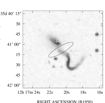
Figure 3: An example of confusing source identification using the NVSS catalog. The IRAS PSC position for IRAS 12173$-$3541 and its error ellipse are centered between the two interacting galaxies while the dominant radio source is identified with the northern galaxy by the NVSS (marked with a white cross).

The distribution of 1.4 GHz radio luminosity for the IRAS 2 Jy sample is shown as a function of galaxy redshifts in Figure 2. Low-luminosity galaxies drop out quickly with increasing redshift due to the IRAS 60 $\mu$m flux cutoff at 2 Jy, but the infrared luminous galaxies are present to $z=0.16$. Therefore, our IRAS 2 Jy sample is not only 6 times larger in the sample size compared with similar previous studies, it also includes sources 5 times further away in the redshift domain as well. The bona fide radio-loud objects in the sample are PKS 1345+12, 3C 273, and NGC 1275, all of which stand out clearly in Figure 2 with $L_{1.4GHz}\geq 1.5\times 10^{25}$ W Hz^-1. Determining the fraction of infrared-luminous objects that are also radio loud (due to the presence of an AGN) is one of the key questions we address later (see §4). One immediate result from this study is the determination of accurate positions for the IRAS Redshift Survey sources. The positions of IRAS sources such as found in the IRAS Point Source Catalog are only accurate to about 15″ (1$\sigma$). In comparison, the source coordinates given by the NVSS catalog have $\sim 1^{\prime\prime}$ rms uncertainties, sufficient for a secure identification of the sources even in a crowded or confused field. For example, the IRAS position error ellipse for the interacting pair IRAS 12173$-$3514 falls between the two widely separated optical galaxies (see Figure 3) while the NVSS catalog identifies the northern galaxy as the dominant source.

The histogram of position offsets between the IRAS PSC and NVSS (Figure 4) shows that the position offset is less than 10″ in over 2/3 of all cases, and this is consistent with the expectation from the IRAS position error.

3 Radio-FIR Correlation

The correlation between the radio and FIR luminosity in galaxies is one of the tightest and best-studied in astrophysics. It holds over five orders of magnitude in luminosity (Price & Duric, 1992), and its nearly linear nature is interpreted as a direct relationship between star formation and cosmic-ray production (Harwit & Pacini, 1975; Rickard & Harvey, 1984; de Jong et al., 1985; Helou et al., 1985; Wunderlich & Klein, 1988).

Evidence for non-linearity in this relation was discussed by Fitt, Alexander, & Cox (1988) and Cox et al. (1988) for magnitude-limited samples of spiral galaxies. Price & Duric (1992) later showed that radio emission can be separated into free-free and synchrotron emission and suggested that the latter causes a greater than unity slope at lower frequencies.

3.1 Observed Radio-FIR Correlation

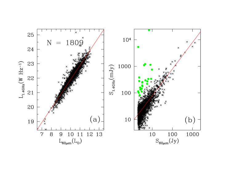
Figure 5: (a) Plot of 1.4 GHz radio luminosity versus IRAS 60 $\mu$m luminosity. The solid line corresponds to a linear relation with a constant offset. (b) Plot of 1.4 GHz and IRAS 60 $\mu$m flux density for the IRAS 2 Jy sample. The solid line corresponds to the same linear relation shown in (a). Gray filled circles identify the radio-excess objects (see §4.2). The remaining $\sim$1750 objects (out of 1809) lie very close to the linear relation, and the rms scatter of the data is less than 0.26 in dex.

The plot of 1.4 GHz radio luminosity versus 60 $\mu$m FIR luminosity for our IRAS 2 Jy sample galaxies (Figure 5a) shows a nearly linear correlation spanning over 5 decades in luminosity. The three noteworthy features are: (1) a unity slope; (2) steepening of the relation at low luminosity ($L_{60\mu m}\leq 10^{9}L_{\odot}$); and (3) a higher dispersion for luminosities above $L_{60\mu m}\geq 10^{10.5}L_{\odot}$.

A formal fit to the observed radio-FIR luminosity correlation yields

$$log(L_{1.4GHz})=[0.99\pm 0.01]log(L_{60\mu m}/L_{\odot})+[12.07\pm 0.08].$$

The overall trend is indistinguishable from a pure linear relation since the overwhelming majority of FIR-selected galaxies have $L_{60\mu m}$ between $10^{9-11.5}L_{\odot}$. The observed strong correlation is accentuated by the distance effect, but the plot of the observed radio and 60 $\mu$m fluxes (Figure 5b) also shows a linear trend spanning nearly three orders of magnitude in flux. In both plots, the scatter is about 0.26 in dex.

There is a systematic tendency of galaxies with $L_{60\mu m}\leq 10^{9}L_{\odot}$ to appear below the best-fit line in Figure 5a, and the diminished radio emission of these galaxies may contribute to the previously reported “non-linear” trend in the radio-FIR relation among optically selected galaxy samples (e.g. Condon et al. 1991a). Such a deviation from the linear relation can occur if the FIR or radio luminosity is not directly proportional to the star forming activity. Dust heating by low mass stars (“cirrus” emission) may contribute only to the observed FIR emission (Helou, 1986; Lonsdale-Persson & Helou, 1987; Fitt, Alexander, & Cox, 1988; Cox et al., 1988; Devereux & Eales, 1989). Alternatively, the radio luminosity of less luminous (and generally less massive) galaxies may be low if cosmic-ray loss by diffusion is important (Klein et al., 1984; Chi & Wolfendale, 1990). Because this sample is FIR selected, there is a potential bias towards sources with higher FIR/radio flux density ratios (see Condon & Broderick 1986). On the other hand, low FIR luminosity sources with relatively high FIR/radio ratios may be missed systematically, possibly offsetting the first potential bias.

3.2 Deviation from the Linear Relation

The presence of any non-linearity or any increase in the dispersion of the radio-FIR correlation may be seen more easily by examining the “$q$” parameter (Condon et al. 1991a),

$$q\equiv log[{{FIR}\over{3.75\times 10^{12}{\rm W~{}m}^{-2}}}]-log[{{S_{1.4GHz}}\over{{\rm W~{}m}^{-2}{\rm Hz}^{-1}}}]$$

where $S_{1.4GHz}$ is the observed 1.4 GHz flux density in units of W m^-2 Hz^-1 and

$$FIR\equiv 1.26\times 10^{-14}(2.58S_{60\mu m}+S_{100\mu m})~{}{\rm W~{}m}^{-2},$$

where $S_{60\mu m}$ and $S_{100\mu m}$ are IRAS 60 $\mu$m and 100 $\mu$m band flux density in Jy (see Helou et al. 1988). Therefore $q$ is a measure of the logarithmic FIR/radio flux-density ratio. For most galaxies in the IRAS Bright Galaxy Sample $q\approx 2.35$, but some galaxies have smaller $q$ values due to an additional contribution from compact radio cores and radio jets/lobes (Sanders & Mirabel, 1996). Optically selected starburst galaxies (interacting/Markarian galaxies) have about the same $q$ values as normal galaxies, and the radio-FIR flux ratio appears to be independent of starburst strength (e.g. Lisenfeld, Volk, & Xu 1996).

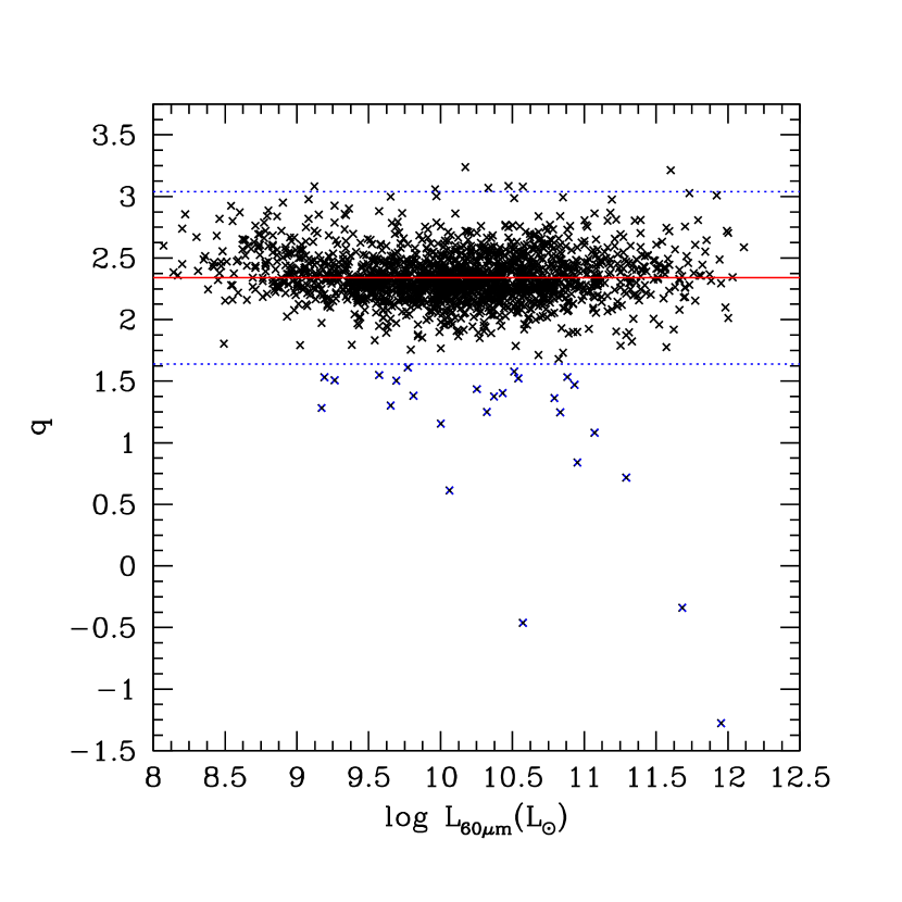
Figure 6: Distribution of $q$ values plotted as a function of IRAS 60 $\mu$m luminosity. The solid line marks the average value of $q=2.34$ while the dotted lines delineate the “radio-excess” (below) and “infrared-excess” (above) objects, delineated for having 5 times larger radio and infrared flux density than the expected values from the linear radio-FIR relation, respectively.

The $q$ values for the IRAS 2 Jy sample were computed using Eq. 5 and are shown in Figure 6. The mean $q$ value for the entire sample is $2.34\pm 0.01$, which is in good agreement with $q$ values typically found in other star-forming galaxies. In fact, the 98% of galaxies in our IRAS 2 Jy sample are found between the two dotted lines which mark the five times excess and deficit of radio emission with respect to mean $q=2.34$ (solid horizontal line).

The effects of measurement errors and source confusion can be estimated from the dispersion in the $q$ value in Figure 6. Before the radio fluxes for galaxies with large angular extent were corrected using the measurements by Condon (1987), several objects with unusually large $q$ values ($q\geq 3$) were found – resulting from the missing extended flux. One object, NGC 5195, also turned out to include incorrect IRAS fluxes in the IRAS redshift catalog, confused with its brighter companion M51. Using the correct IRAS fluxes, its $q=2.68$ became much closer to the sample mean value. Similarly, IRAS 02483+4302 is a well known quasar-galaxy pair and another case of source confusion. Its 1.4 GHz flux was corrected using the measurement by Crawford et al. (1996). These occurrences are consistent with the expected source confusion statistics discussed earlier (§2.3). The direct comparison of Figure 6 with a similar plot in Condon et al. (1991a) suggests that the measurement errors and confusion effects are nevertheless small and comparable to those of the bright spiral sample and the IRAS BGS sample analyzed by Condon et al.

There are good reasons to believe that galaxies with much larger or smaller $q$ values are inherently different. Firstly, there are several objects whose smaller $q$ values are the result of significant excess radio emission associated with AGNs (see §4 for a further discussion). There are also a few infrared-excess objects which may be highly obscured compact starbursts or dust enshrouded AGNs (see §6.1 & §6.2), and some of the observed dispersion may arise at least in part from the variation in excitation or dispersion in dust temperature. The clustering of low-luminosity galaxies ($L_{60\mu m}\mathrel{\hbox{\raise 2.15277pt\hbox{$<$}\hbox to0.0pt{\hss\lower 2.15277pt\hbox{$\sim$}}}}10^{9}~{}L_{\odot}$) above the mean $q=2.34$ in Figure 6 is another clue that the scatter in the $q$ distribution is more than simply statistical in nature. This stems from the previously noted deviation from the linear radio-FIR relation (§3.1), and it is also the source of a small gradient in $q$ noted by Condon et al., due to a systematic decrease in radio emission among low luminosity galaxies. Lastly, the dispersion in the $q$ values among the objects with $L_{60\mu m}>10^{11}L_{\odot}$ is significantly larger, $\sigma_{q}=0.33$. This larger scatter also manifests itself in Figure 6 as the disappearance of the dense core in the distribution near the mean. Helou et al. (1985) noted a similar increase in dispersion at high luminosity in their analysis of only 38 spiral galaxies and suggested that the radio-FIR correlation may break down for high luminosity sources. The new data suggest that the correlation still holds but the dispersion is indeed increased (see below for possible explanations).

4 Radio-Loud and Radio-Excess Galaxies

Two different functional definitions of “radio-loud” objects are found in the literature: one based on absolute radio power and the second based on a relative flux ratio (e.g. $L_{radio}/L_{opt}$). The former are generally a subset of the latter. Here we call “radio-loud” only those galaxies hosting radio sources with $L_{1.4GHz}\geq 10^{25}$ W Hz^-1. In contrast, we define “radio-excess” objects as galaxies whose radio luminosity is five times the value predicted by the radio-FIR correlation or larger (below the lower dotted line in Fig. 6, i.e. $q\leq 1.64$).

4.1 Radio-Loud Objects

It is clear from Figure 2 that there are only three radio-loud objects in our sample of 1809 galaxies, with several others approaching the radio-loud limit. Regardless of the exact statistics, the bona fide radio-loud galaxies are extremely rare among the infrared selected sample. We discuss below the three radio-loud objects in our original sample in detail. It appears that each object represents a special case, and their radio and FIR emission have physically distinct origins.

PKS 1226+023 (3C 273) is a well-known QSO at $z=0.158$ (Schmidt 1963). It is a warm IRAS source ($S_{60\mu m}/S_{100\mu m}=0.76$, $T_{dust}\sim 44$ K) and also the most luminous (log $L_{1.4GHz}=27.42$ W Hz^-1) radio source in our sample. Its elliptical host is somewhat brighter than the brightest galaxy in a rich cluster ($M_{V}=-22.1$, Bahcall et al. 1997) and is probably located inside a poor cluster (Stockton 1980). The large-scale radio structure from the VLA and MERLIN shows a compact, flat-spectrum core and a single jet extending about 23^′′ from the core at a position angle of 222^∘ (Conway et al. 1993). Unlike the other two radio-loud objects discussed below, its infrared emission appears to be mostly the continuation of the non-thermal spectrum from optical to radio wavelengths, associated directly with the AGN.

NGC 1275 (3C 84) is the central giant elliptical galaxy of the Perseus Cluster with a Seyfert 2 nucleus and may be accreting gas from the X-ray emitting intercluster medium via a cooling flow (Kent & Sargent, 1979; Fabian et al., 1981). The bulk of its 1.4 GHz radio continuum emission (log $L_{1.4GHz}=25.13$ W Hz^-1) comes from the core component less than 1″ in size, but it also has a 10′ size extended radio structure that may be interpreted as an asymmetrical Fanaroff-Riley type I source whose jet axis lies close to the line-of-sight (Miley & Perola, 1975; Pedlar et al., 1990). The FIR emission is attributed to an extended ($\sim 30^{\prime\prime}$) distribution of dust, possibly from a kpc scale circumnuclear gas/dust structure accreted from a cluster interloper (Lester et al., 1995; Inoue et al., 1996). Unlike the compact nuclear radio source, the 100 $\mu$m emission in NGC 1275 shows little evidence for variability (Lester et al., 1995). Therefore, the FIR emission in NGC 1275 may be unrelated to the radio emission, which is dominated by the non-thermal emission from the AGN.

PKS 1345+12 (4C 12.50) is the second most luminous radio source in our sample (log $L_{1.4GHz}=26.18$). The optical galaxy has a double nucleus embedded in a distorted halo $\sim 85$ kpc in diameter, indicating a merger system approaching the appearance of a cD galaxy (Mirabel et al., 1989; Shaw, Tzioumis, & Pedlar, 1992). This galaxy has a core-halo radio structure, and more than 95% of the flux at 2 cm wavelength is coming from a region smaller than $0^{\prime\prime}.05$ (106 pc; van Breugel et al. 1984). The western nucleus shows a Seyfert 2 spectrum (Gilmore & Shaw, 1986), and Veilleux et al. (1997) reported broad infrared recombination lines indicative of a hidden QSO. The eastern nucleus is associated with a compact steep-spectrum radio source with a double-lobe structure (Shaw et al. 1992). The large infrared luminosity (log $L_{FIR}(L_{\odot})=11.9$) makes it a genuine ultraluminous infrared galaxy with an extremely large gas content inferred from the CO observations ($M_{H_{2}}=6.5\times 10^{10}~{}M_{\odot}$; Mirabel et al. 1989, Evans et al 1999). Therefore it is one of the best candidates for studying a possible common origin for ultraluminous galaxies and powerful radio galaxies.

4.2 Radio-Excess Objects

One of the key objectives of this study is a quantitative analysis of the frequency and energetic importance of AGNs in FIR-selected galaxies. Assuming that radio excess is an AGN indicator, a total of 23 potential AGN hosts with $q\leq 1.64$ are identified in our sample (see Table 2). The low frequency (23/1809 = 1.3%) of these radio-excess objects indicates that radio AGNs occur quite rarely among the infrared selected sample of normal and starburst galaxies. Among the FIR-luminous galaxies with log $L_{FIR}\geq 11.3L_{\odot}$ listed in Table 1, there are only three radio-excess galaxies (IRAS 12173$-$3541, IRAS 12265+0219, IRAS 13451+1232). This fraction, 3/161 = 1.9%, is only marginally larger than the radio-excess fraction among the entire IRAS selected sample. Therefore the radio-excess fraction is generally only a few percent and is nearly independent of the infrared luminosity.

How does this result compare with the analysis of optically selected galaxy samples? Condon & Broderick (1988) have identified a total of 176 radio sources with $S_{1.4GHz}\geq 150$ mJy among galaxies in Uppsala General Catalogue of Galaxies (Nilson 1973; hereafter UGC). Judging by the radio morphology, radio-to-infrared flux density ratio, and infrared spectral index, 64 are identified as “starbursts” and 103 (59%) are identified as “monsters”. There are four borderline cases while no infrared data are available for the remaining three. We find that the same distinctions could have been made using their radio-to-FIR flux ratio alone. Among the “monsters” in the UGC sample, only 6 galaxies (UGC 2188, 2669, 3374, 3426, 8850, and 12608) are bright enough at 60 $\mu$m to be included in our sample, and all but UGC 2188 are identified as radio-excess by our analysis. The starburst/Seyfert galaxy UGC 2188 (NGC 1068) has $q=1.72$ and is also marginally radio-excess (about 4 times larger radio luminosity than expected from the radio-FIR correlation). Therefore there is little overlap between the “monsters” in the UGC sample and our IRAS 2 Jy sample. This is mainly due to the relatively large radio flux cutoff used in the UGC study, which has introduced a strong bias in favor of radio bright AGNs. As the radio flux cutoff is lowered, the dominance of the star-forming galaxies emerges quickly as shown by the preliminary analysis of the UGC galaxies using the NVSS database (Cotton & Condon, 1998). The relative frequencies of “monsters” and star-forming galaxies is addressed further in terms of their luminosity functions below.

The frequency of radio-excess objects derived above is strictly a lower limit to the overall frequency of AGNs among the IR selected galaxies. Radio luminosity of AGNs ranges over 10 orders of magnitudes (e.g. Condon & Broderick 1988, Ho & Ulvestad 2000), and radio-quiet AGNs might not be that rare in our sample. Nevertheless a large majority of luminous AGNs are radio sources and may be readily identified. For example, 84% (96/114) of Palomar Bright Quasar Survey sources have been detected by Kellermann et al. (1989) at 5 GHz using the VLA. Evidence for radio emission in excess of the inferred star formation activity level among high redshift dusty, radio-quiet QSOs has also been discussed by Yun et al. (2000). To quantify the robustness of radio-excess as an AGN indicator, we have examined the radio properties of a sample of 48 Palomar-Green (PG) survey QSOs with IRAS detections reported by Sanders et al. (1989). Ten of these sources were dropped from our analysis, either because the XSCANPI analysis revealed the IRAS detections to be the results of confusion or because meaningful upper limits for the FIR and radio luminosity could not be obtained. Among the remaining 38 PG QSOs, only 23 have $L_{60\mu m}>10^{11}L_{\odot}$. The radio-excess fraction among this subsample of FIR luminous QSOs is 12/23=52%, which greatly exceeds the frequency for our IRAS selected galaxy sample (see above). Among the remaining 11 PG QSOs without the excess radio emission, Alloin et al. (1992) detected CO emission with inferred molecular gas mass larger than $10^{10}M_{\odot}$ in all three objects observed and argued that star formation may be responsible for the bulk of the FIR luminosity among these QSOs. Therefore the overall frequency of AGNs may be somewhat larger than inferred from the radio-excess alone – perhaps as much as twice as large in the case of the IRAS selected PG QSOs. Further discussions of the frequency of energetically dominant AGNs are found in the Discussion section (§6), including the examination of the mid-infrared properties.

5 Radio and Far-infrared Luminosity Functions

With 1809 galaxies in our IRAS 60 $\mu$m flux-limited sample, we should be able to derive the radio and FIR luminosity functions (LFs) for field galaxies in the local volume with significantly better statistics than previously possible. Since our sample covers a significantly larger solid angle and volume than the samples used previously, fluctuations produced by large-scale structures and clustering should be smaller. If there is a significant presence of radio AGNs contributing to our IRAS selected sample, not only they can be identified as a separate population in the derived radio and/or FIR luminosity functions, we can also determine the range of luminosity where their contribution is significant.

Several different functional forms have been suggested previously for the radio and FIR luminosity functions of field galaxies, such as log-normal (Hummel, 1981; Isobe & Feigelson, 1992), hyperbolic (Condon, 1984), two power-laws (Soifer et al., 1987), and power law/Gaussian (Sandage et al., 1979; Saunders et al., 1990). These functional forms offer reasonable descriptions of the observed radio and FIR LFs with varying degrees of relative merit. All previously published studies, however, have unanimously rejected the traditional form proposed by Schechter (1976) as being too narrow to describe the observed radio or FIR LFs. This is surprising because Schechter function offers an excellent and robust description of the optical LFs of field galaxies and galaxy clusters (e.g. Shapiro 1971, Schechter 1976, Auriemma et al. 1977, Efstathiou, Ellis, & Peterson 1988). Extinction effects at optical wavelengths cannot explain this discrepancy because Schechter function also offers an excellent description of near-IR LFs of galaxies (Gardner et al., 1997; Szokoly et al., 1998; Loveday, 2000). Therefore the failure of the Schechter form is highly unusual and deserves further investigation.

5.1 Schechter Luminosity Function

Here we revisit the idea of describing the observed radio and FIR LFs in terms of Schechter functions for two important reasons. First, the Schechter function has a simple but sound theoretical basis as it follows from a theoretical analysis of self-similar gravitational condensation in the early universe (Press & Schechter, 1974). The Schechter function has a form

$$\rho(L)dL=\rho^{*}(L/L^{*})^{\alpha}\exp(-L/L^{*})d(L/L^{*})$$

where $\rho^{*}$ and $L^{*}$ are the characteristic density and luminosity of the population, and $\alpha$ describes the faint-end power-law slope for $L\ll L^{*}$ (Schechter 1976). Not only is the Press-Schechter formalism a well accepted paradigm for cosmological structure formation, but the Schechter function also describes the observed optical and near-IR LFs of field and cluster galaxies well as already mentioned. If star formation activity is an integral part of galaxy evolution and reflects the nature of the host galaxies, then the Schechter function should also offer a good description for the radio and FIR LFs as it does for the optical and near-IR LFs.

Another reason for reconsidering the Schechter form is that the observed departure, namely the power-law tail at high luminosity end for the FIR LF, may have been a predictable consequence of the underlying theoretical consideration in the Press-Schechter formalism. To be specific, the Press-Schechter formalism for CDM structure formation predicts a mass function of the Schechter form, rather than a luminosity function. To make the logical connection between the observed LFs and the Press-Schechter formalism, one has to invoke a constant mass-to-light (M/L) ratio, which is a reasonable assumption at the optical and near infrared wavelengths. For starburst galaxies, on the other hand, a momentary jump in L/M by 2-3 orders of magnitudes is expected by definition, nearly entirely at the FIR wavelengths. Therefore, if the underlying mass distribution is of a Schechter form, the resulting FIR (and radio) LF should be a linear combination of a Schechter function (for field galaxies) and a high luminosity excess due to starburst galaxies. Hence, we pose a hypothesis that the observed radio and FIR LFs are indeed linear sums of two Schechter functions, one for the field galaxies and second for the starburst population. Choosing a Schechter form for the starburst population is largely for self-consistency. If this population is distinguished only by 2-3 orders of magnitude elevation in M/L, then a Schechter function should also represent a reasonable form for its LF. We examine this hypothesis by analyzing the derived radio and FIR LFs in detail below.

The characteristic Schechter parameters for the observed LFs are derived in two different ways. A luminosity function is the space density of the sample galaxies within a luminosity interval of $\Delta L$ centered on $L$. Thus the LF and associated uncertainty can then be derived “directly” as

$$\rho_{m}(L)=\sum_{i=1}^{N}({{1}\over{V_{m}}}),~{}~{}~{}\sigma_{\rho(L)}=(\sum_{i=1}^{N}{{1}\over{V_{m}^{2}}})^{1/2}$$

where $\rho_{m}(L)$ is the measured luminosity density within the “magnitude” bin centered on luminosity $L$ and $V_{m}$ is the sample volume appropriate for each of the N=1809 galaxies (Schmidt, 1968; Felten, 1976). The sample volume $V_{m}$ was determined by the IRAS 60 $\mu$m sensitivity limit of 2 Jy and the NVSS survey area as:

$$\int_{0}^{D}r^{2}dr\int_{0}^{2\pi}d\rho\int_{\delta=-40^{\circ}}^{\delta=+90\circ}\cos\delta d\delta=3.44D^{3}.$$

The sampled volume is further reduced by 18% due to the exclusion of the Galactic Plane and the omitted areas in the IRAS redshift survey.

The Schechter parameters can also be derived from the observed luminosity distribution, $n(L)$. For a randomly chosen sample, the distribution function $n(L)$ is given by

$$n(L)\equiv\rho(L)V(L),$$

where $V(L)$ is the volume sampled. The distribution function can then be re-written as

$$n(L)dL=\rho^{*}V^{*}(L/L^{*})^{\alpha+3/2}exp(-L/L^{*})d(L/L^{*})$$

where $V^{*}$ is the characteristic volume associated with $L^{*}$. Given these analytical expressions for the luminosity distribution and luminosity function, a $\chi^{2}$ analysis is performed on the observed $\rho(L)$ and $n(L)$ to deduce the characteristic Schechter parameters. The Schechter parameters derived from $\rho(L)$ and $n(L)$ are slightly different because the two methods are subject to slightly different systematic effects. In addition to the formal uncertainties given by the $\chi^{2}$ analysis, the difference between the best-fit parameters derived by the two different methods offers a quantitative measure of the systematic errors in the derivations.

A potential source of confusion in comparing the derived LFs from one study to another is the definition of luminosity interval $\Delta L$ used. Both “per magnitude” and “per dex” are commonly used in the literature. We adopt “per magnitude (mag^-1)” in our derivations of radio and FIR luminosity functions. All published luminosity functions using “dex^-1” intervals (e.g. Saunders et al. 1990) are thus corrected by a factor of 2.5 before making any comparisons.

5.2 IRAS 60 $\mu$m Luminosity Function

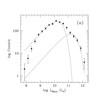
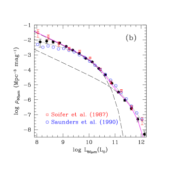
Figure 7: (a) 60 $\mu$m luminosity distribution for the IRAS 2 Jy sample. The data points are number of counts in each luminosity bin, and the error bars reflect the Poisson statistics, $N^{1/2}$ (see Table 4). The two solid lines indicate the best-fit curves of the Schechter form listed in Table 5. (b) The $60\mu$m infrared luminosity function. Filled circles represent the LF for the IRAS 2 Jy sample. The open squares and open circles represent the 60 $\mu$m LFs derived from the IRAS BGS sample by Soifer et al. (1987) and an ensemble of data (“S17”) analyzed by Saunders et al. (1990), respectively. The long dashed lines correspond to the two Schechter fits for the high and low luminosity objects listed in Table 5. The solid line is the resulting linear sum of the two Schechter functions. The dotted curve represents the double power-law LF derived from an earlier version of the IRAS redshift survey sample by Yahil et al. (1991) using a density-independent determination method. (c) The $V/V_{m}$ plot for the IRAS $60\mu$m luminosity distribution. The $V/V_{m}$ analysis suggests that the highest and the lowest luminosity bins are not well sampled and may suffer a completeness problem.

The IRAS 60 $\mu$m luminosity distribution and luminosity function for the IRAS 2 Jy sample galaxies are constructed using 18 luminosity bins of log $L_{60\mu m}$ ($L_{\odot}$) between 7.75 and 12.25 with a width of $\Delta\log L=0.25$. The computed 60 $\mu$m luminosity distribution and LF are tabulated in Table 4 along with the computed $V/V_{m}$, which is a measure of the sampling completeness (Schmidt, 1968; Felten, 1976). These quantities are also shown graphically in Figure 7 along with the best-fit Schechter functions (see below). The luminosity distribution shown in Figure 7a nicely indicates that the most common objects in the IRAS 2 Jy sample have 60 $\mu$m luminosity of about $10^{10}L_{\odot}$, typical of $L^{*}$ galaxies in the field.

The derived 60 $\mu$m LF is shown in Figure 7b and is compared with previous derivations by Soifer et al. (1987) and Saunders et al. (1990). The general shape of the LF may be reasonably described as a power-law distribution, but two or more power-laws are needed to account for the detailed shape in the entire luminosity range. As discussed in the previous section (§ 5.1), a linear sum of two Schechter functions may make a good physical sense as a description for the radio and FIR luminosity functions, and indeed the derived analytical expressions shown in the solid and dashed lines match the the observed 60 $\mu$m LF closely. In deriving the best fit Schechter parameters, the faint end power-law slope $\alpha$ is assumed to be universal because it cannot be derived cleanly for the higher luminosity (“starburst”) population. The characteristic luminosities $L^{*}$ derived from the 60 $\mu$m luminosity distribution (Figure 7a) for the high- and low-luminosity populations are $(21\pm 2)\times 10^{10}L_{\odot}$ and $(2.2\pm 0.4)\times 10^{10}L_{\odot}$, respectively, with the faint end power-law slope $\alpha=-0.81\pm 0.06$. The best fit parameters can also be derived from the observed 60 $\mu$m luminosity functions (Figure 7b), and they are $(22\pm 2)\times 10^{10}L_{\odot}$ and $(2.3\pm 0.5)\times 10^{10}L_{\odot}$, with $\alpha=-0.82\pm 0.05$ (see Table 5 for the summary and the ${\chi}^{2}$ analysis).

A break in the FIR LF has previously been suggested by Smith et al. (1987) and Saunders et al. (1990) based on the optical morphology and infrared color. These authors had not offered any clear physical explanations for such a break seen near $L_{60\mu m}=10^{11}L_{\odot}$, however. The combination of an even cleaner break seen in the 1.4 GHz radio LF (see below) and the excellent fits reported in Table 5 lend strong support for the two Schechter function description and the implied physical explanation in terms of an elevated mass-to-light ratio for the starburst population.

Significant differences are seen among the several 60 $\mu$m LFs compared in Figure 7b at the low luminosity end. Our 60 $\mu$m LF (filled circles) is smoother and has smaller error bars than those derived by Soifer et al. (1987) and by Saunders et al. (1990) because our sample size is 6 times larger. Our 60 $\mu$m LF dips below the Soifer et al. LF (empty squares) and the derived Schechter model near $L_{60\mu m}\mathrel{\hbox{\raise 2.15277pt\hbox{$<$}\hbox to0.0pt{\hss\lower 2.15277pt\hbox{$\sim$}}}}10^{8.5}L_{\odot}$. The 60 $\mu$m LF derived by Saunders et al. (1990; empty circles) flattens even further, beginning around log $L_{60\mu m}\sim 9.5$. This flattening is also seen in their Figure 2, in comparison with that of BGS sample (Soifer et al. 1987), Smith 2 Jy sample (Smith et al. 1987), and Strauss & Huchra (1988). One explanation for the different faint end slope may be the sample completeness as the surveys with particular emphasis on the completeness (e.g. Smith et al., Stauss & Huchra) tend to derive a steeper faint end slope. In contrast, Saunders et al. data probably suffers the worse completeness problem because their luminosity function is derived using a heterogeneous collection of several different surveys. The plot of $V/V_{m}$ (Fig. 7c) shows that our sample is distributed fairly uniformly within the sampling volume ($V/V_{m}\sim 0.5$).

The derived $V/V_{m}$ for our sample dips below 0.5 at log $L_{60\mu m}\mathrel{\hbox{\raise 2.15277pt\hbox{$<$}\hbox to0.0pt{\hss\lower 2.15277pt\hbox{$\sim$}}}}8.5$, albeit with large errorbars. This can be interpreted as an indication of local density enhancement and may be reflecting our special location within the local galaxy group and the local super-cluster. Derivation of LFs using the $1/V_{m}$ method (Eq. 8) has been suggested to be susceptible to the large scale inhomogeneity, and the steep rise in the derived LF at the faint end may be an artifact of this bias. The steepest rise in the faint end slope is associated with the LF derived by Soifer et al. which also has the smallest sampling volume, in accordance with this expectation. Assuming the luminosity function has a universal form, Yahil et al. (1991) proposed a density-independent determination of the luminosity function by introducing a selection function which accounts for the distance effect. The Yahil et al. derivation of a double power-law form LF using an earlier version of the IRAS redshift catalog is shown as a dotted curve in Figure 7b. While the derived faint end slope is flatter and shallower than the LF we derive, it is also steeper and higher than the LF derived by Saunders et al. (also see their Fig. 7). Even such a density-independent method faces a fundamental limitation if the faint end slope is constrained by the low luminosity objects that are drawn mainly from the local volume with enhanced density. Therefore the analysis presented here suggests that the faint end behavior of the luminosity function is intrinsically poorly constrained. It should be noted, however, that these differences between the various LFs at low L do not have much effect on the implied star formation density discussed below (§6.4) since the star-formation rate is proportional to the LF multiplied by L, a function peaking at higher luminosity.

5.3 1.4 GHz Radio Luminosity Function

Because our sample is selected by the IRAS 60 $\mu$m band flux density, deriving the 1.4 GHz radio luminosity function for the same sample is not as straight forward as in the 60 $\mu$m LF case. In particular, the 1.4 GHz radio LF cannot be derived from the luminosity distribution (Eq. 11) because the volume sampled does not relate directly to the 1.4 GHz luminosity. Instead, the 1.4 GHz radio luminosity function is derived using the sampling volume corresponding to the IRAS 60 $\mu$m luminosity of each sample galaxy. The logic behind this calculation is that each sample galaxy contributes to the local number density at their respective luminosity bins in exactly the same manner for both the 60 $\mu$m and 1.4 GHz LF, and sample selection is reflected identically by the sample volume determined by the IRAS 60 $\mu$m flux limit.

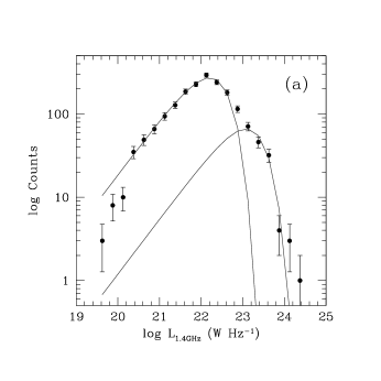
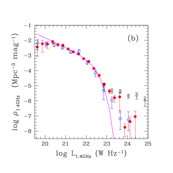
Figure 8: (a) 1.4 GHz radio luminosity distribution for the IRAS 2 Jy sample. The data points are number counts in each luminosity bin, and the error bars reflect the Poisson statistics, $N^{1/2}$ (see Table 6). The two solid lines indicate the best-fit curves of the Schechter form listed in Table 7. (b) The 1.4 GHz radio luminosity function. Filled circles represent the IRAS 2 Jy sample while the open circles and squares represent the 1.4 GHz LFs for the “starburst” and “monsters” from Condon (1989), respectively. The solid line is the best fit Schechter function for the low luminosity objects only (see Table 7). (c) The $V/V_{m}$ plot for the 1.4 GHz radio luminosity distribution. The error bars are statistical and may not be accurate for bins with small number of counts. The $V/V_{m}$ analysis suggests that the highest and the lowest luminosity bins are not well sampled and may suffer a completeness problem.

The computed radio luminosity distribution and LF are tabulated in Table 6 along with the computed $V/V_{m}$. These quantities are also shown graphically in Figure 8 along with the best-fit Schechter functions (see Table 7). The radio luminosity distribution, LF, and the $V/V_{m}$ plots are qualitatively similar to those of the IRAS 60 $\mu$m functions in Figure 7, mainly because of the linear radio-FIR correlation (see §3 & §6.3). The derived 1.4 GHz radio LF, shown in Figure 8b, is flat at low luminosity end and falls off steeply beyond $10^{22}$ W Hz^-1. A Schechter function (solid line) appears to be a good description for all low luminosity objects of $L_{1.4GHz}\leq 10^{23}$ W Hz^-1, with the best fit characteristic Schechter parameters of $L^{*}=(2.1\pm 0.3)\times 10^{22}$ W Hz^-1, $\rho^{*}=(3.2\pm 0.2)\times 10^{-4}$ Mpc^-3 mag^-1, and $\alpha=-0.63\pm 0.05$. The observed radio LF is significantly flatter than the best fit Schechter function below $L_{1.4GHz}\leq 10^{20.4}$ W Hz^-1. In addition to the possible effects of sample completeness and local density enhancement, the systematic deviation from the linear radio-FIR relation may further contribute to this flattening.

The presence of the luminous second population is more obvious in Figure 8b at $L_{1.4GHz}\geq 10^{23}$ W Hz^-1. A full $\chi^{2}$ analysis is not warranted for this population because of the small numbers of bins represented and the large observed scatter. Characteristic luminosity and density of $L^{*}=(1.4\pm 0.2)\times 10^{23}$ W Hz^-1 and $\rho^{*}=(8.3\pm 0.8)\times 10^{-6}$ Mpc^-3 mag^-1 are derived assuming the same faint-end power law slope of $\alpha=-0.63$, but these numbers should be taken only as illustrative values. The flux cutoff of 2 Jy at 60 $\mu$m and the resulting volume sampled are probably not sufficient to fairly represent these rarest objects with high luminosity.

The comparison of our radio LF (filled circles) with that of the flux limited sample of UGC galaxies by Condon (1989; open circles) shows that the low radio luminosity galaxies in our IRAS selected sample are nearly identical to the “starburst” galaxies (late type galaxies in the field, as opposed to “monsters”) in the UGC catalog (see Figure 8b). The small excess associated with the IRAS 2 Jy sample is entirely accounted by the cluster galaxy population. When all galaxies within the 3 Mpc projected diameter of the known clusters within 100 Mpc distance are removed, the resulting radio LF is indistinguishable from the UGC sample LF. The significance of this result is that there is a complete overlap between the optically selected late type galaxies and IRAS selected galaxies in the field. In other words, the measured radio luminosity may be used to infer star-forming activity for late-type galaxies in the field with the same level of confidence as using their FIR luminosity. Estimating the star-formation rate for an individual galaxy using its radio luminosity may still be uncertain by the magnitude of the observed scatter in Figure 6, but such an analysis for an ensemble of galaxies should be significantly more reliable (see §6.5).

The comparison with the “monsters” in the UGC sample (open squares), which has a flat luminosity function, is more complicated. The 1.4 GHz radio LF for the “monsters” derived by Condon is comparable to that of our IRAS selected galaxy sample for $L_{1.4GHz}$ between $10^{23}$ and $10^{24}$ W Hz^-1, but the difference quickly grows to more than an order of magnitude at $L_{1.4GHz}\mathrel{\hbox{\raise 2.15277pt\hbox{$>$}\hbox to0.0pt{\hss\lower 2.15277pt\hbox{$\sim$}}}}10^{24}$ W Hz^-1. This disagreement at the highest luminosity is highly statistically significant, and it must be explained by the incompleteness in the IRAS 2 Jy sample. The LF of galaxies is a property of galaxies and not of the sample; the $1/V_{m}$ weighting is supposed to correct for sample selection effects. With a sufficiently large sample of IRAS galaxies, the LF should equal the LF of optical/radio selected UGC galaxies, including both starbursts and monsters. The main reason that our IRAS total LF is lower than the UGC monster LF must be that NO “monsters” have been detected by IRAS in the highest luminosity bins. If even one or two were detected, they would have small $V_{m}$ values and hence large weights, bringing up the IRAS LF to agree with the UGC LF. Therefore, the second, more luminous population in the IRAS 2 Jy sample cannot be simply identified with the “monsters” in the UGC sample. Because these high luminosity objects also largely follow the same radio-FIR correlation as the low luminosity objects (see Fig. 5), the observation can be explained more naturally with our hypothesis that the high-luminosity excess represents a physically distinct second population, whose large luminosity is the manifestation of a burst of tidally or merger induced activities (see § 5.1). Possible contribution by luminous AGNs are discussed in greater detail below.

6 Discussion

6.1 High Luminosity Objects and Frequency of AGNs

Infrared-luminous galaxies with $L_{FIR}\geq 10^{11}~{}L_{\odot}$ (equivalently, $L_{1.4GHz}\geq 10^{23}$ W Hz^-1) are special objects because few normal disk galaxies in the local universe have such large luminosity. A complete list of 161 luminous infrared galaxies with $L_{60\mu}\geq 10^{11.3}L_{\odot}$ is given in Table 1. In addition to many well-known ultraluminous infrared galaxies (e.g. Arp 220), Seyferts, starburst, and HII galaxies are included in the list, and morphological descriptions of “interacting”, “galaxy pairs”, or “mergers” are common. More importantly, they may represent a distinct separate population from the late type field galaxies in the derived radio and FIR LFs (see §5).

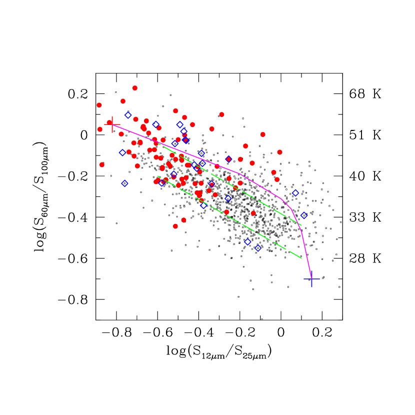
Figure 9: IRAS mid-IR to far-IR color-color diagram for our IRAS 2 Jy Sample. Large filled circles correspond to infrared luminous galaxies with $L_{60\mu}\geq 10^{11.3}L_{\odot}$ (see Table 1). The low luminosity, late type galaxies in the field are plotted in small dots. The large diamonds identify the “radio-excess” objects (radio AGNs; Table 2). The twin broken parallel lines trace the area occupied by “normal galaxies” as identified by Helou (1986), and the curved solid line is the theoretical trajectory of mixed composition dust under increasing mean radiation field calculated by Désert (1986), from solar neighborhood intensity (“cirrus”, lower right) to several hundred times larger radiation field (upper left).

The infrared color-color diagrams shown in Figure 9 provide a useful tool for probing the mean radiation field and dust composition. In analyzing the IRAS colors of field galaxies, Helou (1986) found a linear trend of increasing dust temperature with increasing luminosity as shown by the dashed parallel tracks in Figure 9. The high-luminosity objects (filled large circles) as a group show a systematically larger 60 $\mu$m to 100 $\mu$m flux ratio, which is an indication of warmer mean dust temperature ($S_{60\mu m}/S_{100\mu m}\sim 0.8$, $T_{dust}\sim 45$ K). They also cluster near the upper left corner of Figure 9, which indicates that the dust in these galaxies is exposed to hundreds of times stronger radiation field than that of the solar neighborhood. This clustering is broadly consistent with the intense starburst interpretation for these FIR-luminous systems. Even though their FIR luminosity is on average 10 times smaller, the radio-excess objects (radio AGNs, shown as diamonds) show a similar IRAS color distribution as infrared luminous galaxies. An AGN produces its characteristic mid-IR enhancement by heating a small amount of dust in its immediate surroundings to a very high temperature. The observed similarity in the IR color between luminous starbursts and AGNs might indicate that the warm dust heated by stars may also be concentrated in a relatively small volume.

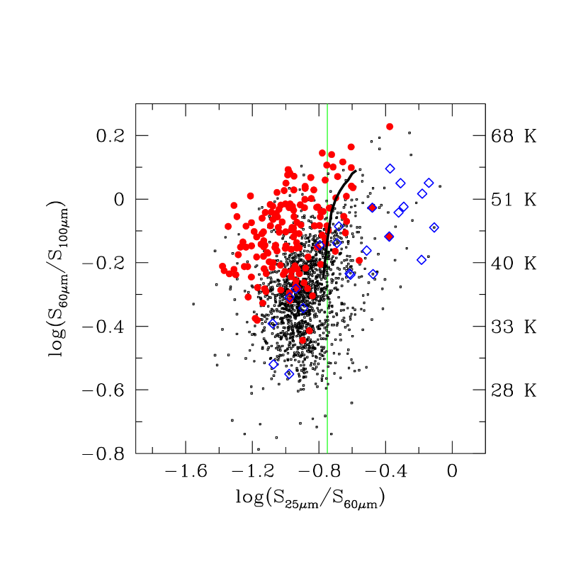
Figure 10: IRAS far-IR versus mid-IR color-color plot for the IRAS 2 Jy sample. The $S_{60\mu m}/S_{100\mu m}$ ratio is translated into dust temperature assuming emissivity index $\beta=1$ (see Helou et al. 1988). All the symbols are the same as in Figure 9. The thin vertical line marks the proposed division for the infrared Seyferts ($S_{25\mu m}/S_{60\mu m}\geq 0.18$) by de Grijp et al. (1985). The thick solid line represents the color evolution track for a model starburst galaxy from Efstathiou et al. (2000), starting at zero age on the top right corner to 72 Myr old starburst at the end (see their Fig. 2 for more detail).

While an unambiguous distinction is not possible, a systematic separation among the late type field galaxies, infrared luminous galaxies, and radio AGNs becomes more apparent in the far-IR versus mid-IR color plot as shown in Figure 10. The far-IR color of the FIR-luminous sample is clearly and systematically warmer than that of the late type field galaxies (small dots). The median $S_{60\mu m}/S_{100\mu m}$ ratio for the FIR-luminous galaxies is about 0.8 (45 K for $\beta=1$; see Helou et al. 1988) while it is about 0.5 (36 K for $\beta=1$) for the field galaxies. The radio-excess objects show a similar range of the far-IR colors as the infrared luminous objects. In addition, they also show a systematic offset towards the warmer mid-IR color by about 0.5 in dex, separating themselves from the infrared luminous galaxies. Presence of hot dust in the circumnuclear region surrounding an AGN offers a plausible explanation for this mid-IR enhancement. Mid-IR excess with $S_{25\mu m}/S_{60\mu m}\geq 0.18$ (right of the thin vertical line) has been empirically proposed as an indicator of an infrared AGN by de Grijp et al. (1985). Indeed the radio-excess objects in our sample show the largest $S_{25\mu m}/S_{60\mu m}$ ratios among all IRAS selected galaxies (see Figure 10).

A total of 20 out of the 161 FIR-luminous objects in our IRAS 2 Jy sample have $S_{25\mu m}/S_{60\mu m}\geq 0.18$. This fraction (20/161=12%) can be interpreted as an upper limit to the fraction of FIR-luminous galaxies that may be powered primarily by an AGN. Genzel et al. (1998) found that an energetically dominant active nucleus is present in 20 to 30% of all FIR-ultraluminous galaxies based on the analysis of their mid-IR diagnostic diagram. This broad agreement is not surprising since both methods utilize the enhanced mid-IR emission as an indicator. The actual fraction of FIR-luminous galaxies powered by AGNs may be smaller still as discussed below. The total fraction of radio-excess objects among the mid-IR excess objects is only 10% (2 out of 20). Perhaps fortuitously, this fraction is similar to the frequency of radio-loud objects among optically identified QSOs (Kellermann et al., 1989; Hooper et al., 1995).

The proposed separation of AGNs from star forming galaxies using the $S_{25\mu m}/S_{60\mu m}$ flux ratio is not entirely supported by Figure 10, however. Both the field galaxies and FIR-luminous galaxies show a broad general trend towards a higher $S_{25\mu m}/S_{60\mu m}$ flux ratio with increasing $S_{60\mu m}/S_{100\mu m}$ flux ratio. This trend is seen more clearly when each class of objects are considered separately, and this follows the expected behavior for an aging and evolving starburst. To quantify this trend, the color evolution track for a starburst galaxy computed by Efstathiou et al. (2000) is shown as a thick curve in Figure 10. In this model, a starburst at its onset (top right end of the track) displays significant mid-IR emission contributed by the hot/warm dust directly exposed to the intense radiation field of the young massive stars. The predicted $S_{25\mu m}/S_{60\mu m}$ ratio is comparable to the largest values observed for the FIR-luminous galaxies. As the starburst ages and the hot/warm dust cools, the starburst travels down along the track as shown in Fig. 10. It is particularly interesting that this color evolution track closely hugs the proposed AGN separation line at $S_{25\mu m}/S_{60\mu m}=0.18$ and outlines the right side boundary for the FIR-luminous objects in this plot. The treatment of the supernova ejecta in this model is such that the evolution track shown is essentially the right boundary for a family of possible evolution tracks, in agreement with the data shown here – see Efstathiou et al. (2000) for a detailed description of the model. The youngest starbursts ($\leq 20$ Myr) are predicted to appear well to the right of the AGN separation line, and this prediction is further supported by the fact that young starburst galaxies hosting massive Wolf-Rayet clusters such as NGC 1614, NGC 1741, and NGC 5253 show Seyfert-like mid-IR excess with $S_{25\mu m}/S_{60\mu m}$ flux ratios of 0.22, 0.15, and 0.39, respectively, while they show no evidence for hosting an AGN. Therefore some caution should be taken for interpreting mid-IR excess as an AGN indicator, especially for galaxies with warm far-IR color.

The fact that an overwhelming majority of high-luminosity objects in our IRAS selected sample do not show mid-IR excess and have the same infrared color characteristics as the less luminous normal star forming galaxies would argue that most of them are powered by an intense starburst instead. The derived radio LF for the high-luminosity objects in the IRAS 2 Jy sample being not consistent with that of the radio AGNs or “monsters” in the UGC sample of Condon (1989) also indicate that the majority of them may not be powered by an AGN. Further, about 30% (7/23) of the radio-excess objects appear to the left of the mid-IR excess line in Figure 10, indicating that some of the radio AGNs do not contribute significantly to their host’s infrared luminosity.

6.2 Nature of FIR-Excess Galaxies

There are nine objects in the IRAS 2 Jy sample with unusually large FIR/radio flux ratios with $q\geq 3$. Three objects have $S_{60\mu m}/S_{100\mu m}>1$ ($T_{d}=60\sim 80$ K), and the dust temperatures in these galaxies are among the highest in the sample. The strong temperature dependence in dust emissivity implies that a dramatic increase in FIR luminosity can result from only a slight increase in dust temperature. Similarly large $S_{60\mu m}/S_{100\mu m}$ ratios are also found in infrared quasars FSC 09105+4108 (Hutchings & Neff, 1988), FSC 13349+2438 (Beichman et al., 1986), FSC 15307+3252 (Cutri et al. 1994) and other luminous AGN host galaxies (see Yun & Scoville 1998). Ironically, broad emission lines indicative of a luminous AGN have not been detected by optical or infrared spectroscopy among the FIR-excess galaxies observed to date. Evidence for large visual extinction and/or large gas and dust contents is present in the four best studied galaxies (NGC 4418, IRAS 08572+3915, IRAS 20087$-$0308, IRAS 22491$-$1808).

Using the high resolution imaging of 8.4 GHz radio emission in the 40 ultraluminous galaxies in the IRAS Bright Galaxy Sample, Condon et al. (1991b) have shown that starburst regions in some of these galaxies are compact and dense enough to be opaque even at mid-IR and long radio wavelengths. Such compact and intense starbursts can indeed account for the large $S_{60\mu m}/S_{100\mu m}$ ratios and high extinction at the same time. These infrared excess objects may actually represent a special phase in the starburst evolution.

The existing data, however, cannot uniquely distinguish whether these FIR-excess objects are powered by a dust enshrouded AGN or by a compact starburst. If a dense environment and associated large opacity is responsible for the observed infrared excess, then one cannot possibly probe the energy source directly since the central active region must be opaque – even for hard X-ray photons if the line of sight column density exceeds $10^{24}$ cm^-2. If free-free absorption is responsible for the low 1.4 GHz flux, then dense ionized gas must fill most of the 1.4 GHz source volume ($>50-100$ pc in size). Since the UV opacity is so high, an ionizing photon cannot travel very far before being absorbed by dust. Thus an extended, distributed source (a starburst) is favored over a single point source (an AGN) to account for the observed ionization.

What is more certain is that such a compact starburst phase or a dust-enshrouded AGN phase must be brief, perhaps only a few percent of the IR bright phase, because only nine out of 1809 sources show such infrared excess. Converting significant fraction of the AGN luminosity into thermal dust emission requires a geometry for thoroughly enshrouding the AGN with dust. The paucity of FIR-excess objects in the IRAS 2 Jy sample thus argues strongly that FIR-luminous galaxies powered by luminous AGNs account for a very small fraction. The AGN-powered FIR-luminous galaxies may be in the radio-excess phase instead, but we have already established in § 4.2 that the radio-excess fraction is less than a few per cent, independent of luminosity.

6.3 Evidence for Non-linearity in the Radio-FIR Correlation

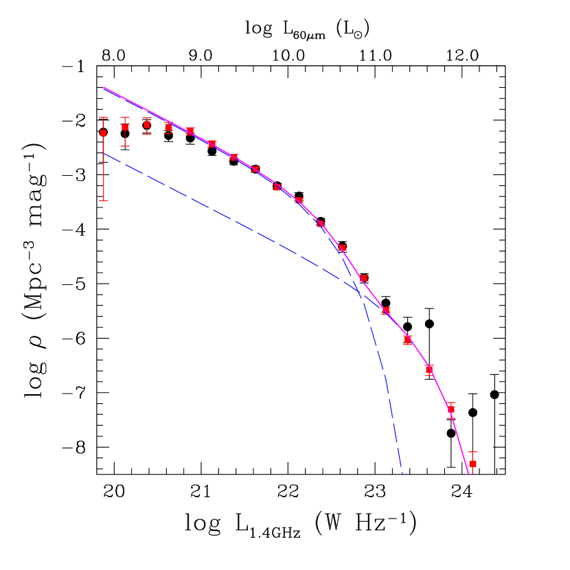
Figure 11: The 60 $\mu$m FIR LF (in filled squares) is translated using the linear radio-FIR relation in Eq. 4 and compared directly with the 1.4 GHz radio LF (in filled circles). The two Schechter functions for the high and low luminosity 60 $\mu$m FIR LFs are shown in long dashed lines and the sum of the two are shown in thick solid line as in Figure 7b.

As a further test of the radio-FIR correlation, the IRAS 60 $\mu$m LF is plotted on top of the 1.4 GHz radio LF in Figure 11 after shifting the 60 $\mu$m LF along the x-axis using the linear radio-FIR relation in Eq. 4. The agreement is extremely good for the two LFs over a wide range of luminosity. A total of 1467 galaxies (81%) belong to the luminosity range between $10^{21}$ and $10^{23}$ W Hz^-1 where the two LFs are essentially identical. The luminosity range over which the two LFs agree within a factor of two includes over 98% of the total sample. Thus, the similarity between the two LFs stems from the fact that the overwhelming majority of galaxies in our IRAS selected sample follow the same linear radio-FIR correlation.

Evidence for diminished radio emission among low-luminosity galaxies was discussed earlier (see §3.1 and in Fig. 6), but its collective impact on the radio and FIR LF appears to be minimal. This non-linearity among the low-luminosity galaxies should result in flattening of the radio LF with respect to the 60 $\mu$m LF. Indeed a hint of such an offset is seen in Figure 11, but the difference is marginal. A more substantial difference is seen at the high luminosity end, where a dramatic increase in the radio LF over the 60 $\mu$m LF is seen near $L_{1.4GHz}\sim 10^{23.5}$ W Hz^-1 ($L_{60\mu m}\sim 10^{11.5}L_{\odot}$). While this may be interpreted as a sign of increased AGN activity associated with the high luminosity population, the falloff in the LF by an order of magnitude near $L_{1.4GHz}\sim 10^{24}$ W Hz^-1 is not consistent with such a supposition (see §5.2). The frequency of radio-excess objects was found to be independent of luminosity in §4.2, and the constant AGN fraction should appear as a small and constant offset between the two LFs. A plausible explanation for the large scatter may be the small number statistics in the total numbers of objects and the AGN frequency in these bins.

6.4 FIR Luminosity Density and Local Star Formation Rate

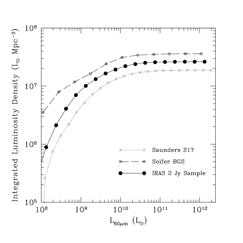
Figure 12: A plot of the cumulative IRAS 60 $\mu$m luminosity density. The filled circles mark the IRAS 2 Jy sample while the filled squares and crosses represent the IRAS BGS sample (Soifer et al. 1987) and the sample “S17” of Saunders et al. (1990).

The derivation of the integrated IRAS 60 $\mu$m luminosity density for the local volume is shown in Figure 12. The derived 60 $\mu$m luminosity density integrated between $L_{60\mu m}=10^{8}L_{\odot}$ and $10^{12}L_{\odot}$ for the IRAS 2 Jy sample is $2.6\pm 0.2\times 10^{7}L_{\odot}$ Mpc^-3. This estimate lies midway between the values derived from the 60 $\mu$m LFs of Soifer et al. (1987) and “S17” of Saunders et al. (1990). These differences arise mainly from the different behaviors of these LFs at low luminosity end (see Fig. 7b and §5.3), and the observed scatter can be interpreted as a measure of uncertainty resulting from the sample selection and clustering of galaxies. In all three cases, the integrated luminosity density reaches the asymptotic peak value near $L_{60\mu m}=10^{11}L_{\odot}$, and the infrared luminous galaxies ($L_{FIR}\geq 10^{11}L_{\odot}$) contribute less than $10\%$ to the FIR luminosity density in the local volume ($z\leq 0.15$).

Using Eq. 3 and assuming a median IRAS 60 $\mu$m to 100 $\mu$m flux ratio of 0.5 (see Figure 10), we estimate a local FIR luminosity density of $(4.8\pm 0.5)\times 10^{7}L_{\odot}$ Mpc^-3. This is midway between the values derived by Soifer et al. ($\sim 9\times 10^{7}L_{\odot}$ Mpc^-3) and Saunders et al. ($4.2\times 10^{7}L_{\odot}$ Mpc^-3). The derived FIR luminosity density can then be used to derive the extinction-free star formation rate (SFR) for the local volume assuming the observed FIR luminosity is proportional to the level of star forming activity.

A wide range of conversion relations between SFR and $L_{FIR}$ are found in the literature, based on either a starburst model or an observational analysis (e.g., Hunter et al. 1986, Meurer et al. 1997, Kennicutt 1998ab). Using the continuous burst model of 10-100 Myr duration by Leitherer & Heckman (1995) and Salpeter IMF with mass limits of 0.1 and 100 $M_{\odot}$, Kennicutt (1998ab) derives a conversion relation appropriate for starbursts as

$${SFR}~{}(M_{\odot}yr^{-1})=1.7\times 10^{-10}L_{8-1000\mu m}(L_{\odot})$$

with about 30% uncertainty. The ratio between $L_{8-1000\mu m}$ and $L_{FIR}$ ($\equiv L_{40-120\mu m}$) for the 60 IRAS BGS galaxies studied by Sanders et al. (1991) ranges between 1.15-2.0 with a median value of about 1.30. Based on actual measurements at both long and short wavelengths, Meurer et al. (1999) find the ratio is larger than 1.4 while Calzetti et al. (2000) find an average value of 1.75 for the five galaxies they examined in detail. Adopting a conservative ratio of 1.5 and using Eq. 13, we derive the star formation rate of $0.012\pm 0.004$ $M_{\odot}$ yr^-1 Mpc^-3 for the local volume ($z\mathrel{\hbox{\raise 2.15277pt\hbox{$<$}\hbox to0.0pt{\hss\lower 2.15277pt\hbox{$\sim$}}}}0.15$). Since more than 90% of the local FIR luminosity density is contributed by normal, late-type field galaxies rather than by the starburst population, a conversion relation derived for late-type field galaxies may be more appropriate for the IRAS 2 Jy sample. The local star formation density derived using the conversion relation derived for the field galaxies by Buat & Xu (1996) is slightly larger, $0.015\pm 0.005$ $M_{\odot}$ yr^-1 Mpc^-3. Contribution from cold cirrus and smaller optical depth in late type galaxies add some uncertainty to the inference of star-formation rate from FIR luminosity (see Kennicutt 1998a for a detailed discussion).

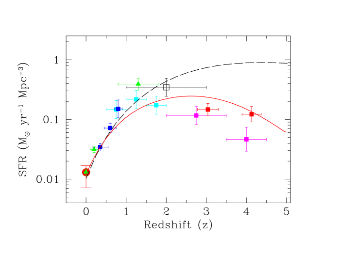
Figure 13: Plot of the cosmic star formation history. The filled triangles and squares represent the SFRs derived from the H$\alpha$ (Gallego et al. 1995, Tresse & Maddox 1998, Yan et al. 1999) and UV continuum (Lilly et al. 1996, Madau et al. 1996, Connolly et al. 1997, Steidel et al. 1999) luminosity density, respectively. All UV density derived values are scaled up by a factor of three to correct for extinction (see Steidel et al. 1999). The large empty square represents the SFR estimated for the faint submm population at $z=1\sim 3$ (Barger et al. 1999). The large filled circle represents the local star formation density derived from the integrated FIR luminosity density, which agrees very well with the SFR derived from H$\alpha$ measurement by Gallego et al. (1995). Two representative models of the star formation evolution by Blain et al. (1999; dashed line) and by Tan et al. (1999; solid line) are also shown after a re-normalization to the new estimate of the current star formation rate.

The two different methods produce a consistent estimate for the local star formation density. In comparison, the the local SFR derived from the H$\alpha$ luminosity density measured by Gallego et al. (1995) using the conversion relation given by Kennicutt (1998a) is $0.014\pm 0.007~{}M_{\odot}$ yr^-1 Mpc^-3. An important consequence is that the local SFR derived from the FIR luminosity density provides an independent estimate for $z=0$ and lends a further support for the $z=0$ normalization for the cosmic star-formation history models such as those by Blain et al. (1999; dashed line) and by Tan et al. (1999; solid line) as well as support for the larger extinction correction for all UV derived values as proposed by Steidel et al. (1999) and others (see Figure 13).

The SFR derived from the FIR luminosity density may be an overestimate if the observed FIR includes a significant contribution from dust heated by an AGN or by interstellar radiation field. The frequency of the radio-excess objects in our sample is only about 1%, independent of luminosity. And the overall frequency of AGNs (including radio-quiet) may be as high as 10% if only one out of ten AGNs produces significant radio emission. Some AGN contribution to the total FIR luminosity density is undoubtedly present, but it is nevertheless not likely to be dominant (see §6.1 & §6.2). The contribution from the dust heated by interstellar radiation field has been suggested previously to account for up to 50 to 70% of the FIR luminosity (see Lonsdale-Persson & Helou 1987, Sauvage & Thuan 1992, Xu & Helou 1996). This claim does not seem entirely consistent with our finding that an overwhelming majority of both the field and starburst galaxies obey the same linear radio-FIR relation (see §3 and §6.2). A possible explanation may be that the cirrus is heated by non-ionizing UV photons from relatively massive stars, so that even the cirrus tracks the population of stars producing the radio emission (Xu 1990).

6.5 1.4 GHz Radio Luminosity and Star Formation Rate

The excellent linear correlation seen between the FIR and radio luminosity among the IRAS 2 Jy sample offers a possibility of deriving the star formation rate directly from the measured radio luminosity. Because of the significant scatter in the radio-FIR relation and possible non-linear effects discussed in §3, determining the star formation rate for any particular galaxy using its radio luminosity alone may be risky. The effect of the scatter is substantially reduced, however, when the radio LF is integrated over luminosity in deriving the radio luminosity density. Further, the star formation density for a given volume can be determined with a greater accuracy if the integration is limited over the range of radio luminosity where the linear radio-FIR relation is secure.

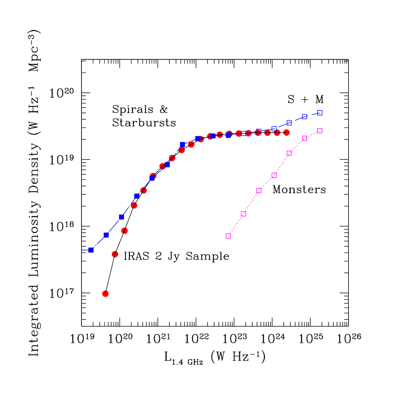
Figure 14: A comparison of the cumulative luminosity density for the 1.4 GHz radio luminosity functions for the IRAS 2 Jy sample with those of the “starbursts & spirals” and “monsters” in the UGC sample studied by Condon (1989). While radio AGNs with lower luminosity are present, they do not contribute significantly to the integrated radio luminosity density below $L_{1.4GHz}\approx 10^{24}$ W Hz^-1.

Deriving the star-formation density from the radio continuum luminosity density for the general galaxy population also has to account for the possible contribution from radio AGNs. As shown in Figure 14, the 1.4 GHz radio LF is dominated by the normal late type galaxies for $L_{1.4GHz}\leq 10^{23}$ W Hz^-1 while the contribution by the “monsters” becomes significant only at $L_{1.4GHz}\geq 10^{24}$ W Hz^-1. This bimodality is also clearly seen in the histogram of 1.4 GHz radio luminosity distribution for Condon’s UGC sample shown in Figure 15. Since the net AGN contribution is small and quantitatively well understood for $L_{1.4GHz}\leq 10^{24}$ W Hz^-1, the star formation density for the local volume can be derived with some confidence from the radio luminosity density integrated up to this luminosity cutoff.

The integrated 1.4 GHz luminosity density derived from the IRAS 2 Jy sample for $L_{1.4GHz}\leq 10^{24}$ W Hz^-1 is $2.6\times 10^{19}$ W Hz^-1 Mpc^-1 (see Figure 14). The empirical conversion relation that links this 1.4 GHz luminosity density to the local star formation density of $0.015\pm 0.005~{}M_{\odot}$ yr^-1 is then

$${SFR}~{}(M_{\odot}yr^{-1})=5.9\pm 1.8\times 10^{-22}L_{1.4GHz}(W~{}Hz^{-1}).$$

As discussed in §6.4, the main uncertainty in this relation comes from the estimate of the local star formation density. If the radio LF at a given epoch can be derived with sufficient accuracy, then the contribution by star forming galaxies and radio AGNs can be distinguished and the star formation density for the epoch can be derived using Eq. 14. Whether the dividing line between the starburst and AGN population near $L_{1.4GHz}\sim 10^{23.5}$ W Hz^-1 is constant or evolved over time is unknown at the moment, and it needs to be investigated by future studies. Ultimately, the cosmic star formation history free of any extinction effects may be derived using the radio emission from star forming galaxies and by tracking the evolution in their radio luminosity function.

7 Conclusions

By cross-correlating the IRAS Redshift Survey catalog and the NRAO VLA Sky Survey database, we have assembled a flux-limited complete sample of 1809 IRAS detected galaxies. This IRAS 2 Jy sample is 6 times larger in size and 5 times deeper in redshift coverage ($z\leq 0.15$) than previous studies of radio and infrared properties of galaxies. In addition to obtaining the accurate positions of these IRAS sources, we have examined the well known radio-FIR correlation in detail. The principal conclusions from the analysis of the data are the following:

1. The radio-FIR correlation for the FIR-selected galaxy sample is well described by a linear relation, and over 98% of the sample galaxies follow this linear radio-FIR correlation. The scatter in the linear relation is about 0.26 in dex, dominated by small systematic deviations involving a small number of galaxies at high and low luminosity ends.

2. A total of 23 “radio-excess” objects (radio AGNs) are found in our sample including three “radio-loud” objects PKS 1345+12, 3C 273, and NGC 1275. The frequency of radio-excess objects in our IRAS 2 Jy sample is 23/1809 = 1.3%, and radio-excess objects are rare among the FIR-selected sample of normal and starburst galaxies. There are only 3 radio-excess objects among the 161 FIR-luminous ($L_{60\mu m}\geq 10^{11.3}L_{\odot}$) galaxies in the sample (3/161 = 1.9%). Therefore the frequency of radio AGNs appears to be independent of FIR luminosity.

3. The derived 1.4 GHz radio luminosity function and 60 $\mu$m luminosity function for the IRAS 2 Jy sample are both reasonably modeled as linear sums of two Schechter functions, one representing late type field galaxies and the second representing a starburst population. The presence of the second, high luminosity component in these LFs is a predictable outcome of the elevated M/L associated with the starburst population, and the Press-Schechter formulation of the structure formation can now be naturally extended to the interpretation of the radio and infrared LFs as well.

4. The radio-excess objects in our sample show evidence for the same highly enhanced radiation field as the infrared luminous galaxies in the infrared color-color diagrams. A systematic segregation of field galaxies, starburst galaxies, and radio AGNs is found in the mid-IR versus far-IR color-color diagram (Fig. 10), where the radio AGNs show the largest observed $S_{25\mu m}/S_{60\mu m}$ ratios. The total fraction of radio-excess objects among the galaxies with mid-IR enhancement is only about 10% (2/20) – similar to the frequency of radio-loud objects among the QSOs. The absence of mid-IR enhancement and radio-excess among the large majority of the IR luminous galaxies suggests that star formation is the dominant energy source in most cases.

5. A small number of infrared-excess objects are also identified by their departure from the radio-FIR relation (9 objects with $q\geq 3$). Both dust-enshrouded AGNs and compact starbursts can explain their observed properties, and distinguishing the two may be difficult. The observed spatial extents of 50-100 pc favors the starburst explanation. In either case, this phase must be brief, perhaps lasting only a few percent of the IR luminous phase since these infrared-excess objects are extremely rare.

6. The integrated 60 $\mu$m luminosity density between $L_{60\mu m}=10^{8}L_{\odot}$ and $10^{12}L_{\odot}$ is $2.6\pm 0.2\times 10^{7}L_{\odot}$ Mpc^-3. The FIR-luminous galaxies ($L_{FIR}\geq 10^{11}L_{\odot}$) contribute less than 10% of the total. The derived local FIR luminosity density is $(4.8\pm 0.5)\times 10^{7}L_{\odot}$ Mpc^-3. The inferred extinction-free star-formation density for the local volume is $0.015\pm 0.005~{}M_{\odot}$ yr^-1 Mpc^-3.

7. The observed linear correlation between the FIR and radio luminosities in the IRAS 2 Jy sample offers a potentially useful method of deriving the star-formation rate using the measured radio luminosity density. A good separation found between star-forming galaxies and AGNs in the derived radio LF offers a promising possibility of tracing the evolution of the two populations separately by deriving their radio LFs at different epochs.

By examining the radio properties of a large sample of infrared selected galaxies, we have obtained a much better understanding of the extent of the radio-FIR correlation. We have also obtained a good quantitative understanding of the frequency and energetic importance of active galactic nuclei among the infrared selected galaxies and outlined the practical limits on using the radio continuum as a direct probe of star forming activity. This study can now serve as the basis for conducting deep radio, IR/submm, and optical surveys aimed at mapping the extinction-free cosmic-star formation history and the evolution of radio AGNs.

Figure 1: Equal area sky projection of the IRAS 2 Jy Sample. Large gap to the right and left of the center trace the Galactic Plane, and a narrow empty strip near the center is the well known gap in the IRAS survey. Otherwise, the sky coverage is fairly uniform.

Figure 2: Plot of 1.4 GHz radio luminosity versus redshift for the IRAS 2 Jy sample. The lower bound is defined by the 2 Jy flux limit of the IRAS 60 $\mu$m band. The upper bound is dictated by the radio luminosity function. The three galaxies with $L_{1.4GHz}\geq 10^{25}$ W Hz^-1 are identified as “radio-loud” objects.

Figure 4: A histogram of the offsets in arcsec between the IRAS PSC and the NVSS catalog positions. The distribution is not Gaussian because the IRAS position error ellipse is typically highly elongated. The position offset is less than 10″ in over 2/3 of the cases, which is consistent with the expectation from the IRAS position uncertainty.

Figure 15: Histogram of 1.4 GHz radio luminosity distribution for the UGC galaxies studied by Condon (1989). The “starbursts” and “monsters” show a relatively clean bimodal separation with a dividing line near $L_{1.4GHz}\approx 10^{23}$ W Hz^-1.

Table 1: Infrared Luminous Galaxies with log $L_{FIR}\geq 11.3L_{\odot}$

Name	$<cz>$	$m$	log $L_{1.4GHz}$	log $L_{60\mu m}$	q	notes
	km/s	mag	(W Hz-1)	$(L_{\odot})$
IRAS 00057$+$4021	13516	16.8	22.47	11.19	2.872
IRAS 00091$-$0738	35509	18.4	23.13	11.79	2.807	jet-like extension to south
IRAS 00188$-$0856	38550	18.4	23.74	11.88	2.315	interacting
IRAS 00234$-$0312	20219	17.0	23.17	11.40	2.409	VV 837, pair
IRAS 00262$+$4251	29129	16.0	23.72	11.66	2.079	LINER
IRAS 00267$+$3016	15119	14.8	23.24	11.28	2.230	MRK 551, blue compact
IRAS 00308$-$2238	18381	17.0	23.06	11.12	2.325
IRAS 00335$-$2732	20771	17.5	23.02	11.54	2.633	starburst
IRAS 00456$-$2904	33060	17.5	23.71	11.70	2.185	interacting, starburst
IRAS 00537$+$1337	24673	16.5	23.37	11.35	2.206
IRAS 01003$-$2238	35286	18.9	23.57	11.70	2.258	HII/WR, Sy2
IRAS 01053$-$1746	6016	14.3	23.29	11.19	2.084	IC1623, pair, HII
IRAS 01106$+$7322	13217	–	22.98	11.16	2.503	Spiral
IRAS 01160$-$0029	14274	15.1	23.01	11.11	2.306	galaxy-pair
IRAS 01173$+$1405	9362	14.9	22.97	11.25	2.416	HII
IRAS 01249$-$0848	14592	15.5	23.23	11.12	2.142	MRK 995
IRAS 01257$+$5015	15522	–	23.09	11.02	2.220	Spiral
IRAS 01264$+$3302	24145	–	23.06	11.36	2.489
IRAS 01364$-$1042	14250	–	22.84	11.22	2.703	LINER
IRAS 01418$+$1651	8245	16.3	22.77	11.22	2.599	pair, HII+LINER
IRAS 01484$+$2220	9705	13.7	23.18	11.12	2.185	NGC 695, pec
IRAS 01572$+$0009	48869	15.2	24.14	12.00	2.012	Sy1
IRAS 02153$+$2636	15016	–	23.04	11.05	2.268
IRAS 02203$+$3158	10142	14.9	23.06	11.09	2.286	MRK 1034, pair of Sy1
IRAS 02290$+$2533	15557	–	23.25	11.06	2.080
IRAS 02378$+$3829	15052	15.7	22.94	11.11	2.369	pair
IRAS 02483$+$4302	15571	–	23.02	11.29	2.502	QSO-galaxy pair
IRAS 02597$+$4455	16087	–	22.94	11.18	2.384	Spiral
IRAS 03119$+$1448	23006	17.3	22.90	11.33	2.597
IRAS 03158$+$4227	40288	17.7	23.68	12.11	2.587
IRAS 03503$-$0328	21730	–	23.09	11.44	2.520
IRAS 03521$+$0028	45622	18.0	23.48	11.99	2.720	LINER
IRAS 03593$-$3149	21462	–	22.99	11.29	2.497
IRAS 04154$+$1755	16659	–	23.61	11.31	1.897	one-sided jet, Sy2
IRAS 04232$+$1436	23972	–	23.56	11.55	2.173	LINER
IRAS 05083$+$7936	16288	15.8	23.38	11.42	2.280	patchy, compact
IRAS 05189$-$2524	12760	15.5	23.01	11.59	2.718	Sy2, pec
IRAS 05246$+$0103	29037	17.0	23.48	11.59	2.232	GPS
IRAS 06076$-$2139	11226	–	22.77	11.16	2.583
IRAS 06102$-$2949	18297	–	23.44	11.43	2.214	triplet in cluster
IRAS 06206$-$3646	32390	–	23.87	11.62	1.919
IRAS 07045$+$4705	19636	–	23.27	11.23	2.145
IRAS 08030$+$5243	25006	17.0	23.33	11.53	2.398
IRAS 08071$+$0509	15650	–	23.28	11.32	2.244	radio jet, HII
IRAS 08323$+$3003	17885	18.0	22.74	11.26	2.693
IRAS 08340$+$1550	23414	–	23.05	11.31	2.459
IRAS 08344$+$5105	29028	–	23.20	11.49	2.478
IRAS 08507$+$3520	16748	15.0	23.38	11.03	1.925	UGC 4653, triple
IRAS 08572$+$3915	17480	–	22.50	11.61	3.218	LINER, Sy2
IRAS 08573$-$0424	18425	17.0	22.94	11.19	2.441
IRAS 08579$+$3447	19645	16.0	23.31	11.29	2.210	Spiral
IRAS 09014$+$0139	16081	17.2	23.06	11.14	2.298
IRAS 09018$+$1447	14847	–	23.69	11.25	1.788	Mrk 1224, quadruple
IRAS 09061$-$1248	22073	15.8	23.30	11.51	2.417
IRAS 09111$-$1007	16438	16.1	23.39	11.56	2.369	radio double, interacting
IRAS 09126$+$4432	11773	14.9	23.04	11.17	2.364	UGC 4881, pair, HII
IRAS 09192$+$2124	23258	–	23.06	11.42	2.516
IRAS 09320$+$6134	11762	15.5	23.70	11.48	2.007	UGC 5101, merger
IRAS 09432$+$1910	16048	–	22.96	11.24	2.452
IRAS 09433$-$1531	15808	16.2	23.17	11.31	2.296
IRAS 09583$+$4714	25717	16.3	23.72	11.52	1.959	Sy1+Sy2
IRAS 10035$+$4852	19421	–	23.36	11.51	2.340	pair
IRAS 10039$-$3338	10223	15.0	22.75	11.28	2.667	IC 2545, pair
IRAS 10173$+$0828	14390	17.5	22.69	11.36	2.808	megamaser
IRAS 10190$+$1322	22987	17.5	23.31	11.50	2.413
IRAS 10311$+$3507	21274	15.0	23.58	11.34	2.007	compact
IRAS 10378$+$1109	40843	17.0	23.51	11.82	2.444
IRAS 10495$+$4424	27616	17.0	23.56	11.66	2.331
IRAS 10502$-$1843	16067	–	23.01	11.29	2.470	Sy2
IRAS 10565$+$2448	12926	16.0	23.31	11.56	2.427	HII, interacting
IRAS 11010$+$4107	10350	–	22.93	11.08	2.379	Arp 148, ring galaxy
IRAS 11011$+$4345	14851	–	23.52	11.22	1.904	pair
IRAS 11069$+$2711	21080	17.0	23.38	11.23	2.109
IRAS 11095$-$0238	31796	17.4	23.75	11.77	2.154	merger
IRAS 11257$+$5850	3101	12.4	23.14	11.32	2.327	NGC 3690, merger
IRAS 11273$-$0607	15687	14.9	23.02	11.07	2.283
IRAS 11379$+$5338	27648	–	23.46	11.46	2.202
IRAS 11506$+$1331	38206	17.1	23.64	11.81	2.355
IRAS 11529$+$8030	13070	16.8	23.05	11.09	2.269	UGC 6896, quartet
IRAS 11554$+$1048	19364	–	22.74	11.22	2.666
IRAS 11598$-$0112	45177	17.9	23.82	11.95	2.294	X-ray source?
IRAS 12071$-$0444	38480	17.8	23.42	11.84	2.551	Sy2
IRAS 12112$+$0305	21703	16.9	23.38	11.85	2.645
IRAS 12120$+$6838	18216	15.4	23.21	11.25	2.305
IRAS 12173$-$3541	17007	–	24.24	11.07	1.081	interacting pair
IRAS 12185$+$1154	20716	17.1	23.36	11.34	2.196	galaxy-pair
IRAS 12265$+$0219	47469	13.1	27.42	11.95	$-$1.277	3c273, blazar
IRAS 12540$+$5708	12518	14.1	24.02	11.98	2.099	MRK 231, Sy1
IRAS 13111$+$4348	17290	–	23.20	11.21	2.241
IRAS 13136$+$6223	9313	15.1	23.03	11.25	2.384	UGC 8335, pair, HII
IRAS 13183$+$3423	6894	14.8	23.03	11.11	2.302	IC 883, merger, LINER
IRAS 13225$-$2614	18468	16.2	22.77	11.15	2.556	merger? starburst
IRAS 13333$-$1700	14990	–	22.88	11.18	2.460	starburst
IRAS 13336$-$0046	17859	–	23.19	11.16	2.194	UGC 8584, triple
IRAS 13428$+$5608	11180	15.0	23.59	11.73	2.282	MRK 273, Sy2, LINER
IRAS 13438$-$0037	23058	–	23.24	11.32	2.300
IRAS 13451$+$1232	36341	17.0	26.18	11.68	$-$0.341	Sy2, merger
IRAS 13454$-$2956	22728	18.6	23.11	11.34	2.450	LINER
IRAS 14104$-$1350	22040	16.1	23.38	11.37	2.195
IRAS 14147$-$2248	23850	–	23.15	11.41	2.433
IRAS 14158$+$2741	20902	16.0	23.37	11.26	2.118
IRAS 14290$-$2729	17225	–	22.87	11.09	2.451
IRAS 14348$-$1447	24677	16.6	23.67	11.87	2.368	LINER, merger
IRAS 14351$-$1954	26886	–	23.36	11.48	2.325
IRAS 14378$-$3651	20277	16.3	23.49	11.68	2.354	E?
IRAS 14394$+$5332	31450	17.2	23.96	11.57	1.776
IRAS 14547$+$2448	10166	14.6	23.32	11.08	2.056	UGC 9618, galaxy pair
IRAS 15018$+$2417	20685	16.5	23.26	11.36	2.299
IRAS 15163$+$4255	12049	14.9	23.20	11.39	2.353	MRK 848, HII+LINER
IRAS 15179$+$3956	14172	16.0	22.32	11.17	2.984	merger
IRAS 15233$+$0533	16227	–	22.86	11.24	2.535
IRAS 15238$-$3058	14318	–	23.28	11.06	2.095
IRAS 15245$+$1019	22687	15.8	23.27	11.52	2.452
IRAS 15250$+$3609	16602	16.0	22.95	11.58	2.752	ring galaxy, LINER
IRAS 15320$-$2601	20549	–	22.98	11.40	2.585
IRAS 15327$+$2340	5534	14.4	23.33	11.77	2.607	Arp 220, Sy2, LINER
IRAS 15462$-$0450	30150	16.4	23.41	11.72	2.459	disturbed pair, Sy1
IRAS 15473$-$0520	16994	–	22.51	11.17	2.801
IRAS 16090$-$0139	40029	16.6	23.87	12.03	2.344	LINER
IRAS 16133$+$2107	27206	–	23.18	11.48	2.482
IRAS 16161$+$4015	23288	–	23.17	11.36	2.405
IRAS 16305$+$4823	26329	–	23.04	11.40	2.523
IRAS 16429$+$1947	24735	–	23.25	11.43	2.391
IRAS 16474$+$3430	33418	16.5	23.44	11.66	2.403
IRAS 16487$+$5447	31293	16.5	23.61	11.70	2.264
IRAS 16504$+$0228	7298	14.7	23.69	11.33	1.822	NGC 6240, LINER, Sy2
IRAS 17028$+$5817	31779	–	23.56	11.66	2.318
IRAS 17132$+$5313	15270	–	23.18	11.42	2.426	merging pair
IRAS 17208$-$0014	12836	15.1	23.46	12.00	2.703	HII
IRAS 17409$+$1554	22042	–	23.05	11.25	2.385
IRAS 17465$-$0339	22538	–	23.30	11.39	2.245
IRAS 17487$+$5637	19687	16.9	22.97	11.27	2.546
IRAS 17501$+$6825	15357	15.2	23.12	11.06	2.194
IRAS 17517$+$6422	26151	–	23.21	11.40	2.396
IRAS 17574$+$0629	32860	16.5	23.53	11.63	2.263	E
IRAS 18214$-$3931	34005	–	23.11	11.70	2.755
IRAS 18293$-$3413	5449	–	23.16	11.30	2.344	HII, pair
IRAS 18368$+$3549	34825	16.3	23.74	11.69	2.180
IRAS 18443$+$7433	40395	17.3	23.60	11.80	2.358
IRAS 18470$+$3233	23626	16.0	23.19	11.63	2.569
IRAS 18544$-$3718	22012	–	22.79	11.40	2.806
IRAS 19096$+$4502	18980	–	23.22	11.25	2.262	pair, HII+HII
IRAS 19115$-$2124	14608	–	23.45	11.38	2.156	interacting pair
IRAS 19297$-$0406	25674	16.0	23.62	11.94	2.488	merger, HII
IRAS 20010$-$2352	15249	16.9	22.89	11.19	2.488	Sy2
IRAS 20046$-$0623	25362	16.3	23.32	11.59	2.444	interacting pair
IRAS 20087$-$0308	31600	16.1	23.11	11.92	3.009	merger
IRAS 20210$+$1121	16905	15.8	23.52	11.29	1.873	interacting, Sy2
IRAS 20414$-$1651	26107	17.1	23.55	11.76	2.378
IRAS 20550$+$1656	10900	15.2	23.05	11.44	2.523	IIZw096, interacting
IRAS 20567$-$1109	15221	–	23.26	11.16	2.068
IRAS 21316$-$1729	17050	–	22.59	11.23	2.812
IRAS 21396$+$3623	29034	16.5	23.41	11.51	2.328
IRAS 21442$+$0007	22187	–	23.10	11.27	2.413
IRAS 21504$-$0628	23263	15.6	23.28	11.56	2.407
IRAS 22491$-$1808	23312	16.2	22.84	11.74	3.025	merger, HII
IRAS 23050$+$0359	14205	–	22.85	11.13	2.474
IRAS 23204$+$0601	16779	16.0	23.08	11.33	2.407	blue E
IRAS 23327$+$2913	31981	–	23.27	11.58	2.493
IRAS 23365$+$3604	19338	16.3	23.36	11.71	2.514	disturbed, LINER
IRAS 23410$+$0228	27335	17.8	23.02	11.50	2.608	disburbed, X-ray source?

Table 2: Radio-excess Objects

Name	$<cz>$	$m$	log $L_{1.4GHz}$	log $L_{60\mu m}$	q	notes
	km/s	mag	(W Hz-1)	$(L_{\odot})$
IRAS 03164$+$4119	5486	12.4	25.13	10.57	$-$0.463	3C84, NGC1275
IRAS 03208$-$3723	1780	9.9	22.24	9.26	1.511	NGC 1316, Fornax A
IRAS 05497$-$0728	2334	14.0	22.54	9.65	1.301	NGC 2110, Sy 2
IRAS 05511$+$4625	6009	13.9	23.28	10.32	1.254	UGC3374, Sy 1
IRAS 06097$+$7103	4050	13.8	23.59	10.06	0.618	UGC3426, Sy 2
IRAS 06488$+$2731	12270	14.9	23.71	10.83	1.253	Sy 2
IRAS 07224$+$3003	5730	–	23.01	10.25	1.434	UGC3841, FR-I RG
IRAS 08400$+$5023	3226	12.4	22.41	9.57	1.549	NGC2639, Sy 2
IRAS 10459$-$2453	3730	14.8	22.39	9.77	1.616	NGC3393, Sy 2
IRAS 11220$+$3902	2080	12.0	22.02	9.19	1.535	NGC3665, radio jet
IRAS 12080$+$3941	995	11.5	22.19	9.81	1.388	NGC4151, Sy 1.5
IRAS 12173$-$3541	17007	–	24.24	11.07	1.083	pair
IRAS 12265$+$0219	47469	13.1	27.42	11.95	$-$1.277	3C273, QSO
IRAS 13184$+$0914	9565	15.1	23.30	10.54	1.520	NGC5100, pair
IRAS 13197$-$1627	5152	14.6	23.19	10.43	1.402	Sy 2
IRAS 13443$+$1439	6435	15.5	23.23	10.35	1.379	Mrk 796, Sy 2
IRAS 13451$+$1232	36341	17.0	26.18	11.68	$-$0.341	4C12.50, Sy 2
IRAS 13536$+$1836	14895	14.8	24.26	10.95	0.844	Mrk 463, Sy 1
IRAS 14106$-$0258	1753	13.6	22.35	9.69	1.506	NGC5506, Sy 2
IRAS 15060$+$3434	13500	–	23.72	10.93	1.475	VV 59, pair
IRAS 21497$-$0824	10330	–	23.61	10.79	1.363
IRAS 22045$+$0959	7800	15.1	23.17	10.51	1.575	NGC7212, Sy 2
IRAS 23254$+$0830	8698	13.6	23.55	10.88	1.530	NGC7674, Sy 2

Table 3: Infrared-excess Objects

Name	$<cz>$	$m$	log $L_{1.4GHz}$	log $L_{60\mu m}$	q	notes
	km/s	mag	(W Hz-1)	$(L_{\odot})$
IRAS 02244$+$4146	5606	15.0	21.54	10.35	3.075
IRAS 02330$-$0934	1509	11.0	20.36	9.12	3.085	NGC988
IRAS 04332$+$0209	3580	15.6	21.09	9.96	3.070	UGC3097
IRAS 04489$+$1029	8416	–	21.87	10.47	3.086
IRAS 08572$+$3915	17480	14.9	22.50	11.61	3.218	LINER, Sy2
IRAS 12243$-$0036	2179	14.2	21.62	10.57	3.075	NGC4418
IRAS 19420$-$1450	-57	9.4	18.45	7.79	3.184	NGC6822
IRAS 20087$-$0308	31600	16.1	23.11	11.92	3.009	merger
IRAS 22491$-$1808	23312	16.2	22.84	11.74	3.025	merger, HII

Table 4: IRAS $60\mu m$ Luminosity Distribution and Luminosity Function

log $L_{60\mu m}$	N	log $\rho_{60\mu m}$	$V/V_{m}$
$(L_{\odot})$		(Mpc-3 mag-1)
7.875	2	$-2.44^{+0.23}_{-0.53}$	$0.205\pm 0.320$
8.125	6	$-2.34^{+0.15}_{-0.23}$	$0.307\pm 0.226$
8.375	16	$-2.29^{+0.10}_{-0.12}$	$0.449\pm 0.168$
8.625	34	$-2.34^{+0.07}_{-0.09}$	$0.464\pm 0.117$
8.875	68	$-2.41^{+0.05}_{-0.06}$	$0.491\pm 0.085$
9.125	95	$-2.64^{+0.04}_{-0.05}$	$0.490\pm 0.072$
9.375	128	$-2.89^{+0.04}_{-0.04}$	$0.411\pm 0.057$
9.625	182	$-3.11^{+0.03}_{-0.03}$	$0.447\pm 0.050$
9.875	203	$-3.44^{+0.03}_{-0.03}$	$0.495\pm 0.049$
10.125	277	$-3.68^{+0.03}_{-0.03}$	$0.506\pm 0.043$
10.375	242	$-4.11^{+0.03}_{-0.03}$	$0.507\pm 0.046$
10.625	210	$-4.55^{+0.03}_{-0.03}$	$0.547\pm 0.051$
10.875	138	$-5.11^{+0.04}_{-0.04}$	$0.480\pm 0.059$
11.125	83	$-5.70^{+0.05}_{-0.05}$	$0.467\pm 0.075$
11.375	57	$-6.24^{+0.05}_{-0.06}$	$0.534\pm 0.097$
11.625	38	$-6.79^{+0.07}_{-0.08}$	$0.525\pm 0.118$
11.875	17	$-7.51^{+0.09}_{-0.12}$	$0.492\pm 0.170$
12.125	4	$-8.52^{+0.18}_{-0.30}$	$0.387\pm 0.311$

Table 5: Schechter Parameters for the IRAS 60 $\mu$m Luminosity Distribution and Function

Functions	$L^{*}$	$\alpha$	$\rho^{*}V^{*}$	$\chi^{2}$
and Fits	($10^{10}L_{\odot}$)		or $\rho^{*}$
$n(L)-$low $L$	$2.24\pm 0.41$	$-0.805\pm 0.058$	$509\pm 160$	$6.2$
$n(L)-$high $L$	$21.46\pm 1.82$	$-0.805\pm 0.058$	$143\pm 8$	$4.1$
$n(L)-$single fit	$15.38\pm 0.74$	$-1.221\pm 0.019$	$309\pm 35$	$232$
$\rho(L)-$low $L$	$2.33\pm 0.48$	$-0.821\pm 0.072$	$(2.23\pm 0.29)\times 10^{-4}$	$4.4$
$\rho(L)-$high $L$	$21.69\pm 1.85$	$-0.821\pm 0.072$	$(2.21\pm 0.13)\times 10^{-6}$	$4.1$
$\rho(L)-$single fit	$15.38\pm 0.73$	$-1.220\pm 0.019$	$(0.81\pm 0.07)\times 10^{-5}$	$234$

Table 6: 1.4 GHz Radio Luminosity Distribution and Luminosity Function

log $L_{1.4GHz}$	N	log $\rho_{1.4GHz}$	$V/V_{m}$
(W Hz-1)		(Mpc-3 mag-1)
19.625	3	$-2.64^{+0.20}_{-0.37}$	$0.211\pm 0.265$
19.875	8	$-2.43^{+0.19}_{-0.34}$	$0.284\pm 0.188$
20.125	10	$-2.46^{+0.14}_{-0.21}$	$0.427\pm 0.207$
20.375	35	$-2.30^{+0.08}_{-0.10}$	$0.444\pm 0.113$
20.625	49	$-2.49^{+0.07}_{-0.08}$	$0.474\pm 0.098$
20.875	66	$-2.54^{+0.07}_{-0.08}$	$0.428\pm 0.081$
21.125	94	$-2.78^{+0.05}_{-0.06}$	$0.489\pm 0.072$
21.375	128	$-2.96^{+0.04}_{-0.05}$	$0.406\pm 0.056$
21.625	186	$-3.11^{+0.04}_{-0.04}$	$0.486\pm 0.051$
21.875	228	$-3.41^{+0.04}_{-0.04}$	$0.495\pm 0.047$
22.125	294	$-3.60^{+0.05}_{-0.06}$	$0.512\pm 0.042$
22.375	241	$-4.06^{+0.04}_{-0.05}$	$0.505\pm 0.046$
22.625	181	$-4.52^{+0.06}_{-0.08}$	$0.535\pm 0.054$
22.875	115	$-5.10^{+0.06}_{-0.07}$	$0.465\pm 0.064$
23.125	71	$-5.56^{+0.09}_{-0.12}$	$0.534\pm 0.087$
23.375	46	$-6.00^{+0.14}_{-0.20}$	$0.494\pm 0.104$
23.625	32	$-5.95^{+0.22}_{-0.49}$	$0.501\pm 0.125$
23.875	4	$-7.96^{+0.20}_{-0.37}$	$0.753\pm 0.434$
24.125	3	$-7.58^{+0.28}_{-1.03}$	$0.561\pm 0.433$

Table 7: Schechter Parameters for the 1.4 GHz Radio Luminosity Function

Functions	$L^{*}$	$\alpha$	$\rho^{*}$	$\chi^{2}$
	(1022 W Hz-1)
$\rho(L)-$low $L$	$2.11\pm 0.28$	$-0.633\pm 0.051$	$(3.17\pm 0.17)\times 10^{-4}$	$5.9$
$\rho(L)-$High $L$	$14.43\pm 1.65$	$-0.633\pm 0.051$	$(0.83\pm 0.08)\times 10^{-5}$	$7.5$
$\rho(L)-$single fit	$10.76\pm 0.84$	$-0.988\pm 0.028$	$(2.43\pm 0.08)\times 10^{-5}$	$112$

References

- Alloin et al. (1992) Alloin, D., Barvainis, R., Gordon, M. A., & Antonucci, R. R. J. 1992, A&A, 265, 429
- Auriemma et al. (1977) Auriemma, C., Perola, G. C., Ekers, R., Fanti, R., Lari, C., Jaffe, W. J., & Ulrich, M. H. 1977, A&A, 57, 41
- Bahcall et al. (1997) Bahcall, J. N., Kirhakos, S., Saxe, D. H., & Schneider, D. P. 1997, ApJ, 479, 642
- Barger et al. (1999) Barger, A. J., Cowie, L. L., Smail, I., Ivison, R. J., Blain, A. W., & Kneib, J.-P. 1999, AJ, 117, 2656
- Beichman et al. (1986) Beichman, C. A., Soifer, B. T., Helou, G., Chester, T. J., Neugebauer, G., Gillett, F. C., & Low, F. J. 1986, ApJ, 308, L1
- Blain et al. (1999) Blain, A., Smail, I., Ivison, R. J., & Kneib, J.-P. 1999, MNRAS, 302, 632
- Buat & Xu (1996) Buat, V., & Xu, C. 1996, A&A, 306, 61
- Bushouse (1987) Bushouse, H.A. 1987, ApJ, 320, 49
- Calzetti et al. (2000) Calzetti, D., Armus, L., Bohlin, R. C., Kinney, A. L., Koornneef, J. et al. 2000, ApJ, 533, 682
- Carilli & Yun (1999a) Carilli, C. L., & Yun, M. S. 1999, ApJ, 513, L13
- Chi & Wolfendale (1990) Chi, X., & Wolfendale, A. W. 1990, MNRAS, 245, 101
- Condon (1984) Condon, J. J. 1984, ApJ, 287, 461
- Condon (1987) Condon, J. J. 1987, ApJS, 65, 485
- Condon (1989) Condon, J. J. 1989, ApJ, 338, 13
- Condon (1992) Condon, J. J. 1992, ARAA, 30, 575
- Condon & Broderick (1986) Condon, J. J., & Broderick, J. J. 1988, AJ, 92, 94
- Condon & Broderick (1988) Condon, J. J., & Broderick, J. J. 1988, AJ, 96, 30
- Condon et al. (1990) Condon, J. J., Helou, G., Sanders, D. B., & Soifer, B. T. 1990, ApJS, 73, 359
- Condon, Anderson, & Helou (1991a) Condon, J. J., Anderson, M. L., & Helou, G. 1991a, ApJ, 376, 95
- Condon et al. (1991b) Condon, J. J., Huang, Z. P., Yin, Q. F., & Thuan, T. X. 1991b, ApJ, 378, 65
- Condon et al. (1998) Condon, J. J., Cotton, W. D., Greison, E. W., Yin, Q. F., Perley, R. A., et al. 1998, AJ, 115, 1693
- Connolly et al. (1997) Connolly, A. J., Szalay, A. S., Dickinson, M., Subbarao, M. U., & Brunner, R. J. 1997, ApJ, 486, L11
- Conway et al. (1993) Conway, R. G., Garrington, S. T., Perley, R. A., & Biretta, J. A. 1993, A&A, 267, 347
- Cotton & Condon (1998) Cotton, W. D., & Condon, J. J. 1998, in Observational Cosmology with the New Radio Surveys, eds. M. N. Bremer et al., (Dordrecht: Kluwer Academic Publishers), p.45
- Cox et al. (1988) Cox, M. J., Eales, S. A. E., Alexander, P., & Fitt, A. J. 1988, MNRAS, 235, 1227
- Crawford et al. (1996) Crawford, T., Marr, J., Partridge, B., & Strauss, M. A. 1996, ApJ, 460, 225
- Cutri et al. (1994) Cutri, R. M., Huchra, J. P., Low, F. J., Brown, R. L., & Vanden Bout, P. A. 1994, ApJ, 424, L65
- de Grijp et al. (1985) de Grijp, M. H. K., Miley, G. K., Lub, J., & de Jong, T. 1985, Nature, 314, 240
- de Jong et al. (1984) de Jong, T., Clegg, P. E., Soifer, B. T., Rowan-Robinson, M., Habing, H. J., et al. 1984, ApJ, 278, L67
- de Jong et al. (1985) de Jong, T., Klein, U., Wielebinski, R., and Wunderlich, E. 1985, A&A, 147, L6
- Désert (1986) Désert, F. X. 1986, in Light on Dark Matter, ed. F. P. Israel (Dordrecht: Reidel), p.213
- Devereux & Eales (1989) Devereux, N. A., & Eales, S. A. 1989, ApJ, 340, 708
- Eales et al. (1999) Eales, S., Lilly, S., Gear, W., Dunne, L., Bond, J. R. et al. 1999, ApJ, 515, 518
- Efstathiou, Ellis, & Peterson (1988) Efstathiou G., Ellis, R. S., & Peterson, B. A. 1988, MNRAS, 232, 431
- Efstathiou et al. (2000) Efstathiou, A., Rowan-Robinson, M., & Siebenmorgen, R. 2000, MNRAS, 313, 734
- Fabian et al. (1981) Fabian, A. C., Hu, E. M., Cowie, L. L., & Grindlay, J. 1981, ApJ, 248, 47
- Evans et al. (1999) Evans, A. S., Kim, D. C., Mazzarella, J. M., Scoville, N. Z., & Sanders, D. B. 1999, ApJ, 521, L107
- Felten (1976) Felten, J. E. 1976, ApJ, 207, 700
- Fisher et al. (1995) Fisher, K. B., Huchra, J. P., Strauss, M. A., Davis, M., Yahil, A., & Schlegel, D. 1995, ApJS, 100, 69
- Fitt, Alexander, & Cox (1988) Fitt, A. J., Alexander, P., & Cox, M. J. 1988, MNRAS, 233, 907
- Gallego et al. (1995) Gallego, J., Zamorano, J., Arag’on-Salamanca, A., & Rego, M. 1995, ApJ, 455, L1
- Gardner et al. (1997) Gardner, J. P., Sharples, R. M., Frenck, C. S., & Carrasco, B. E. 1997, ApJ, 480, L99
- Genzel et al. (1998) Genzel, R., Lutz, D., Sturm, E., Egami, E., Kunze, D. et al. 1998, ApJ, 498, 579
- Gilmore & Shaw (1986) Gilmore, G. F., & Shaw, M. A. 1986, Nature, 321, 750
- Harwit & Pacini (1975) Harwit, M., & Pacini, F. 1975, ApJ, 200, L127
- Helou (1986) Helou, G. 1986, ApJ, 311, L33
- Helou et al. (1985) Helou, G., Soifer, B. T., & Rowan-Robinson, M. 1985, ApJ, 298, L7
- Helou et al. (1988) Helou, G., Khan, I. R., Malek, L., & Boehmer, L. 1988, ApJS, 68, 151
- Ho & Ulvestad (2000) Ho, L. C., & Ulvestad, J. S. 2000, ApJS, in submitted.
- Hooper et al. (1995) Hooper, E. J., Impey, C. D., Foltz, C. B. & Hewett, P. C. 1995, ApJ, 445, 62
- Hughes et al. (1998) Hughes, D. H. et al. 1998, Nature, 394, 241
- Hummel (1981) Hummel, E 1981, A&A, 93, 93
- Hunter et al. (1986) Hunter, D. A., Gillett, F. C., Gallagher III, J. S., Rice, W. L., & Low, F. J. 1986, ApJ, 303, 171
- Hutchings & Neff (1988) Hutchings, J. B., & Neff, S. G. 1988, AJ, 96, 1575
- Inoue et al. (1996) Inoue, M. Y., Kameno, S., Kawabe, R., Inoue, M., Hasegawa, T., & Tanaka, M. 1996, AJ, 111, 1852
- Isobe & Feigelson (1992) Isobe, T., & Feigelson, E. D. 1992, ApJS, 79, 197
- Kellermann et al. (1989) Kellermann, K. I., Sramek, R., Schmidt, M., Shaffer, D. B., Green, R. 1989, AJ, 98, 1195
- Kennicutt (1998a) Kennicutt, Jr. R. C. 1998a, ARAA, 36, 189
- Kennicutt (1998b) Kennicutt, Jr. R. C. 1998b, ApJ, 498, 541
- Kent & Sargent (1979) Kent, S. M., & Sargent, W. L. W. 1979, ApJ, 230, 667
- Klein et al. (1984) Klein, U., Wielebinski, R., & Thuan, T. X. 1984, A&A, 141, 241
- Langston et al. (1990) Langston, G. I., Conner, S. R., Heflin, M. B., Lehar, J., & Burke, B. F. 1990, ApJ, 353, 34
- Lawrence et al. (1986) Lawrence, A., Walker, D., Rowan-Robinson, M., Leech, K. J., & Penston, M. V. 1986, MNRAS, 219, 687
- Leitherer & Heckman (1995) Leitherer, C., & Heckman, T. M. 1995, ApJS, 96, 9
- Lester et al. (1995) Lester, D. F., Zink, E. C., Doppmann, G. W., Gaffney, N. I., Harvey, P. M., et al. 1995, ApJ, 439, 185
- Lilly et al. (1996) Lilly, S., Le Fevre, O., Hammer, F., Crampton, D. 1996, ApJ, 460, L1
- Lisenfeld, Volk, & Xu (1996) Lisenfeld, U., Volk, H. J., & Xu, C. 1996, A&A, 314, 745
- Lonsdale-Persson & Helou (1987) Lonsdale-Persson, C. J., & Helou, G. 1987, ApJ, 314, 513
- Loveday (2000) Loveday, J. 2000, MNRAS, 312, 557
- Madau et al. (1996) Madau, P., Ferguson, H. C., Dickinson, E., Giavalisco, M., Steidel, C. C., & Fruchter, A. 1996, MNRAS, 283, 1388
- Meurer et al. (1997) Meurer, G. R., Heckman, T. M., Lehnert, M. D., Leitherer, C., & Lowenthal, J. 1997, AJ, 114, 54
- Meurer et al. (1999) Meurer, G. R., Heckman, T. M., Calzetti, D. 1999, ApJ, 521, 64
- Miley & Perola (1975) Miley, G. K., & Perola, G. C. 1975, A&A, 45, 223
- Mirabel et al. (1989) Mirabel, I. F., Sanders, D. B., & Kazès, I. 1989, ApJ, 340, L9
- Neugebauer et al. (1984) Neugebauer, G., Habing, H. J., van Duinen, R., Aumann, H. H., Baud, B., et al. 1984, ApJ, 278, L1
- Nilson (1973) Nilson, P. 1973, Uppsala General Catalogue of Galaxies, (Uppsala universitet Acta Universitatis Upsaliensis).
- Oliver et al. (1996) Oliver, S. J., Rowan-Robinson, M., Broadhurst, T. J., McMahon, R. G, Saunders, W. et al.1996, MNRAS, 280, 673
- Pedlar et al. (1990) Pedler, A., Ghataure, H. S., Davies, R. D., Harrison, B. A., Perley, R. A. et al. 1990, MNRAS, 246, 477
- Press & Schechter (1974) Press, W. H., & Schechter, P. 1974, ApJ, 187, 425
- Price & Duric (1992) Price, R., & Duric, N. 1992, ApJ, 401, 81
- Rickard & Harvey (1984) Rickard, L. J., & Harvey, P. M. 1984, AJ, 89, 1520
- Rice et al. (1988) Rice, W, Lonsdale, C. J., Soifer, B. T., Neugebauer, G., Kopan, E. L. et al. 1988, ApJS, 68, 91
- Sandage et al. (1979) Sandage, A., Tammann, G. A., & Yahil, A. 1979, ApJ, 232, 352
- Sanders et al. (1989) Sanders, D. B., Phinney, E. S., Neugebauer, G., Soifer, B. T., & Matthews, K. 1989, ApJ, 347, 29
- Sanders & Mirabel (1996) Sanders, D. B., & Mirabel, I. F. 1996, ARAA, 34, 749
- Saunders et al. (1990) Saunders, W., Rowan-Robinson, M., Lawrence, A., Efstathiou, G., Kaiser, N. et al. 1990, MNRAS, 242, 318
- Sauvage & Thuan (1992) Sauvage, M., & Thuan, T. X. 1992, ApJ, 396, L69
- Schechter (1976) Schechter, P. 1976, ApJ, 203, 297
- Schmidt (1963) Schmidt, M. 1963, Nature, 197, 1040
- Schmidt (1968) Schmidt, M. 1968, ApJ, 151, 393
- Shapiro (1971) Shapiro, S. L. 1971, AJ, 76, 291
- Shaw, Tzioumis, & Pedlar (1992) Shaw, M. A., Tzioumis, A. K., & Pedlar, A. 1992, MNRAS, 256, 6
- Smail, Ivison, & Blain (1997) Smail, I., Ivison, R. J., & Blain, A. W. 1997, ApJ, 490, L5
- Smail et al. (2000) Smail, I., Ivison, R. J., Owen, F. N., Blain, A. W., & Kneib, J.-P. 2000, ApJ, 528, 612
- Smith et al. (1987) Smith, B. J., Kleinmann, S. G., Huchra, J. P., & Low, F. J. 1987, ApJ, 318, 161
- Soifer et al. (1984) Soifer, B. T., Rowan-Robinson, M., Houck, J. R., de Jong, T., Neugebauer et al. 1984, ApJ, 278, L71
- Soifer et al. (1987) Soifer, B. T., Sanders, D. B., Madore, B. F., Neugebauer, G., Danielson, G. E. et al. 1987, ApJ, 320, 238
- Steidel et al. (1999) Steidel, C., Adelberger, K. L., Giavalisco, M., Dickinson, M., & Pettini, M. 1999, ApJ, 519, 1
- Stockton (1980) Stockton, A. 1980, in Objects of High Redshift, (Dordrecht: Reidel), p.89
- Strauss & Huchra (1988) Strauss, M. A., & Huchra, J. 1988, AJ, 95, 1602
- Strauss et al. (1990) Strauss, M. A., Davis, M., Yahil, A., & Huchra, J. P. 1990, ApJ, 361, 49
- Strauss et al. (1992) Strauss, M. A., Huchra, J. P., Yahil, A., Fisher, K. B., & Tonry, J. 1992, ApJS, 83, 29
- Szokoly et al. (1998) Szokoly, G. P., Subbarao, M. U., Connolly, A. J., & Mobasher, B 1998, ApJ, 492, 452
- Tan et al. (1999) Tan, J. C., Silk, J., & Balland, C. 1999, ApJ, 522, 579
- Tresse & Maddox (1998) Tresse, L., & Maddox, S. J. 1998, ApJ, 495, 691.
- Treyer et al. (1998) Treyer, M. A., Ellis, R. S., Milliard, B., Donas, J., & Bridges, T. J. 1998, MNRAS, 300, 303
- Unger et al. (1989) Unger, S. W., Wolstencroft, R. D., Pedlar, A., Savage, A., Clowes, R. G. et al. 1989, MNRAS, 236, 425
- van Breugel et al. (1984) van Breugel, W., Miley, G., & Heckman, T. 1984, AJ, 89, 5
- Veilleux, Sanders, & Kim (1997) Veilleux, S., Sanders, D. B., & Kim, D. C. 1997, ApJ, 484, 92
- Wunderlich & Klein (1988) Wunderlich, E., & Klein, U. 1988, A&AS, 206, 47
- Xu (1990) Xu, C. 1990, ApJ, 365, L47
- Xu & Helou (1996) Xu, C., & Helou, G. 1996, ApJ, 456, 163
- Yahil et al. (1991) Yahil, A., Strauss, M. A., Davis, M., & Huchra, J. P. 1991, ApJ, 372, 380
- Yan et al. (1999) Yan, L., McCarthy, P. J., Freudling, W., Teplitz, H. I., Malumuth, E. M. et al. 1999, ApJ, 519, L47
- Yun & Scoville (1998) Yun, M. S., & Scoville, N. Z. 1998, ApJ, 507, 774
- Yun et al. (2000) Yun, M. S., Carilli, C. L., Kawabe, R., Tutui, Y., Kohno, K., & Ohta, K. 2000, ApJ, 528, 171